The geometrical nature and some properties of the capacitance coefficients based on the Laplace’s equation

Abstract

The fact that the capacitance coefficients for a set of conductors are geometrical factors is derived in most electricity and magnetism textbooks. We present an alternative derivation based on Laplace’s equation that is accessible for an intermediate course on electricity and magnetism. The properties of Laplace’s equation permits to prove many properties of the capacitance matrix. Some examples are given to illustrate the usefulness of such properties.

I Introduction

The fact that the capacitance is a geometrical factor is an important property in courses on electricity and magnetism.Berkeley ; Jack Derivations of this property are usually based on the principle of superpositionBerkeley ; Jack and the Green function formalismUehara ; Lorenzo . Nevertheless, such derivations are not convenient for calculations. Alternative techniques to calculate the capacitance coefficients based on the Green function formalismDonolato and other methodsCui ; Bodegom ; Tong have been developed.

In this paper we give a simple proof of the geometrical nature of the capacitance coefficients based on Laplace’s equation. Our approach permits to demonstrate many properties of the capacitance matrix. The method is illustrated by reproducing some well known results, and applications in complex situations are suggested.

II Capacitance coefficients

We consider a system of $N$ internal conductors and an external conductor that encloses them. The potential on each internal conductor is denoted by $\varphi_{i}$, $i=1,2,\ldots,N$. The surface of the external conductor is denoted by $S_{N+1}$, and its potential is denoted by $\varphi_{N+1}$ (see Fig. 1). One reason to introduce the external conductor is that it provides a closed boundary to ensure the uniqueness of the solutions. In addition, many capacitors contain an enclosing conductor as for the case of spherical concentric shells. As we shall see, the case in which there is no external conductor can be obtained in the appropriate limit.

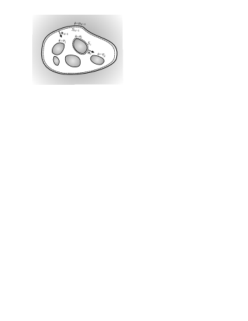
Figure 1: A system consisting of $N$ internal conductors with conductor $N+1$ enclosing them. The normals $\mathbf{n}_{i}$ with $i=1,\ldots,N+1$ point outward with respect to the conductors and inward with respect to the volume $V_{S_{T}}$ (defined by the region in white). The surfaces $S_{i}$ with $i=1,\ldots,N$ are slightly bigger than the ones corresponding to the conductors. In contrast, the surface $S_{N+1}$ is slightly smaller than the surface of the external conductor.

The surface charge density $\sigma$ on an electrostatic conductor is given byBerkeley ; Jack

$$\sigma_{i}=\varepsilon_{0}\mathbf{E}\cdot\mathbf{n}_{i}=-\varepsilon_{0}\nabla\phi\cdot\mathbf{n}_{i}\qquad(i=1,\ldots,N+1),$$ (1)

where $\mathbf{n}_{i}$ is an unit vector normal to the surface $S_{i}$ pointing outward with respect to the conductor (see Fig. 1); $\mathbf{E}$ and $\phi$ denote the electrostatic field and potential respectively. The charge on each conductor is given by

$$Q_{i}=\!\oint_{S_{i}}\sigma_{i}\,dS=-\varepsilon_{0}\!\oint_{S_{i}}\nabla\phi\cdot\mathbf{n}_{i}\,dS.$$ (2)

The surface $S_{i}$ encloses the conductor $i$ and is arbitrarily near and locally parallel to the real surface of the conductor (see Fig. 1).note1 We define the total surface $S_{T}$ as

$$S_{T}=S_{1}+\ldots+S_{N}+S_{N+1}.$$ (3)

The volume $V_{S_{T}}$ defined by the surface $S_{T}$ is the one delimited by the external surface $S_{N+1}$ and the $N$ internal surfaces $S_{i}$. The potential $\phi$ in such a volume must satisfy Laplace’s equation with the boundary conditions

$$\phi(S_{i})=\varphi_{i}\qquad(i=1,\ldots,N+1).$$ (4)

Because of the linearity of Laplace’s equation, the solution for $\phi$ can be parameterized as

$$\phi=\sum_{j=1}^{N+1}\varphi_{j}f_{j},$$ (5)

where the $f_{j}$ are functions that satisfy Laplace’s equation in the volume $V_{S_{T}}$ with the boundary conditions

$$\nabla^{2}f_{j}=0,\text{ \ \ }f_{j}(S_{i})=\delta_{ij},\;\;(i,j=1,\ldots,N+1).$$ (6)

The solutions for $f_{j}$ ensure that $\phi$ is the solution of Laplace’s equation with the boundary conditions in Eq. (4). The uniqueness theorem also ensures that the solution for each $f_{j}$ is unique (as is the solution for $\phi$). The boundary conditions (6) indicate that the $f_{j}$ functions depend only on the geometry.

If we apply the gradient operator in Eq. (5) and substitute the result into Eq. (2), we obtain

$$Q_{i} =\sum_{j=1}^{N+1}C_{ij}\varphi_{j}$$ (7a)

$$C_{ij} \equiv-\varepsilon_{0}\oint_{S_{i}}\nabla f_{j}\cdot\mathbf{n}_{i}\,dS,$$ (7b)

which shows that the $$C_{ij} C_{ij} C_{ij}$$ factors are exclusively geometric. The symmetry of the associated matrix can be obtained by purely geometrical arguments. We start from the definition of in Eq. (7b) and find

$$C_{ij}=-\varepsilon_{0}\!\oint_{S_{i}}\nabla f_{j}\cdot\mathbf{n}_{i}\,dS=\varepsilon_{0}\!\oint_{S_{T}}f_{i}\nabla f_{j}\cdot(-\mathbf{n}_{i})\,dS,$$ (8)

where we have used the fact that $f_{i}=1$ on the surface $S_{i}$ and zero on the other surfaces. From Gauss’s theorem we obtain

$$C_{ij} =\varepsilon_{0}\int_{V_{S_{T}}}\nabla\cdot(f_{i}\nabla f_{j})\,dV$$ (9a)

$$=\varepsilon_{0}\int_{V_{S_{T}}}[\nabla f_{i}\cdot\nabla f_{j}+f_{i}\nabla^{2}f_{j}]\,dV.$$ (9b)

Because $$\nabla^{2}f_{j}=0 V_{S_{T}}$$ in , it follows that

$$C_{ij}=\varepsilon_{0}\!\int_{V_{S_{T}}}\nabla f_{i}\cdot\nabla f_{j}\,dV,$$ (10)

Equation (10) implies that $C_{ij}$ is symmetric,note2 that is,

$$C_{ij}=C_{ji}.$$ (11)

For certain configuration of conductors, consider two sets of charges and potentials $\{Q_{i},\varphi_{i}\}$ and $\{Q_{i}^{\prime},\varphi_{i}^{\prime}\}$. From Eqs. (7) and (11) we have that

$$\sum_{i=1}^{N+1}Q_{i}\varphi_{i}^{\prime} =\sum_{i=1}^{N+1}(\sum_{j=1}^{N+1}C_{ij}\varphi_{j})\varphi_{i}^{\prime}$$ (12a)

$$=\sum_{j=1}^{N+1}(\sum_{i=1}^{N+1}C_{ji}\varphi_{i}^{\prime})\varphi_{j},$$ (12b)

which implies that

$$\sum_{i=1}^{N+1}Q_{i}\varphi_{i}^{\prime}=\sum_{j=1}^{N+1}Q_{j}^{\prime}\varphi_{j}.$$ (13)

Equation (13) is known as the reciprocity theorem.Berkeley

When one or more of the $N$ internal conductors has an empty cavity, is well known that there is no charge induced on the surface of the cavity Berkeley ; Jack (let us call it $S_{i,\,c}$). Consequently, although $S_{i,\,c}$ is part of the surface of the conductor, such a surface can be excluded in the integration in Eq. (2). In addition, we can check by uniqueness that $f_{j}=\delta_{ij}$ in the volume of the cavity $V_{i,\,c}$ so that $\nabla f_{j}=0$ in such a volume, and hence it can be excluded from the volume integral (10). In conclusion neither $S_{i,\,c}$ nor $V_{i,\,c}$ contribute in this case.

The situation is different if there is another conductor in the cavity. In this case, the surface of the cavity contributes in Eq. (2). Similarly the volume between the cavity and the embedded conductor contributes in the volume integral (10). The arguments can be extended for successive embedding of conductors in cavities as shown by Fig. 2 or for conductors with several cavities.

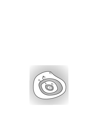
Figure 2: Example of system in which there is a successive embedding of conductors. The volume $V_{S_{T}}$ corresponds to the region in white. The regions corresponding to empty cavities (and their associated surfaces and volumes) can be excluded without affecting the calculations. In this picture cavity A is empty and its surface and volume need not be considered for calculations.

III Some additional properties

We define a function $F$

$$F\equiv\sum_{j=1}^{N+1}f_{j},$$ (14)

and see from Eq. (6) that

$$\nabla^{2}F=0,\qquad F(S_{i})=1\qquad(i=1,\ldots,N+1).$$ (15)

Since $F=1$ throughout the surface $S_{T}$, we see by uniqueness that $F=1$ in the volume $V_{S_{T}}$ from which we find that

$$\sum_{j=1}^{N+1}f_{j}=1.$$ (16)

In addition, by summing over $j$ in Eq. (7b) and taking into account Eq. (16), we find that

$$\sum_{j=1}^{N+1}C_{ij}=0\qquad(i=1,\ldots,N+1).$$ (17)

The symmetry of the $C_{ij}$ elements leads also to

$$\sum_{i=1}^{N+1}C_{ij}=0\qquad(j=1,\ldots,N+1).$$ (18)

Equations (17) and (18) imply that the sum of the elements over any row or column of the matrix is zero. Appendix A gives some proofs of consistency for these important properties. Taking into account the symmetrical nature of the $C_{ij}$ matrix with dimensions $(N+1)\times(N+1)$ and the $N+1$ constraints in Eq. (18), we see that for a system of $N$ conductors surrounded by another conductor $N+1$, the number of independent capacitance coefficients is

$$(N+1)^{2}-\left[\frac{N(N+1)}{2}\right]-(N+1)=\frac{N(N+1)}{2},$$ (19)

Other important properties are that

$$C_{ii} \geq 0$$ (20a)

$$C_{ij} \leq 0,\qquad(i\neq j).$$ (20b)

Equation (20a) follows straightforwardly from Eq. (10). To demonstrate Eq. (20b), we recall that the solutions of Laplace’s equation cannot have local minima nor local maxima in the volume in which the equation is valid.Berkeley ; Jack Consequently, the $$f_{j}$$ functions must lie in the interval

$$0\leq f_{j}\leq 1.$$ (21)

Because $f_{j}=0$ on any surface $S_{i}$ for $i\neq j$, we see that $f_{j}$ acquires its minimum value on such surfaces. Therefore the function $\nabla f_{j}$ should point outward with respect to the conductor $i$ for $i\neq j$. Hence

$$\mathbf{n}_{i}\cdot\nabla f_{j}\geq 0\ \mbox{for}\ i\neq j.$$ (22)

We substitute Eq. (22) into Eq. (7) and obtain $C_{ij}\leq 0$ for $i\neq j$. An additional derivation of the fact that $C_{ii}\geq 0$ can be obtained by taking into account that $f_{j}$ acquires its maximum value on the surface $S_{j}$.

Equation (18) can be rewritten as

$$\sum_{i=1}^{N}C_{ij}=-C_{N+1,j}.$$ (23)

From Eq. (20) we have that $C_{N+1,j}\leq 0$ for $j=1,\ldots,N$ and $C_{N+1,N+1}\geq 0$. Hence

$$\sum_{i=1}^{N}C_{ij} \geq 0\qquad(j=1,\ldots,N)$$ (24a)

$$\sum_{i=1}^{N}C_{i,N+1} \leq 0.$$ (24b)

The following properties follow from Eqs. (11), (18), (20), and (24)

$$|C_{ii}| \geq\sum_{i\neq j}^{N}|C_{ij}|$$ (25a)

$$|C_{ii}| \geq|C_{ij}|,$$ (25b)

$$C_{ii}C_{jj} \geq C_{ij}^{2}$$ (25c)

$$|C_{N+1,N+1}| =\sum_{i=1}^{N}|C_{i,N+1}|$$ (25d)

$$|C_{N+1,N+1}| \geq|C_{i,N+1}|,$$ (25e)

where $$i,j=1,\ldots,N$$.

A particularly interesting case arises when the external conductor is at zero potential. In such a case, although the elements of the form $C_{N+1,j}$ do not necessarily vanish, they do not appear in the contributions to the charge on the internal conductors as can be seen from Eq. (7) by setting $\varphi_{N+1}=0$. For this reason, the capacitance matrix used to describe $N$ free conductors (that is, not surrounded by another conductor) has dimensions $N\times N$.note3

IV Two conductors

We illustrate our method by deriving the basic properties of a system of two conductors. These examples will show the usefulness of Eq. (7) and some of the properties derived from our approach. We analyze a single internal conductor with an external conductor that is, $N=1$. The internal conductor is labeled as conductor 1. From Eqs. (11) and (18) we have

$$C_{21}=C_{12}=-C_{11}=-C_{22}.$$ (26)

Therefore, there is only one independent coefficient, say $C_{11}$ (in agreement with Eq. (19) with $N=1$). The charges on the internal and external conductors can be calculated from Eq. (7)

$$Q_{1} =C_{11}(\varphi_{1}-\varphi_{2})$$ (27a)

$$Q_{2} =-C_{11}(\varphi_{1}-\varphi_{2})=-Q_{1}.$$ (27b)

Equation (27b) is consistent with Eq. (43) and shows that the charge induced on the surface of the cavity of the conductor 2 is opposite to the charge on the conductor 1.

In Table 1 we display the results of three well known configurations of two conductors. The second column shows the $f_{i}$ functions, which can be found by Laplace’s equation (6) and used to calculate $C_{11}$ with Eq. (7).

System	$f_{1}$	$C_{11}$
Spherical shell with radius $b$ and concentric solid sphere with radius $a$.	$\frac{ab}{b-a}\left(\frac{1}{r}-\frac{1}{b}\right)$	$\frac{4\pi\varepsilon_{0}ab}{b-a}$
Cylindrical shell with radius $b$ and concentric solid cylinder with radius $a$, both with length $L$.	$\frac{\ln(r/b)}{\ln(a/b)}$	$\frac{2\pi\varepsilon_{0}L}{\ln(b/a)}$
Two parallel planes with area $A$ at $x=0$ and $x=d$ (conductor 1).	$x/d$	$\varepsilon_{0}\frac{A}{d}$

Table 1: $C_{11}$ and $f_{1}$ factors for three systems of two conductors with $a$ $\leq r\leq b$ and $0\leq x\leq d$. We neglect edge effects for the cylinders and planes.

V Examples

We use our approach to study a system with embedded of conductors. In addition, the case of two internal conductors is examined, and we show the limit in which the configuration of two conductors without external conductor is obtained. These examples show how the properties we have derived can be used to calculate the capacitance coefficients.

Example 1. Consider two concentric spherical shells with radii $b$ and $c$ and a solid spherical conductor (concentric with the others) with radius $a$ such that $c>b>a$. The potentials are denoted by $\varphi_{1}$, $\varphi_{2}$, and $\varphi_{3}$ respectively. The general solution of Laplace’s equation for $f_{i}$ can be written as

$$f_{i}=\frac{A_{i}}{r}+B_{i}.$$ (28)

From Eqs. (6) and (28) we obtain $f_{1}$ and $f_{3}$

$$f_{1}=\begin{cases}\frac{ab}{b-a}\Big{(}\frac{1}{r}-\frac{1}{b}\Big{)}&(a\leq r\leq b)\\ 0&(b\leq r\leq c)\end{cases}$$ (29)

$$f_{3}=\begin{cases}0&(a\leq r\leq b)\\ \frac{bc}{c-b}\left(\frac{1}{b}-\frac{1}{r}\right)&(b\leq r\leq c)\end{cases}.$$ (30)

Although $f_{2}$ can be obtained the same way, it is easier to extract it from Eq. (16). The result is

$$f_{2}=\begin{cases}\frac{ab}{b-a}\left(\frac{1}{a}-\frac{1}{r}\right)&(a\leq r\leq b)\\ \frac{bc}{c-b}\left(\frac{1}{r}-\frac{1}{c}\right)&(b\leq r\leq c)\end{cases}.$$ (31)

The nine capacitance coefficients can be evaluated explicitly from Eq. (7), but it is easier to use Eqs. (11) and (18) and to take into account that $C_{31}=0$ ($\nabla f_{1}(r)=0$ for $r>b$). We have

$$C_{13} =0, C_{12}=-C_{11}$$ (32a)

$$C_{22} =C_{11}-C_{32}, C_{33}=-C_{32}.$$ (32b)

From Eq. (7) the charge on each conductor is

$$Q_{1} =C_{11}(\varphi_{1}-\varphi_{2})$$ (33a)

$$Q_{2} =-Q_{1}+C_{32}(\varphi_{3}-\varphi_{2})$$ (33b)

$$Q_{3} =C_{32}(\varphi_{2}-\varphi_{3})=-(Q_{1}+Q_{2}).$$ (33c)

Hence, we only have to calculate $$C_{11} C_{32}$$ and . note4 The result gives

$$C_{11}=4\pi\varepsilon_{0}\frac{ab}{b-a},\quad C_{32}=-4\pi\varepsilon_{0}\frac{bc}{c-b}.$$ (34)

If $\varphi_{2}=\varphi_{3}$, we find that $Q_{1}=-Q_{2}$ and $Q_{3}=0$. It can be shown that Eqs. (32) and (33) are valid even if the conductors are neither spherical nor concentric, because those equations come from Eqs. (7a), (11), and (18) which are general properties independent of specific geometries.

Example 2. Consider two internal conductors and a grounded external conductor. As customary, we begin with $Q_{1}=Q_{2}=0$. By transfering charge from one internal conductor to the other we keep $Q_{1}=-Q_{2}$. From Eq. (7a) and defining $V\equiv\varphi_{1}-\varphi_{2}\$we find

$$Q_{1} = \left(C_{11}+C_{12}\right)\varphi_{1}-C_{12}V,$$ (35)

$$Q_{1} = -C_{13}\varphi_{1}-C_{12}V,$$ (36)

where we have used Eq. (18). Similarly $Q_{2}=-C_{23}\varphi_{1}-C_{22}V$, and using again Eq. (18) we find

$$Q_{1}+Q_{2}=C_{33}\varphi_{1}-C_{32}V.$$ (37)

Since the system is neutral $Q_{1}+Q_{2}=0$ and hence

$$\varphi_{1}=-\frac{C_{32}}{C_{33}}V,$$ (38)

substituting Eq. (38) into Eq. (36) we obtain

$$Q_{1}=CV\ \ \ ;\ \ \ C\equiv\frac{C_{13}C_{32}-C_{33}C_{12}}{C_{33}}.$$ (39)

Because $N=2$ only three of the coefficients in the definition of $C$ are independent. From Eqs. (20) we see that this effective capacitance is non negative. The procedure is not valid if $C_{33}=0$, in that case we see by using Eqs. (18) and (20) that $C_{i3}=C_{3i}=0$, and from Eq. (36) we find $C=-C_{12}=C_{22},$ which is also non negative. The limit in which there is no external conductor is obtained by taking all the dimensions of the cavity to infinity while keeping the external conductor grounded as discussed in Ref. note3, .

VI Conclusions

We have used an approach based on Laplace’s equation to demonstrate that the capacitance matrix depends only on purely geometrical factors. The explicit use of Laplace’s equation permits us to demonstrate many properties of the capacitance coefficients. The geometrical relations and properties shown here permits us to simplify many calculations of the capacitance coefficients. We emphasize that Laplace’s equations necessary for finding the capacitance coefficients are purely geometrical as can be seen from Eqs. (6) and (7). Laplace’s equation is usually easier than Green function formalism for either analytical or numerical calculations. Appendix A shows some proofs of consistency to enhance the physical insight and the reliability of our method.

Appendix A Proofs of consistency

A proof of consistency for the identity (18), is achieved by using Eq. (7) to calculate the total charge on the $N$ internal conductorsnote5

$$Q_{\mathrm{int}}=\sum_{i=1}^{N}Q_{i}=\sum_{j=1}^{N+1}\left[\varphi_{j}\sum_{i=1}^{N}C_{ij}\right].$$ (40)

We use Eq. (18) to find

$$Q_{\mathrm{int}}=-\sum_{j=1}^{N+1}C_{N+1,j}\varphi_{j}.$$ (41)

Note that Eq. (41) requires many fewer elements of the $C_{ij}$ matrix than Eq. (40). This difference becomes more significant as $N$ increases. If we again use Eq. (7), we can find the charge on the cavity of the external conductor

$$Q_{N+1}=\sum_{j=1}^{N+1}C_{N+1,j}\varphi_{j},$$ (42)

and therefore

$$Q_{N+1}=-Q_{\mathrm{int}},$$ (43)

a property that can also be obtained from Gauss’s law. Berkeley ; Jack

Another proof of consistency for Eq. (18) is found by employing Eqs. (7) and (41) to calculate $Q_{\mathrm{int}}$ (taking into account that Eq. (41) comes directly from Eq. (18))

$$Q_{\mathrm{int}} =-\sum_{j=1}^{N+1}C_{N+1,j}\varphi_{j}$$ (44a)

$$=\varepsilon_{0}\oint_{S_{N+1}}\nabla\left(\sum_{j=1}^{N+1}f_{j}\varphi_{j}\right)\cdot\mathbf{n}_{N+1}\,dS.$$ (44b)

We utilize Eq. (5) to write $$Q_{\mathrm{int}}$$ as

$$Q_{\mathrm{int}}=\varepsilon_{0}\!\oint_{S_{N+1}}\nabla\phi\cdot\mathbf{n}_{N+1}\,dS=\varepsilon_{0}\oint_{S_{N+1}}\mathbf{E}\cdot(-\mathbf{n}_{N+1})\,dS.$$ (45)

This relation is clearly correct because $\mathbf{n}_{N+1}$ points inward with respect to the volume $V_{S_{T}}$.

A proof of consistency for Eq. (10) that shows the symmetry of $C_{ij}$ can be obtained by calculating the electrostatic internal energy, which in terms of the electric field is

$$U =\frac{\varepsilon_{0}}{2}\!\int_{V_{S_{T}}}E^{2}\,dV=\frac{\varepsilon_{0}}{2}\int_{V_{S_{T}}}\mathbf{\nabla}\phi\cdot\mathbf{\nabla}\phi\,dV$$ (46a)

$$=\frac{1}{2}\sum_{i,j}^{N+1}\varphi_{i}\varphi_{j}\left[\varepsilon_{0}\int_{V_{S_{T}}}\mathbf{\nabla}f_{i}\cdot\mathbf{\nabla}f_{j}\,dV\right],$$ (46b)

where we have used Eq. (5). From Eq. (10) we find

$$U=\frac{1}{2}\sum_{i,j}^{N+1}C_{ij}\varphi_{j}\varphi_{i}=\frac{1}{2}\sum_{i}^{N+1}Q_{i}\varphi_{i},$$ (47)

consistent with standard results.Berkeley ; Jack

Appendix B Suggested Problems

To enhance the understanding of this approach and its advantages, we give some general suggestions for the reader.

1. Implement a numerical method to solve the Laplace’s equation (6) for the $f_{i}$ functions associated with a nontrivial geometry (for example, two non-concentric ellipsoids). Use Eqs. (16) and (21) to either simplify your calculations or to check the consistency of your results. Then use Eq. (7) to obtain the $C_{ij}$ factors numerically. Use Eq. (11) and Eqs. (17)–(25) either to simplify your calculations or to check the consistency of your results.

2. We have emphasized that to calculate the total charge on the internal conductors Eq. (41) requires many fewer $C_{ij}$ elements than Eq. (40). How many fewer elements are required for an arbitrary value of $N$?

3. For a successive embedding of concentric spherical shells, calculate the capacitance coefficients for an arbitrary number of spheres.

4. Show that for the successive embedding of three conductors with arbitrary shapes, Eqs. (32) and (33) still hold. Generalize your results for an arbitrary number of conductors.

- (1) W. Taussig Scott, The Physics of Electricity and Magnetism (John Wiley & Sons, New York, 1966), 2nd ed.; Gaylord P. Harnwell, Principles of Electricity and Electromagnetism (McGraw-Hill, New York, 1949); Leigh Page and Norman I. Adams Jr., Principles of Electricity (D. Van Nostrand, New Jersey, 1958), 3rd ed.; A. N. Matveev, Electricity and Magnetism (Mir, Moscow, 1988).
- (2) J. D. Jackson, Classical Electrodynamics (John Wiley & Sons, New Jersey, 1998), 3rd ed.; David J. Griffiths, Introduction to Electrodynamics (Prentice Hall, New Jersey, 1999), 3rd ed.
- (3) Mituo Uehara, “Green’s functions and coefficients of capacitance,” Am. J. Phys. 54 (2), 184–185 (1986).
- (4) V. Lorenzo and B. Carrascal, “Green’s functions and symmetry of the coefficients of a capacitance matrix,” Am. J. Phys. 56 (6), 565 (1988).
- (5) C. Donolato, “Approximate evaluation of capacitances by means of Green’s reciprocal theorem,” Am. J. Phys. 64 (8), 1049–1054 (1996).
- (6) Y. Cui, “A simple and convenient calculation of the capacitance for an isolated conductor plate,” Eur. J. Phys. 17 (6), 363–364 (1996).
- (7) E. Bodegom and P. T. Leung, “A surprising twist to a simple capacitor problem,” Eur. J. Phys. 14 (2), 57–58 (1993).
- (8) G. P. Tong, “Electrostatics of two conducting spheres intersecting at angles,” Eur. J. Phys. 17 (4), 244–249 (1996).
- (9) is not necessarily the total charge on the external conductor, but the charge accumulated on the surface of the cavity that encloses the other conductors. The value of the charge is calculated with the surface integral (2), which for the case of the internal conductors encompasses the whole surface, but for the external conductor is only the surface of the cavity that encloses the other conductors.
- (10) Equation (10) is an integral over the volume for the factors. We might be tempted to use Gauss’ theorem to obtain an integral of the volume directly from Eq. (7). However, is not defined in the region inside the conductors. The gradient of in Eq. (7) is evaluated in an external neighborhood of the conductor surface.
- (11) By uniqueness, the solution for this problem is equivalent to the solution for a system consisting of the same conductors contained in the cavity of a surrounding conductor, such that all the dimensions of the cavity tend to infinity, and the potential of the external conductor is set to zero.
- (12) If we take into account that is another degree of freedom (although zero), we have a total of three degrees of freedom, in agreement with Eq. (19) for .
- (13) For a derivation of some of these results based on the energy of the electrostatic field see L. D. Landau, E. M. Lifshitz, and L. P. Pitaevskii, Electrodynamics of Continuous Media (Elsevier Butterworth-Heinemann, 1984), 2nd ed., p. 3.