Random RNA under tension

Abstract

The Lässig-Wiese (LW) field theory for the freezing transition of random RNA secondary structures is generalized to the situation of an external force. We find a second-order phase transition at a critical applied force $f=f_{c}$. For $f<f_{c}$ forces are irrelevant. For $f>f_{c}$, the extension $\cal L$ as a function of pulling force $f$ scales as ${\cal L}(f)\sim(f-f_{c})^{1/\gamma-1}$. The exponent $\gamma$ is calculated in an $\epsilon$-expansion: At 1-loop order $\gamma=\epsilon/2=1/2$, equivalent to the disorder-free case. 2-loop results yielding $\gamma=0.6$ are briefly mentioned. Using a locking argument, we speculate that this result extends to the strong-disorder phase.

1 Introduction

RNA is a heteropolymer constructed from four different nucleotides A, C, G and U located on a sugar-phosphate polymer backbone. In solution, a single RNA strand bends back onto itself and folds into a configuration of loops, stems and terminating bonds, due to formation of Watson-Crick pairs A-U and C-G from bases located on different parts of the strand. Together with environmental conditions like temperature and ionic concentration, the primary structure (base sequence) determines the most probable base-pairings, known as secondary structure, which then determines the most probable spatial conformation (tertiary structure) [1, 2]. Unlike protein folding, which exhibits a strong interdependence between secondary and tertiary structure [3], RNA folding may be studied at the level of secondary structures due to a clear separation of energy scales.

Since the pioneering work of Bundschuh and Hwa [4], several authors have studied the statistical physics of RNA secondary structures for random sequences [5, 6, 7, 8]. It is commonly believed that these systems undergo a freezing transition upon lowering the temperature. Based on a replica approach, Lässig and Wiese [9], and David and Wiese [10] have recently developed a systematic field-theory formulation for this phase transition in terms of interacting random walks (RW). The critical exponents characterizing pairing statistics and replica overlap were computed within a 2-loop renormalization analysis, and found to be remarkably close to numerical simulations [4, 11].

An interesting way to probe RNA chains is to study its behavior under an external pulling force (see fig. 1a for an illustration). Recently, force-extension curves have been measured, by attaching beads to the RNA-molecule and pulling on it, using an optical trap [12, 13]. For homopolymers, the competition between structure formation and denaturation of the RNA strand leads to a second-order phase transition at a critical force $f=f_{c}$ [11]. For $f<f_{c}$ the strand is still in a collapsed phase, while for $f>f_{c}$ it is in a extended “necklace phase” with a macroscopic extension (end-to-end distance). While quite some literature exists about the subject (see e.g. [14, 15]) there is of today no theory to compute the characteristic exponent $\gamma$ of the force-extension characteristics for disordered RNA strands at the transition. In this letter we fill this gap. We propose an extension of the RW field theory for random RNA by including an external pulling force $f$. We show that within our theory the force is renormalized by the quenched disorder, hence the exponent $\gamma$ is modified with respect to its mean-field value $\gamma_{0}=1/2$. Conversely, we argue that the disorder coupling is not renormalized by the force at any order in perturbation theory. We use perturbative renormalization of the new theory to compute $\gamma$ to 1-loop order. Finally, we comment on 2-loop results.

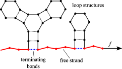
	(a)
	(b)
	(c)

Figure 1: (a) Illustration of the planar structure of RNA under tension, (b) rainbow diagram and (c) corresponding height relief.

2 The model

We consider an RNA strand with $L$ bases labeled with indices $s=1,\dots,L$. Similarly, we use the index $s$ to label a backbone segment between adjacent bases $s$ and $s+1$. A secondary structure $S$ is a set of base pairs $(s,t),\,s<t$. We only retain so-called planar structures $S$: any two different base pairs $(s,t)$, $(s^{\prime},t^{\prime})$ are either independent $s<t<s^{\prime}<t^{\prime}$ or nested $s<s^{\prime}<t^{\prime}<t$. $S$ can be represented by a diagram of arches (fig. 1b). Planarity implies that the arches do not cross each other. We introduce the contact operator $\Phi$ defined by $\Phi(s,t)=1$ if $(s,t)\in S$, and $0$ otherwise [9]. Moreover we define the height field $h$ on the segment $r$ by $h(r):=\sum_{s\leq r}\sum_{t>r}^{L}\Phi(s,t)$, counting the number of arches over $r$. This leads to an identification of each open planar secondary structure $S$ with a height function subject to boundary conditions $h(0)=h(L)=0$. A segment between the bases $r$ and $r+1$ belongs to the free part of the structure if and only if $h(r)=0$ (fig. 1c).

In order to develop a statistical mechanics model, we have to assign to each structure $S$ an energy $E[S]$. We assume that it may be written as a sum of the contributions from the formation of base pairs $E_{\mathrm{pair}}[S]$ and from the external force $E_{\mathrm{force}}[S]$. Bond formation between the bases at $s$ and $t$ involves a pairing energy $\eta(s,t)$ which in general depends on the nature of the pairing partners. We sum over all pairing energies of base pairs in $S$ and obtain $E_{\mathrm{pair}}[S]=\sum_{s<t}\eta(s,t)\Phi(s,t)$ [4]. The energy due to the external force, $E_{\mathrm{force}}[S]$, depends on the spatial configuration of the free part of the strand and its elasticity. We assume that every free backbone segment aligns with the force, hence the energy is proportional to the force $f$ times the number of monomers in the free strand [6]. Thus, we neglect any elasticity and entropic effects for the free segments and for the bonds which terminate loop structures (figure 1a). By analogy with the contact operator $\Phi(s,t)$, we introduce a free-strand operator $\Delta(r)$ such that $\Delta(r)=1$ if $h(r)=0$, and $0$ otherwise. This allows to write $E_{\mathrm{force}}[S]=-f\sum_{r}\Delta(r)\ .$

Having defined the energy of a given secondary structure, we proceed to study the partition function

$$Z=\sum_{S\in\mathcal{S}(L)}\exp\left[-\sum_{s<t}\eta(s,t)\Phi(s,t)+f\sum_{s}\Delta(s)\right]$$ (1)

where $\mathcal{S}(L)$ denotes the set of all possible planar secondary structures with $L$ bases. Before considering random RNA chains, we briefly review the properties of the partition function in the case of uniform pairing energies $\eta(s,t)=\eta_{0}$ (that we may take $=0$). For $f=0$ one deduces from the height picture that the problem is equivalent to the statistics of a RW on the positive real axis $h\geq 0$. The partition function is $Z_{L}\propto L^{-\rho_{0}}$ with $\rho_{0}=3/2$ the characteristic exponent of first return. This leads to a pairing probability for the base pair $(s,t)$ scaling like $p(s,t)=\langle\Phi(s,t)\rangle\propto[|t-s|(L-|t-s|)]^{-\rho_{0}}$. Switching on the force $f>0$ amounts to adding an attractive short-range potential at the origin $h=0$. This is a well-known problem of statistical mechanics. For instance it describes surface wetting transitions in $1+1$ dimensions (see e.g. [16]). For forces $f$ larger than a critical force $f_{c}$, the RW is bound to the origin $h=0$ whereas for $f<f_{c}$ it is unbound (i.e. free to wander far away from $h=0$).

In fact, the $f=0$ problem can be mapped onto a free RW $\vect{r}(s)$ in $d=2\rho_{0}=3$ dimensions; the height field is the modulus $h(s)=|\vect{r}(s)|$. The inclusion of the short-ranged attraction in the case $f>0$ corresponds to a short-ranged attractive potential at $\vect{r}=0$. In the continuum limit, the action of this model reads

$$S_{3D}[\vect{r}(s)]=\int_{0}^{L}\upd s\,\left(\frac{1}{4}\left[\dot{\vect{r}}(s)\right]^{2}-f\delta^{3}(\vect{r}(s))\right)\ ,$$ (2)

and describes the pinning of a RW by an attractive impurity at the origin.

We now exploit this analogy to extend our analysis to random RNA structures. Numerical simulations [4] suggest to model sequence disorder by independent Gaussian random binding energies $\eta(s,t)$,

$$\overline{\eta(s,t)}=\eta_{0}\ ,\ \ \overline{\eta(s,t)\eta(u,v)}-\eta_{0}^{2}=\sigma^{2}\delta(s-u)\delta(t-v)$$ (3)

Following [9, 10], we construct a field theory in the continuum limit $L\rightarrow\infty$. We perform a perturbative expansion in the disorder amplitude $g=\sigma^{2}>0$, and the force strength $f$. To model disorder, we use the replica trick. Each replica $\alpha=1,\dots,n$ is represented by a RW $\vect{r}_{\alpha}(s)$ in an embedding space $\mathbb{R}^{d}$ (with dimension $d=2\rho_{0}=3$). In fact, the explicit form of the pairing probability for uniform RNA suggests to consider closed RWs $\vect{r}_{\alpha}(s)$. Nevertheless, we can (and shall) use open RWs because they have been proven to lie in the same universality class and considerably simplify the calculations [10]. Within the RW representation, the contact operator reads $\Phi_{\alpha}(s,t)=\delta^{d}(\vect{r}_{\alpha}(s)-\vect{r}_{\alpha}(t))$. The average over the disorder $\eta$ generates an attractive interaction between the replicas. It is described by the overlap operator $\Psi_{\alpha\beta}(s,t)=\Phi_{\alpha}(s,t)\Phi_{\beta}(s,t)$ (counting the common arches of the replicas $\alpha$ and $\beta$ in the original picture). By analogy with (2) we represent the operator $\Delta$ as $\Delta_{\alpha}(s):=\delta^{d}(\vect{r}_{\alpha}(s))$. The resulting action in the RW picture is

$$S[\{\vect{r}_{\alpha}\}]=\sum_{\alpha}\int\frac{1}{4}\left[\dot{\vect{r}}_{\alpha}(s)\right]^{2}\\ -g\sum_{\alpha<\beta}\iint_{s<t}\Psi_{\alpha\beta}(s,t)-f\sum_{\alpha=1}^{n}\int\Delta_{\alpha}(s)\ ,$$ (4)

and generalizes the model of [10] (where $f=0$). Before using perturbation theory, we generalize the model to dimensions $2\leq d\leq 3$ [9, 10]. Setting $\epsilon=d-2$ we find the canonical scaling dimensions $\text{dim}\,g=\epsilon$ and $\text{dim}\,f=\epsilon/2$. The original theory corresponds to $\epsilon=1$. The generalized model is renormalizable at $\epsilon=0$ as the $f=0$ model [17].

3 Perturbation theory

We represent the perturbative expansion of $Z$ in $f,\,g$ in terms of Feynman diagrams. The $g$-vertex $\Psi_{\alpha\beta}$ (disorder interaction vertex) is denoted by a double arch between a pair of replicas [9, 10] and the $f$-vertex $\Delta_{\alpha}$ (force interaction at $r=0$) is depicted by a force insertion on a single replica:

$$\Psi_{\alpha\beta}\ =\ \includegraphics[height=28.45274pt]{figure2}\qquad\Delta_{\alpha}\ =\ \includegraphics[height=28.45274pt]{figure3}$$ (5)

Non-planar diagrams involving the disorder interaction, see fig. 2(a), may be eliminated by introducing $n\times N$ pairs of auxiliary fields $\gamma$ and $\tilde{\gamma}$ in the action and by taking the large-$N$ limit [10]. Since the force term only acts on the free part of the RNA strand, also diagrams of the type given on fig. 2(b) must be excluded. This is achieved by a similar “planarity constraint” that can be implemented using the same auxiliary fields.

(a)	(b)

Figure 2: Non-planar diagrams.

We now consider the partition function for a single (bundle of replica) RW with fixed end-points, or rather its Fourier transform $Z(\{\vect{q}_{\alpha}^{\prime}\},\{\vect{q}_{\alpha}^{\prime\prime}\};f,g)$, defined as

$$Z(\{\vect{q}_{\alpha}^{\prime},\vect{q}_{\alpha}^{\prime\prime}\};f,g)\\ =\int\mathcal{D}[\{\vect r_{\alpha}\}]\,\mathrm{e}^{-S[\{\vect r_{\alpha}\}]}\,\prod_{\alpha}V_{\vect q^{\prime}_{\alpha}}^{\alpha}(0)V_{\vect q^{\prime\prime}_{\alpha}}^{\alpha}(L)$$ (6)

where the vertex operator $V_{\vect q}^{\alpha}(s)=\exp\left(i\vect q\vect r_{\alpha}(s)\right)$ injects incoming external momenta $\{\vect{q}_{\alpha}^{\prime}\},\{\vect{q}_{\alpha}^{\prime\prime}\}$ to each end-point of the replica $\alpha$ of the RW. The (regularized) dimensionless integration measure is given by $\mathcal{D}[\vect{r}_{\alpha}]=\prod_{i}\upd^{d}\vect{r}_{\alpha,i}/(4\pi a^{2}/m)^{d/2}$ where $a$ is an ultraviolet cut-off and $m=1/2$ the mass of the Brownian particle associated with the RW. We further simplify the model by setting $\vect{q}_{\alpha}^{\prime}\equiv\vect{q}^{\prime},\,\vect{q}_{\alpha}^{\prime\prime}\equiv\vect{q}^{\prime\prime}$ without loss of generality.

The perturbative expansion in $g$ and $f$ leads to a systematic diagrammatic representation of $Z$. The diagrams can be classified according to the number of replicas with force insertions. The absence of force insertions on the replica $\alpha$ leads to a momentum conservation $\delta^{d}(\vect{q}^{\prime}_{\alpha}+\vect{q}^{\prime\prime}_{\alpha})$ (translation invariance $\vect r_{\alpha}(s)\to\vect r_{\alpha}(s)+\vect r$). Thus, the set of all possible diagrams is classified according to the number $k$ of its external momentum conservations: $k=n$ conservations correspond to a diagram of the force-free theory, $k=n-1$ conservations to a single replica subject to force insertions, etc. We group all diagrams with $k$ conservations into a restricted partition function $\Xi_{n-k}(\vect{q}^{\prime},\vect{q}^{\prime\prime};f,g)$, so that formally $Z(\vect{q}^{\prime},\vect{q}^{\prime\prime};f,g)=\sum_{k}\delta(\vect{q}^{\prime}+\vect{q}^{\prime\prime})^{k}\Xi_{n-k}(\vect{q}^{\prime},\vect{q}^{\prime\prime};f,g)$. $\Xi_{0}$ describes the force-free theory, $\Xi_{1}$ the sector where the attractive short-range potential only acts upon a single replica, $\Xi_{2}$ the sector where it acts upon two replicas, etc. In the following we focus on $\Xi_{1}(\vect q,-\vect q)$, since this simplifies the calculations. Perturbative expansion up to order two in $f$ or $g$ yields

$$\Xi_{1}(\vect q,-\vect q;f,g)=$$

$$\ f\,n\,\includegraphics[height=28.45274pt]{figure5}\,+\,f^{2}\,n\,\includegraphics[height=28.45274pt]{figure6}$$

$$+\,fg\Bigg{[}n(n-1)\,\bigl{(}\ \includegraphics[height=28.45274pt]{figure7}+\includegraphics[height=28.45274pt]{figure8}\bigr{)}$$

$$\qquad~{}~{}~{}+\frac{n(n-1)(n-2)}{2}\ \includegraphics[height=28.45274pt]{figure9}\Bigg{]}\,+\,\cdots$$ (7)

There are four topologically different Feynman diagrams. The first contribution is

$$=\underset{0<u<L}{\int}\hskip-5.0pt\langle{\Delta_{1}(u)\prod_{\alpha=1}^{n}V_{\vect q}^{\alpha}(0)V_{-\vect q}^{\alpha}(L)}\rangle_{0}$$

$$=\ L\,e^{-{\vect q}^{2}Ln},$$ (8)

where $\langle\quad\rangle_{0}$ denotes the average w.r.t. the free RW action $S_{0}[\vect r]$ ($f=g=0$), with a proper subtraction of the $(n-1)$ translational zero-modes. The second diagram is UV divergent at $\epsilon=0$. Isolation of the corresponding pole yields

$$=\underset{0<u<v<L}{\iint}\hskip-5.0pt\langle{\Delta_{1}(u)\Delta_{1}(v)\prod_{\alpha=1}^{n}V_{\vect q}^{\alpha}(0)V_{-\vect q}^{\alpha}(L)}\rangle_{0}$$

$$\ =\ \underset{0<u<v<L}{\iint}e^{-\vect q^{2}(L-v+u)}|v-u|^{-d/2}e^{-\vect q^{2}L\,(n-1)}$$

$$\mathop{=}_{\epsilon\to 0}\ -\frac{L^{2}}{\epsilon}\,e^{-{\vect q}^{2}Ln}+O(1)$$ (9)

The divergence comes from the short-distance behavior of the product of two $\Delta$ operators $\Delta(u)\Delta(v)\mathop{=}\limits_{u\to v}|u-v|^{-d/2}\Delta(v)+\cdots$. The third contribution is also UV divergent,

$$\includegraphics[height=28.45274pt]{figure7}=\includegraphics[height=28.45274pt]{figure8}$$

$$=\underset{0<u<v<w<L}{\iiint}\langle{\Delta_{1}(u)\Psi_{12}(v,w)\prod_{\alpha=1}^{n}V_{\vect q}^{\alpha}(0)V_{-\vect q}^{\alpha}(L)}\rangle_{0}$$

$$=\underset{0<u<v<w<L}{\iiint}e^{-2\vect q^{2}(L-w+v)}|w-v|^{-d}e^{-\vect q^{2}L\,(n-2)}$$

$$\mathop{=}_{\epsilon\to 0}\ -\frac{L}{\epsilon}\,(L\vect q^{2}-1)\,e^{-{\vect q}^{2}Ln}+O(1)\ ,$$ (10)

as well as the fourth

$$=\underset{\begin{subarray}{c}0<u<L\\ 0<v<w<L\end{subarray}}{\iiint}\langle{\Delta_{1}(u)\Psi_{23}(v,w)\prod_{\alpha=1}^{n}V_{\vect q}^{\alpha}(0)V_{-\vect q}^{\alpha}(L)}\rangle_{0}$$

$$=\ \underset{\begin{subarray}{c}0<u<L\\ 0<v<w<L\end{subarray}}{\iiint}e^{-2\vect q^{2}(L-w+v)}|w-v|^{-d}e^{-\vect q^{2}L\,(n-2)}$$

$$\mathop{=}_{\epsilon\to 0}-\frac{L}{\epsilon}\,(2L\vect q^{2}-1)\,e^{-{\vect q}^{2}Ln}+O(1)\ .$$ (11)

4 Renormalization

We remove the UV divergences in the expansion (3) by formally taking $\rho_{0}$ as analytical regularization parameter. In order to eliminate the simple poles in $\epsilon=2\rho_{0}-2$ at $\epsilon=0$, we define the renormalized theory through the renormalized action

$$S_{R}=\sum_{\alpha}\int_{s}\frac{\mathbb{Z}}{4}\dot{\vect{r}}^{2}_{\alpha}-g_{R}\mu^{-\epsilon}\mathbb{Z}_{g}\sum_{\alpha<\beta}\underset{0<s<t<L}{\iint}\Psi_{\alpha\beta}(s,t)\\ -f_{R}\mu^{-\epsilon/2}\mathbb{Z}_{f}\int_{s}\Delta_{\alpha}(s)+2n\mathbb{Z}_{1}\ .$$ (12)

Here $\mathbb{Z}$, $\mathbb{Z}_{g}$ and $\mathbb{Z}_{f}$ denote the wave-function, the coupling constant and the force counterterms respectively. $\mathbb{Z}_{1}$ accounts for boundary effects since we deal with open RWs [10]. The coefficients of their development in $f_{R},\,g_{R}$ contain the leading poles in $1/\epsilon$. Furthermore, we have introduced the renormalization mass scale $\mu\sim 1/L$. From dimensional analysis we deduce the relations between renormalized and bare $\vect{r}$, $\vect{q}$, $g$ and $f$: For the field $\vect{r}=\mathbb{Z}^{1/2}\vect{r}_{R}$, $\vect{q}=\mathbb{Z}^{-1/2}\vect{q}_{R}$, for the couplings $g=g_{R}\mu^{-\epsilon}\mathbb{Z}_{g}\mathbb{Z}^{-d}$ and $f=f_{R}\mu^{-\epsilon/2}\mathbb{Z}_{f}\mathbb{Z}^{-d/2}$. The renormalized partition functions are related to the bare ones via

$$\Xi_{k}^{R}(\vect{q}^{\prime}_{R},\vect{q}^{\prime\prime}_{R},f_{R},g_{R})=\mathbb{Z}^{-kd/2}e^{-2n\mathbb{Z}_{1}}\Xi_{k}(\vect{q}^{\prime},\vect{q}^{\prime\prime},f,g)\ .$$ (13)

The prefactor on the r.h.s. takes into account the $(n-k)$ zero modes, boundary effects and the change of normalization in the integration measure. Consistency of the theory requires cancelation of all divergences upon renormalization for each individual $\Xi_{k}$. In particular, renormalization of the force-free terms $\Xi_{0}$ has been performed previously [10] and yields the counter terms $\mathbb{Z}=1+g_{R}(n-1)/\epsilon$, $\mathbb{Z}_{g}=1+g_{R}(7-4n)/\epsilon$ and $\mathbb{Z}_{1}=1+3g(n-1)/4\epsilon$. They do not depend on $f$ at any order since they correspond to “bulk” divergences for the random walk in interaction with the potential at the origin (“boundary” term). For the counter term $\mathbb{Z}_{f}$ we need $\Xi_{1}$, whose Feynman diagrams were computed in eqns. (8)-(3):

$$\Xi_{1}=nLfe^{-(\vect{q}^{\prime})^{2}Ln}\\ \times\left[1+\frac{g(n-1)}{2\epsilon}\left(\frac{n+2}{2}-2n(\vect{q}^{\prime})^{2}L\right)-\frac{2f}{\epsilon}\right].$$ (14)

We absorb the poles by the counter terms of the force-free theory and $\mathbb{Z}_{f}=1+2f/\epsilon$. This expression depends neither on the number of replicas $n$, nor on $g$. Thus at first order there is no coupling between force and disorder. A straightforward calculation gives the RG $\beta$-functions

$$\beta_{f}(g_{R},f_{R}) =-\left.\frac{\upd f_{R}}{\upd\log\mu}\right|_{f}=-\frac{\epsilon}{2}f_{R}+f_{R}^{2},$$ (15)

$$\beta_{g}(g_{R},f_{R}) =-\left.\frac{\upd g_{R}}{\upd\log\mu}\right|_{g}=-\epsilon g_{R}+(5-2n)g_{R}^{2}$$ (16)

In the physical case of random RNA, $n=0$, they yield the RG flow depicted in fig. 3 with four fixed points. The attractive Gaussian fixed point $O=(0,0)$ describes the molten phase of [4]. $D=(\epsilon/5,0)$ is the fixed point of the glass transition found in [9, 10]. We identify $F=(0,\epsilon/2)$ with the denaturation transition of a homopolymer (wetting in $1+1$ dimensions). More interesting, a new bi-critical UV unstable fixed point $B=(\epsilon/2,\epsilon/5)$ emerges from our one-loop analysis. It leads to four phases separated by the critical lines $f\equiv\epsilon/2$ and $g\equiv\epsilon/5$. In particular, a new phase at both high force and strong disorder emerges. Physically, it corresponds to isolated frozen branched structures separated by free parts of the strand.

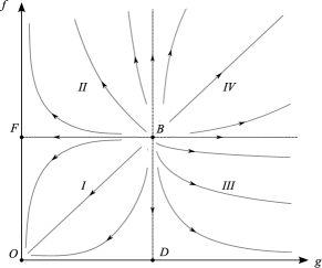
Figure 3: Schematic view of renormalization group flow in the $(g,f)$ plane. The critical lines distinguish the molten phase (I), a glass phase (II), (III) the denatured homopolymer phase. A new phase (IV) corresponds to RNA strands with isolated frozen structures separated by free parts.

The extension ${\cal L}$ as a function of the force $f$ is given by the anomalous dimension of this force. The scaling ansatz reads

$${\cal L}(f)=L^{\alpha}\mathcal{F}\left([f-f_{c}]L^{\gamma}\right)\ ,$$ (17)

where $\mathcal{F}(z)$ is a scaling function. At the bi-critical fixed point, we find

$$\gamma=-\dim[f-f_{c}]=\left.\frac{\partial\beta_{f}}{\partial f_{R}}\right|_{f_{c}}=\frac{\epsilon}{2}\ .$$ (18)

Since ${\cal L}=\left\langle\int_{0}^{L}\mathrm{d}x\,{\Delta(x)}\right\rangle$, the exponent $\alpha=\gamma$. Demanding that for large systems the extension ${\cal L}$ become extensive, i.e. $\sim L$, yields $\mathcal{F}(z)\sim z^{\frac{1}{\gamma}-1}$ for $z\gg 1$, so that for large RNA molecules ${\cal L}(f)\sim L(f-f_{c})^{\frac{1}{\gamma}-1}$. Setting $\epsilon=1$ yields the exponent $\gamma=1/2$ which is the same result as for the homopolymer denaturation transition, first discussed in [11]. This is consistent with the fact that the 1-loop beta function for $f$ does not depend on $g$, so that $\gamma$ is not changed by the quenched disorder. However, this result does not hold at higher orders [17].

5 Conclusion

To summarize, we have developed a field-theoretic description of random RNA under application of an external force, by extending the force-free field theory. It permits to study the second-order denaturation transition. At 1-loop order, the RG flow functions for force $f$ and disorder strength $g$ decouple so that the denaturation is not influenced by disorder. We have computed the critical exponent $\gamma=1/2$ for the force-extension characteristic at the transition which agrees with previously considered homopolymer models.

We have extended our calculations to second order in perturbation theory [17]. The renormalization group flow of $f$ then depends on the disorder strength $g$. The procedure yields a scaling exponent $\gamma=0.6$ for the force-extension characteristic, resulting in ${\cal L}(f)\sim L(f-f_{c})^{\frac{1}{\gamma}-1}\approx L(f-f_{c})^{2/3}$.

We invoke the locking hypothesis [9] in order to conjecture the critical exponents in the glass phase. The argument relies on the exact inequality $dim[\Psi]\geq dim[\Phi]$ for the dimensions of contact and overlap operators. For $\epsilon=1$ consistency of the theory requires that the inequality is satisfied. Physically this means that different replicas follow the same minimal-energy path already at the transition. This is quite unusual. Normally one expects several minimal-energy paths to exist at the transition, and the strong-coupling phase to be characterized by a collapse of these distinct paths into a single one, resulting into different physical exponents. In a situation where at the transition only a single minimal-energy path exists, we cannot have a collapse of several paths, and the accompanying change of critical exponents. In the absence of a different mechanism, the exponents will not change for a small increase in disorder, and by renormalization arguments in the whole strong-coupling phase. We conjecture that this is what happens for the RNA freezing transition. It is then tempting to suppose this hypothesis to hold even in the presence of an external force, i.e. on the critical line beyond the bi-critical fixed point. This assumption leads us to extend our prediction $\alpha=\gamma=0.6$ to the glass phase. Indeed, this prediction proves to be in reasonable agreement with numerical simulations of Müller et al.[11, 18].

- [1] \NameI. Tinoco and C. Bustamante \REVIEWJ. Mol. Biol.2931999271
- [2] \NameP. Higgs \REVIEWQ. Rev. Biophys.332000199
- [3] \NameV.S. Pande, A. Yu. Grosberg and T. Tanaka \REVIEWRev. Mod. Phys.722000259-314
- [4] \NameR. Bundschuh, T. Hwa \REVIEWPhys. Rev. Lett.8319991473, \REVIEWPhys. Rev. E652002031903
- [5] \NameA. Pagnani, G. Parisi and F. Ricci-Tersenghi \REVIEWPhys. Rev. Lett.8420002026
- [6] \NameF. Krzakala, M. Mézard and M. Müller \REVIEWEurophys. Lett.572002752-758
- [7] \NameS. Hui, L.H. Tang e-print q-bio.BM/0608020
- [8] \NameC. Monthus, T. Garel e-print cond-mat/0611611
- [9] \NameM. Lässig and K.J. Wiese \REVIEWPhys. Rev. Lett.962006228101
- [10] \NameF. David and K.J. Wiese e-print q-bio.BM/0607044, accepted for publication in Phys. Rev. Lett.
- [11] \NameM. Müller \REVIEWPhys. Rev. E672003021914
- [12] \NameJ. Liphardt et al. \REVIEWScience2922001733-737, \REVIEWScience29620021832-1835
- [13] \NameB. Onoa et al. \REVIEWScience29920031892-1892
- [14] \NameU. Gerland, R. Bundschuh and T. Hwa \REVIEWBiophys. J.8120011324
- [15] \NameM. Müller, F. Krzakala, and M. Mézard \REVIEWEur. Phys. J. E9200267-77
- [16] \NameM.E. Fisher \BookStatistical Mechanics of Membranes and Surfaces Vol. 5 \EditorD. Nelson, T. Piran, S. Weinberg \PublWorld Scientific \Year1989
- [17] F. David and K.J. Wiese, to be published.
- [18] \NameM. Müller private communication.