Attractors in continuous and Boolean networks

Abstract

We study the stable attractors of a class of continuous dynamical systems that may be idealized as networks of Boolean elements, with the goal of determining which Boolean attractors, if any, are good approximations of the attractors of generic continuous systems. We investigate the dynamics in simple rings and rings with one additional self-input. An analysis of switching characteristics and pulse propagation explains the relation between attractors of the continuous systems and their Boolean approximations. For simple rings, “reliable” Boolean attractors correspond to stable continuous attractors. For networks with more complex logic, the qualitative features of continuous attractors are influenced by inherently non-Boolean characteristics of switching events.

I Introduction

Complex networks of interacting elements arise in many biological, chemical, sociological, and physical contexts. An important example is the network of interactions among proteins and DNA in a cell. The binding of certain proteins to each other and to promoter regions of DNA can create a combinatorially complex logic of gene expression. It is tempting to think of transcriptional networks and similar examples as effectively Boolean in nature. In such a picture, genes are turned “on” and “off” in the presence of proteins produced when other genes are turned on or off Davidson (2006), and many studies of the fundamental principles governing networks of interacting genes have focused Boolean models. Recent work has highlighted distinctions in the attractor structures as network architecture parameters are varied, different distributions of Boolean functions are incorporated, and/or different updating schemes are employed Aldana-Gonzalez et al. (2003); Aldana and Cluzel (2003); Greil and Drossel (2005); Moreira and Amaral (2005); Kesseli et al. (2006); Paul et al. (2006); Samuelsson and Socolar (2006).

The Boolean models are generally understood to be idealized representations of underlying continuous and perhaps stochastic processes, so it is important to understand any artifacts introduced in Boolean approximations. Here we investigate some continuous, deterministic systems motivated by models of transcriptional interactions and designed to be good candidates for a Boolean analysis. The goal is to elucidate the most important effects that may lead the continuous dynamics to differ qualitatively from expectations based on the Boolean models.

We investigate the temporal structure and stability of the attractors of continuous dynamical systems and those of the corresponding Boolean models. Two effects are found to be crucial for understanding the structure of the continuous attractors: first, when an on-off symmetry of typical Boolean models is broken, the possibility of stable pulse propagation down a chain can be lost; and second, the memory of past inputs at a given node causes shifts in the temporal spacing between multiple pulses on a feedback loop. These effects make it difficult to put the attractors of the continuous network into correspondence with the attractors of their Boolean counterparts.

We study rings of $N$ elements (Fig. 1) governed by delay differential equations. The delays are introduced to represent intermediate steps in the process mediating the interactions between elements. We employ a form developed originally as a mean-field description of the dynamics of transcription factor expression Andrecut and Kauffman (2006), though for present purposes it simply provides a generic model of elements with sigmoidal responses to their inputs:

$${\dot{x}}_{j}(t) =f_{j}\boldsymbol{(}x_{j-1}(t-\tau)\boldsymbol{)}-x_{j}(t)\,,$$ (1)

$$f_{j}(x_{i}) =\eta_{j}\biggl{(}\frac{1+d_{i}^{j}x_{i}^{\nu}}{1+b_{i}^{j}x_{i}^{\nu}}\biggr{)}\,,$$ (2)

where $\eta_{j}$, $b_{i}^{j}$, and $d_{i}^{j}$ are constants and $\tau$ is a time required for the signal produced by $x_{j-1}$ to reach $x_{j}$. All subscripts are taken modulo $N$. The parameters are chosen such that the output of $f_{j}$ switches sharply between low and high values as the input is smoothly varied. We assume that all $x_{j}$ have the same decay rate (chosen to be unity) and all arguments of $f_{j}$ have the same time delay. We also consider the effects of adding a self-input to $x_{1}$, also with delay $\tau$:

$${\dot{x}}_{1}(t) =f_{1}\boldsymbol{(}x_{0}(t-\tau),x_{1}(t-\tau)\boldsymbol{)}-x_{1}(t)\,,$$ (3)

$$f_{1}(x_{0},x_{1}) =\eta_{1}\biggl{(}\frac{1+d_{0}^{1}x_{0}^{\nu}+d_{1}^{1}x_{1}^{\nu}+d_{01}^{1}(x_{0}x_{1})^{\nu/2}}{\displaystyle 1+b_{0}^{1}x_{0}^{\nu}+b_{1}^{1}x_{1}^{\nu}+b_{01}^{1}(x_{0}x_{1})^{\nu/2}}\biggr{)}\,.$$ (4)

A Boolean idealization is obtained in the limit in which $f_{j}$ is a step function and the decay term $-x_{j}(t)$ has an infinite coefficient.

Figure 1: A simple ring and a self-input ring. C indicates that the element copies its input; F indicates that the element is either a copier or an inverter on the simple ring, or that it performs one of the two-input logic functions on the self-input element.

We find that continuous systems can exhibit stable oscillations in cases where Boolean reasoning would suggest otherwise and that in some cases where Boolean reasoning predicts a stable attractor, the corresponding continuous attractor does not have the expected structure.

II Boolean systems

We begin by summarizing the known behavior of Boolean systems where each $x_{j}$ is taken to be a Boolean variable and its dependence on its inputs is specified by a Boolean function $F_{j}$. A common choice is to update all the elements synchronously, setting each $x_{j}$ at each discrete time step to the value $F_{j}$ returned just after the previous step. Synchronously updated systems are easy to simulate, but are not generic. To avoid artifacts of synchronicity, Klemm and Bornholdt Klemm and Bornholdt (2005a) present a class of autonomous Boolean systems running in continuous time. Here the output of each $F_{j}$ is fed through a filter that delays the signal by a fixed time (analogous to our $\tau$, which they set equal to 1) and cuts out short pulses. (See Appendix A for details.) These autonomous networks have state cycles that correspond to the attractors of a synchronously updated Boolean network. In contrast to synchronous Boolean networks, however, autonomous networks permit the study of infinitesimal fluctuations in the timing of switching events. One can externally impose a delay in one switching event and see whether the sequence of time intervals between switching events is restored by the dynamics. If all possible small time delays evolve back to the same sequence of switching times, the state cycle of the autonomous system is stable. If, on the other hand, a subset of the switching times in the cycle remain delayed compared to the others for some perturbation, the state cycle is marginally stable. There are no unstable state cycles, because there is no way for an infinitesimal perturbation to get amplified. As a consequence, autonomous networks have an infinite set of marginally stable cycles.

Klemm and Bornholdt coined the terms “reliable” and “unreliable” to denote attractors in the synchronous system that correspond to stable and marginal cycles, respectively, in the corresponding autonomous system Klemm and Bornholdt (2005a). In accordance with their convention, we use the term “attractor” for any periodic state-cycle in a synchronously updated network. Unreliable attractors are not expected to be observed in real systems because errors in timing can accumulate and eventually cause a transition to a different attractor. One of our goals is to determine whether the set of reliable attractors is in one-to-one correspondence with the set of attractors of a continuous system.

The dynamics of simple Boolean rings have been well characterized Flyvbjerg and Kjær (1988); Klemm and Bornholdt (2005a); Greil and Drossel (2005). In a simple ring, each element either copies or inverts the state of its input. A ring with an even (odd) number of inverters is dynamically equivalent to a ring with zero (exactly one) inverters since a pair of inverters can be transformed to copiers by redefining the meaning of on and off for all elements between them. For a ring with no inverters, there are two fixed points; the states with all elements on or all elements off. For a ring with one inverter there is no fixed point because at all times there must be at least one element whose value is not consistent with its input. We refer to this local inconsistency as a “kink” and we identify the kink as “positive” (“negative”) when the element’s input is on (off). A single kink traveling around the ring forms a stable cycle with the kink changing its sign each time it passes the inverter. For synchronous updates, the separation between kinks cannot change, so every state lies on an attractor; there are no transients. For the autonomous system, any cycle with more than one kink is marginally stable because there is no restoring mechanism for a perturbation in the time lag between two kinks. The multi-kink synchronous attractors are therefore unreliable.

For rings in which element $1$ has a self-input in addition to its input from element $0$, the attractor structure is nontrivial. Without loss of generality, we assume that the remaining elements are all copiers. There are ten possible choices of the Boolean function $F_{1}$ at element $1$ for which both inputs are relevant. These comprise five pairs that are related by an on–off symmetry. For two of these pairs, the only attractors are fixed points, so there are only three nontrivial cases; (I) $F_{1}=$ nor, (II) $F_{1}=$ xor, and (III) $F_{1}=(x_{0}$ and not $x_{1})$.

For the present discussion, we restrict attention to the case $N=4$. In Case I, there is a single attractor that is (surprisingly) unreliable. In Cases II and III, the all-off state is a fixed point. Case II also has a reliable cycle containing all 15 other states. Case III has two cyclic attractors, both unreliable: a 4-state cycle consisting of the state $1000$ and its cyclic permutations; and a 2-state cycle consisting of the states $1010$ and $0101$.

Our first important observation is that the definition of reliability employed by Klemm and Bornholdt assumes the time delay for an element is the same regardless of whether an input is turning on or off. The breaking of this symmetry (see below) leads to different propagation speeds for positive and negative kinks, which can destroy or stabilize some marginally stable cycles. For example, the unreliable 4-cycle in Case III is stabilized if positive kinks move faster than negative kinks. Though the duration of the on pulse increases as it goes around the ring, it is cut back to $\tau$ each time the pulse passes the self-input element.

III Analysis of continuous systems

We now turn to the analysis of continuous systems described by Eqs. (1)–(4). We choose the Hill coefficient (or cooperativity) $\nu=2$ corresponding to regulation performed by dimers Andrecut and Kauffman (2006). We fix $\eta$, $b$, and $d$ as follows in order to observe clearly identifiable off and on states. For a single element that receives one input, we set

$$\begin{array}[]{llll}\eta=1,&b=0.001,&d=0.1&{\textrm{\ for a copier}};\\ \eta=100,&b=0.1,&d=0&{\textrm{\ for an inverter}}.\end{array}$$ (5)

With these choices, there are three fixed points for simple rings with only copy elements: the all-off state $x=1.13$; the all-on state $x=88.9$; and the unstable switching value $x=10.0$. For an invert element, a steady off input of $1.13$ produces $x=88.7$ (close to the on value); an on input of $88.9$ produces $x=0.13$ (close to the off value); and $x=9.67$ is an unstable fixed point. For the self-input element, the values listed in Table 1 are chosen to represent the classes of functions whose Boolean idealizations would be Cases I, II, and III above.

Table 1: Parameter values for self-input elements.

Case	$\eta$	$b_{0}^{1}$	$b_{1}^{1}$	$b_{01}^{1}$	$d_{0}^{1}$	$d_{1}^{1}$	$d_{01}^{1}$
I	$100$	$0.1$	$0.1$	$0$	$0$	$0$	$0$
II	1	$0.001$	$0.001$	$\;0.02\;$	$\;0.1\;$	$\;0.1\;$	$\;0\;$
III	$1$	$0.001$	$0$	$0.02$	$0.1$	$0$	$0$

To study the propagation of positive and negative kinks, we derive the time it takes for a single kink to pass from one element to the next in a chain of single-input elements. The expression levels are denoted by $x_{0}(t),x_{1}(t),x_{2}(t),\ldots$, where $x_{0}(t)$ serves as an input and the other elements obey Eq. (1). For initial conditions, we assume that $x_{j}(t)$ has the fixed value $\alpha_{j}$ for all $t\leq 0$, with $\alpha_{j}=f_{j}(\alpha_{j-1})$ for $j=1,2,\ldots$.

If $x_{0}$ switches values, approaching a constant value $\beta_{0}$ at long times, each of the $x_{j}$ will eventually approach a new value $\beta_{j}$. For mathematical convenience, we define rescaled quantities ${\hat{x}}_{j}(t)\equiv[x_{j}(t)-\beta_{j}]/(\alpha_{j}-\beta_{j})$ and ${\hat{f}}_{j}(x)\equiv[f_{j}(x)-\beta_{j}]/(\alpha_{j}-\beta_{j})$ with the properties ${\hat{x}}_{j}(0)=1$ and ${\hat{x}}_{j}(t)\rightarrow 0$ for large $t$. We further define a specific time $s_{j}$ associated with the switch from $\alpha_{j}$ to $\beta_{j}$ by the formula

$$s_{j}\equiv\int_{0}^{\infty}dt\,{\hat{x}}_{j}(t).$$ (6)

The formal solution of Eq. (1) is

$$x_{j}(t)=\int_{-\infty}^{t}du\,f_{j}\boldsymbol{(}x_{j-1}(u-\tau)\boldsymbol{)}\,e^{u-t}$$ (7)

for all $j\neq 0$. Substituting into Eq. (6) and subtracting $s_{j-1}$ from both sides yields an expression for the time delay between the switching of elements $j-1$ and $j$:

$$s_{j}-s_{j-1}=\tau+1+\int_{0}^{\infty}dt\,[{\hat{f}}_{j}\boldsymbol{(}x_{j-1}(t)\boldsymbol{)}-{\hat{x}}_{j-1}(t)].$$ (8)

This delay is the sum of the explicit delay $\tau$, an intrinsic delay of unity associated with the unit coefficient of the $-x_{j}$ term of Eq. (1), and an additional term that depends on the details of the input function ${\hat{f}}_{j}$.

For chains of identical copiers with the parameters specified above, it is straightforward to show that the additional delay is positive (negative) for negative (positive) kinks and therefore that positive kinks will propagate faster, which implies that an on pulse will expand in width and an off pulse will shrink and disappear. By changing the parameters $\eta$, $b$, and $d$, it is possible to reverse this situation, but arranging for precisely equal propagation speeds requires fine tuning.

In the numerical simulation of Fig. 2 it is clear that the kink moves faster in its positive form than in its negative form. (To bring out the asymmetry, this figure was made for $\tau=2$, a relatively short time. Though the propagation time from one site to the next depends on $\tau$, the difference between propagation times for positive and negative kinks does not.) The asymmetry is also present in the continuous two-element rings in Ref. Klemm and Bornholdt (2005b) and in the repressilator simulation of Ref. Elowitz and Leibler (2000). The electronic model with step function switching in Ref. Glass et al. (2005), however, does not break the symmetry for the case studied, in which the switching level is halfway between the on and off voltages.

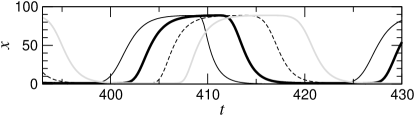
Figure 2: Propagation of a single kink around a ring of four elements with one inverter and $\tau=2$. The thick, thin, dashed, and grey lines represent element 1, 2, 3, and 0, respectively. Note that propagation is faster when the kink is positive and slower after the inverter converts it to a negative kink.

Until now, we have neglected the fact that the propagation speed of a kink through a given element is influenced by kinks that have previously passed through. Consider now an on pulse consisting of a positive kink followed by a negative kink. From Eq. (7), we see that $x_{j}(t)$ has an exponentially decaying memory of the events in $x_{j-1}(t)$. Because $f_{j}(x)$ is monotonic, the memory of low values of $x_{j-1}(t)$ before the pulse in $x_{j-1}(t)$ will speed up the effect of the trailing edge. The interaction shortens the pulse duration at $x_{j}(t)$, and monotonicity of $f_{j}$ ensures that the effect is stronger for shorter pulses. Similar reasoning shows that an off pulse will also be shorter than the time between kinks one would predict from Eq. (8) alone.

In a chain of copiers, different propagation speeds of positive and negative kinks will lengthen (shorten) a traveling on (off) pulse. In a chain that contains inverters arranged such that a single pulse spends equal amounts of time in its on and off configurations, the asymmetry between positive and negative kinks alone may not change the average pulse duration, but the pulse would still be shortened by the memory effect.

Because the strength of the memory effect increases as two kinks approach each other, a pulse or other sequence of kinks cannot propagate stably on a chain of single-input elements — only a single kink can have a stable shape as it advances. For simple rings, then, stable attractors must have only zero or one kink. These two possibilities correspond precisely to the fixed points and single-kink cycles that are the reliable attractors of the corresponding Boolean systems.

For rings with a self-input (Fig. 1), the situation is more complicated. First, note that the analysis of pulse propagation gives a quantitative measure of the asymmetry discussed above. The asymmetry enables some attractors classified as unreliable by the (symmetric) Boolean analysis to be stable in the continuous system. Second, memory effects associated with multiple inputs to a single element can lead to repulsion between pulses and stabilization of new attractors related to synchronous Boolean ones but with shifts in the timing between pulses.

IV Numerical results

We studied the three cases numerically using an integration scheme that takes advantage of the structure of Eq. (7) as described in Appendix B. In Case I, most initial conditions lead first to a long transient that corresponds to the unreliable attractor observed in the synchronous Boolean network. The transient eventually gives way to a stable attractor of Fig. 3(a), which has two pulses separated in time by approximately $(5/2)(\tau+1)$, an example of the stabilization of an intermediate inter-pulse interval where the synchronous Boolean attractor has pulses separated in time by alternating intervals of $2$ and $3$ time steps. We note in passing that the path by which the continuous system arrives at the attractor is rather robust: for a wide range of initial conditions, the system goes to the Boolean-like transient in a short time and then gradually shifts to the attractor. In some cases, however, we observe the attractor shown in Fig. 3(b), which has three pulses with a time separation of $(5/3)(\tau+1)$ between each pair. This attractor corresponds to a marginally stable cycle of the autonomous Boolean network, but the timing is incompatible with the synchronous updating scheme.

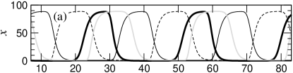
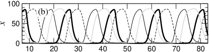
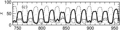
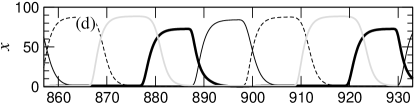
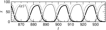
Figure 3: Time series for Cases I (a and b), II (c), and III (d and e), with $\tau=10$. The thick, thin, dashed, and grey lines represent element 1, 2, 3, and 0, respectively. Case I shows (a) non-synchronous timing stabilization due to memory effects (with time axis labels shifted by $10^{6}$ to account for a long transient) and (b) a stable attractor that has no analogue in the corresponding synchronous Boolean network. Case II shows (c) an inherently non-Boolean attractor. Case III shows (d) single pulse and (e) double pulse attractors, both of which are unreliable in a Boolean network.

We note that the appearance of attractor periods having $5(\tau+1)$ as an integer multiple can be understood analytically. Kaufman and Drossel have analyzed the possible attractor periods in synchronous Boolean networks in rings with a single cross-link Kaufman and Drossel (2005). A straightforward extension of their method to the autonomous networks of our ring with a nor self-input (Case I) reveals that all cycles in the autonomous model must have a period of the form $5/m$, where $m$ is an integer and the time unit is the time required for a kink to advance through one element. The corresponding period in the continuous model is therefore $5(\tau+1)/m$.

In Case II, two attractors are observed: the fixed point and an oscillatory attractor that appears to be aperiodic. The latter behavior is sensitive to intermediate variable values and is thus inherently non-Boolean. In Case III, we observe one fixed point and two limit cycles, corresponding to each of the three Boolean attractors, with no long transients. The limit cycles are unreliable in the Boolean case but stable in the continuous case — examples of stabilization due to asymmetry in kink propagation speeds and a pulse-shortening self-input element. This is the effect alluded to above at the end of the Boolean systems section. Though the pulse has broadened in traveling around the ring, a new trailing edge is generated by the self-input, which occurs one delay time after the arrival of the leading edge.

The difference in pulse height in the two limit cycles is due to the dependence of $f_{1}(x_{0},x_{1})$ on small variations in $x_{1}$ when $x_{0}$ is nominally on and $x_{1}$ is nominally off. The variations in the off-state of $x_{1}$ are caused by the delayed self-input that suppresses the off-state during a time of approximately $\tau$ following each pulse. In the limit cycle with two pulses, the suppression is still active when the next pulse starts. This is not the case for the single-pulse attractor and the slightly higher off-state leads to a suppression of the pulse height.

The above observations remain valid for all sufficiently large values of $\tau$. For small $\tau$, the systems studied have only fixed point attractors. As $\tau$ is increased, the oscillatory attractors are born by means of saddle-node bifurcations of cycles Strogatz (2000) in Cases II and III. In Case I, a subcritical bifurcation to a state cycle with period near $3\times(5/2)(\tau+1)$ is followed by a subcritical, symmetry-restoring bifurcation with period near $(5/2)(\tau+1)$. The cycle with period near $3\times(5/2)(\tau+1)$ has no direct correspondence to a cycle in the autonomous Boolean network.

V Discussion

Our study of simple and single-self-input rings has elucidated some important non-Boolean features of continuous systems: (i) the asymmetry in the reaction time of an element when an input switches on or off; (ii) deviations from nominal on and off values; and (iii) memory effects due to the exponential decay of variables to their steady state values for fixed inputs. These features are crucial for the stabilization and destabilization of oscillations in the systems we have investigated. In simple rings, they lead to a set of stable attractors that coincides precisely with the reliable attractors identified by Klemm and Bornholdt Klemm and Bornholdt (2005a). When more complex logic is introduced, as illustrated in here by adding a self-input to one element in a ring, the stable continuous attractors do not correspond to the reliable attractors.

These observations are important for generalizing the well-developed theory of large random Boolean networks to generic systems. We would like to know, for example, whether large, complex networks exhibit a well-defined dynamical phase transition similar to the “order-chaos” transition in ensembles of Boolean networks Kauffman (1969); Derrida and Pomeau (1986); Samuelsson and Socolar (2006). An important feature of the Boolean network transition is the rapid scaling of the number of attractors with system size in the disordered regime, which suggests that we should try to understand the set of attractors of large and complex continuous systems.

The non-Boolean effects discussed in this paper may also be directly relevant for understanding cell cycle oscillations in yeast, where there is evidence for a transcriptional oscillator and recent proposals for the genes involved suggest a fundamental ring of four elements with multiple feed-forward and feedback links Pramila et al. (2006). We have seen, for example, that a pulse of activity may propagate stably in such networks even where Boolean reasoning suggests otherwise. In systems where distinct elements have significantly different time delays, we expect additional deviations from the dynamics in synchronous or autonomous Boolean networks. Future studies along these lines should elucidate the behavior of larger rings and more complex network structures.

Appendix A Autonomous dynamics

For completeness, we describe the implementation of autonomous Boolean systems introduced by Klemm and Bornholdt Klemm and Bornholdt (2005a). The important features are that switching times are determined by local time delays and that repeated switching on times scales much shorter than the delay time is suppressed. There is no external clock and no stochastic rule for determining update times.

As in Ref. Klemm and Bornholdt (2005a), we assume a time delay of $1$ unit between the switching of a given node and the switching it induces in nodes directly linked to it. At each node, a low-pass filter is assumed to suppress spikes of duration much shorter than $1$. We let $\epsilon$ be the minimum duration of an output pulse that passes the filter (and require $0<\epsilon\ll 1$). If the inputs to a given node switch at times that would lead to a pulse shorter than $\epsilon$, the output from that node is assumed to stay constant during that time.

For notational convenience, we write $F_{j}(t)$, suppressing its direct dependence on its inputs. We also let the Boolean values off and on, respectively, correspond to the real values $0$ and $1$. Then, $x_{j}(t)$ is given by

$$x_{j}(t) =\Theta\biggl{[}\frac{1}{2\epsilon}\int_{-\epsilon}^{\epsilon}d\delta\left(F_{j}(t-1+\delta)-\frac{1}{2}\right)\biggr{]}\,,$$ (9)

where $\Theta(x)$ is the Heaviside step function; $\Theta(x)=0$ for $x<0$ and $1$ for $x\geq 0$.

When the timing of some switching events are perturbed infinitesimally, $F_{j}$ may switch twice in rapid succession, which would generate a positive or negative pulse of infinitesimal duration. The filter of Eq. (9) suppresses such spikes, ensuring that the number of switching events remains constant (for cycles in which all spikes are longer than $\epsilon$ in duration) and therefore that the stability of a state cycle is well defined with respect to infinitesimal timing perturbations.

Appendix B Numerical integration method

Numerical integration of the time-delay equations (1)–(4) was accomplished using a fourth-order scheme based on the solution shown in Eq. (7). To evolve the system through a time step $h$, we define values of $x$ at the time points $t=nh$ for all integer $n$ and define $m\equiv\tau/h$, where $\tau$ is the delay time and $h$ is chosen such that $m$ is an integer. To advance from time step $n-1$ to $n$ we use the following formula (suppressing the element index subscript $j$ for notational simplicity):

$$x_{n} =2h\left(\frac{1}{6}f_{n-m}+\frac{2}{3}e^{-h}f_{n-m-1}+\frac{1}{6}e^{-2h}f_{n-m-2}\right)$$

$$\phantom{=}~{}+\,e^{-2h}x_{n-2}\,,$$ (10)

where $f_{n}$ is the function defined by Eq. (2) [or (4)] evaluated at time $t=nh$. The integrator is initialized with a desired value of $x_{0}$, where it is assumed that $x_{n}=x_{0}$ for all $n<0$. Integrations were carried out using $h=0.1$. Decreasing $h$ to $0.01$ had no noticeable effect on the results.

Attractors were found by running from many (of order 50) different initial conditions. In some cases, such as the attractor shown in Fig. 3(b), it was necessary to arrange initial conditions in which some nodes were artificially held at constant values and released at different times. The bifurcation structures as a function of the time-delay parameter $\tau$ were determined by performing integrations in which $h$ was increased or decreased very slowly and observing transitions in the oscillation patterns of all $x$’s.

References

- Davidson (2006) E. H. Davidson, The regulatory genome: gene regulatory networks in development and evolution (Academic Press, 2006).
- Aldana-Gonzalez et al. (2003) M. Aldana-Gonzalez, S. Coppersmith, and L. P. Kadanoff, Boolean Dynamics with Random Couplings in Perspectives and Problems in Nonlinear Science, edited by E. Kaplan, J. E. Marsden and K. R. Sreenivasan (Springer, New York, 2003), p. 23.
- Aldana and Cluzel (2003) M. Aldana and P. Cluzel, Proc. Natl. Acad. Sci. USA 100, 8710 (2003).
- Greil and Drossel (2005) F. Greil and B. Drossel, Phys. Rev. Lett. 95, 048701 (2005).
- Moreira and Amaral (2005) A. A. Moreira and L. A. N. Amaral, Phys. Rev. Lett. 94, 218702 (2005).
- Kesseli et al. (2006) J. Kesseli, P. Rämö, and O. Yli-Harja, Phys. Rev. E 74, 046104 (2006).
- Paul et al. (2006) U. Paul, V. Kaufman, and B. Drossel, Phys. Rev. E 73, 026118 (2006).
- Samuelsson and Socolar (2006) B. Samuelsson and J. E. S. Socolar, Phys. Rev. E 74, 036113 (2006).
- Andrecut and Kauffman (2006) M. Andrecut and S. A. Kauffman, New J. Phys. 8, 148 (2006).
- Klemm and Bornholdt (2005a) K. Klemm and S. Bornholdt, Phys. Rev. E 72, 055101(R) (2005a).
- Flyvbjerg and Kjær (1988) H. Flyvbjerg and N. J. Kjær, J. Phys. A: Math. Gen. 21, 1695 (1988).
- Klemm and Bornholdt (2005b) K. Klemm and S. Bornholdt, Proc. Natl. Acad. Sci. USA 102, 18414 (2005b).
- Elowitz and Leibler (2000) M. B. Elowitz and S. Leibler, Nature 403, 335 (2000).
- Glass et al. (2005) L. Glass, T. J. Perkins, J. Mason, H. T. Siegelmann, and R. Edwards, J. Stat. Phys. 121, 969 (2005).
- Kaufman and Drossel (2005) V. Kaufman and B. Drossel, Eur. Phys. J. B 43, 115 (2005).
- Strogatz (2000) S. H. Strogatz, Nonlinear Dynamics and Chaos: With Applications to Physics, Biology, Chemistry, and Engineering (Westview Press, 2000).
- Kauffman (1969) S. A. Kauffman, J. Theor. Biol. 22, 437 (1969).
- Derrida and Pomeau (1986) B. Derrida and Y. Pomeau, Europhys. Lett. 1, 45 (1986).
- Pramila et al. (2006) T. Pramila, W. Wu, S. Miles, W. S. Noble, and L. L. Breeden, Genes & Dev. 20, 2266 (2006).