Many Attractors, Long Chaotic Transients, and Failure in Small-World Networks of Excitable Neurons

Abstract

We study the dynamical states that emerge in a small-world network of recurrently coupled excitable neurons through both numerical and analytical methods. These dynamics depend in large part on the fraction of long-range connections or ‘short-cuts’ and the delay in the neuronal interactions. Persistent activity arises for a small fraction of ‘short-cuts’, while a transition to failure occurs at a critical value of the ‘short-cut’ density. The persistent activity consists of multi-stable periodic attractors, the number of which is at least on the order of the number of neurons in the network. For long enough delays, network activity at high ‘short-cut’ densities is shown to exhibit exceedingly long chaotic transients whose failure-times averaged over many network configurations follow a stretched exponential. We show how this functional form arises in the ensemble-averaged activity if each network realization has a characteristic failure-time which is exponentially distributed.

Many systems in nature can be described as a network of interconnected nodes. A growing list of examples, from social and ecological webs to the neural anatomy of simple organisms, have been shown to exhibit complex topological features in stark contrast to ordered lattices or purely random networks. It is futhermore becoming increasingly clear that the details of the network architecture can crucially influence the emergent dynamics in the system. An understanding of the dynamics on complex networks requires investigation into the interplay between the instrinsic dynamics of the elements at the nodes and the topology of the network in which they are embedded. Here we study the collective behavior of excitable model neurons in a network with Small-world topology. The Small-world network is locally ordered but includes a certain number of randomly placed, potentially long-range connections which may act as short cuts. Such a topology bears a schematic resemblence to that found in the cerebral cortex, in which neurons are most strongly coupled to nearby cells, but are known to make long-range projections to cells millimeters away. We show that in the regime of low ‘short-cut’ density, persistent activity arises in the form of propagating excitable waves which annihilate upon meeting and are spawned anew via re-injection by long-range connections. A critical value of the ‘short-cut’ density at which network activity fails can be found by matching the longest distance on the network, a topological measure, to an intrinsic recovery time of the individual cells. We furthermore show how activity once again emerges at high ‘short-cut’ densities if the delay in the neuronal interactions is sufficiently long. The activity in this regime exhibits long, chaotic transients composed of noisy, large-amplitude population bursts. In this regime we investigate the interplay of the delay and the network topology numerically and provide a simple argument which provides a qualitative description of the distribution of failure times of the chaotic network activity.

I Introduction

It has been widely recognized that the connectivity of a network of active elements has a profound impact on its function. Substantial effort has therefore been devoted to the characterization of the network connectivity Albert and Barabasi (2002); Newman (2003) leading to the identification of various measures that are significant in determining the properties of the system. Particularly relevant among them are the average and maximal length of paths connecting arbitrary nodes in the network and the distribution for the number of links (degree) that emanate from the nodes.

The dynamics of networked elements has been studied in particular detail for coupled oscillators, addressing the influence of the network topology on their ability to synchronize. The existence of long-range connections between oscillators, which reduces the effective size of the network, has been found to enhance synchronizability substantially Barahona and Pecora (2002). At the same time, the heterogeneity of the degree distribution of many such networks limits the ability of the oscillators to synchronize, requiring a balance between the two aspects Nishikawa et al. (2003).

Excitable elements constitute a second important class of dynamical systems. In locally coupled networks they give rise to traveling waves (e.g. Bressloff (2000, 2001); Golomb and Ermentrout (2001)). If these waves annihilate upon mutual collisions, which is typically the case, persistent activity usually requires an external drive or spontaneous excitation by noise. In models for neural systems driven by noise Traub et al. (1999); Lewis and Rinzel (2000, 2001) networks with non-local connections between their elements have been shown to possess the tendency to exhibit relatively ordered oscillations in the population (mean) activity. The spatial structure of such noise-induced waves becomes less coherent with an increase in the non-local coupling Perc (2005). Combining local connectivity with a small number of non-local connections allows a localized time-periodic external input to entrain the whole system much faster than in a purely local network and at the same time the oscillations are much more coherent than in a truly random network Lago-Fernández et al. (2000, 2001). The dynamics depend very strongly on the duration of the refractory period relative to the propagation time scales and the range of the coupling. Thus, for very short refractory periods the small loops that are sufficiently likely in many types of random networks allow persistent activity even in the absence of noise as long as the initial conditions are asymmetric enough Carvunis et al. (2006). In an epidemic model the introduction of non-local connections was found to induce a transition to a state with coherent population oscillations Kuperman and Abramson (2001).

In most studies the connections between the elements have been assumed to be bi-directional, which is a very natural assumption in an epidemic context Kuperman and Abramson (2001) and can be for neural systems if the neurons are coupled via gap junctions Lewis and Rinzel (2000). In the absence of noise persistent activity is then only obtained with initial conditions that suitably break the reflection symmetry. If in an initially quiescent network individual neurons are excited by an external perturbation the pair-wise excited symmetrical waves are, however, all eventually annnihilated in collisions.

In neural systems the coupling between neurons is predominantly not bi-directional; instead most connections are via chemical synapses in which usually the information is only transmitted from the pre-synaptic axon to the post-synaptic dendrite. For these situations it is appropriate to consider directed networks with uni-directional connections. In previous work Roxin et al. (2004) we have investigated networks in which the local connections are bi-directional assuming that due to the close phyiscal proximity the probability for reciprocal axo-dendritic connections is quite high, but the non-local connections (‘short-cuts’) are uni-directional. Considering this directed modification of the by now classical small-world network Watts and Strogatz (1998), we found that even a few such uni-directional short-cuts allow for persistent activity even for generic localized excitations. As the density of short-cuts is increased, however, more and more network configurations support only a brief population burst after which the activity dies out. For slow propagation speeds of the waves the failure of network activity was found to be delayed and could occur after many cycles of chaotic population bursts. The simplicity of this model allowed an analytical result for the failure transition and detailed numerical analysis.

The results for the minimal system Roxin et al. (2004) provided important insight into the phenomena found in simlations of more elaborate models that were motivated by concrete biological situations. In Netoff et al. (2004) the connection between the topology of a neural network and its tendency towards epileptic seizures has been studied and related to the degree of recurrent connectivity of different parts of hippocampus. The origin of bursting behavior was addressed in Shao et al. (2006). Quite commonly bursting behavior arises when fast spiking behavior drives a slow process that in turn can shut off the spiking. Typically the slow process is associated with some slow kinetics. In Shao et al. (2006) the authors show that no such slow kinetics are needed in networks with small-world topology. Both the seizing and the bursting activity can be interpeted quite well based on an understanding of the failure transition in the basic model of Roxin et al. (2004). The rapid spread of activity and the persistent oscillations have also been observed in recent experiments on the Belousov-Zhabotinsky reaction in which the uni-directional short-cuts were implemented exploiting the photo-sensitivity of the reaction Tinsley et al. (2005); Steele et al. (2006).

Here we build on our previous results and present a detailed characterization of the persistent states and the dependence of their properties on the prevalence of short-cuts as well as of the long chaotic transients for which we provide an understanding of the stretched exponential behavior in their failure times. In Section II we define the model, which consists of ‘Integrate-and-Fire’ neurons that are coupled via excitatory pulses in a small-world topology with uni-directional short-cuts. In Section III we discuss in detail the persistent states and the cross-over from persistent activity to failure for the case of rapidly propagating waves. In Section IV we provide a detailed analysis of the exceedingly long chaotic transients in the regime of slower propagation. In the concluding Section V we discuss our results in light of other work on neural networks with small-world topology Netoff et al. (2004); Shao et al. (2006).

II Neuron Model and Network Topology

We consider a one-dimensional network of $N$ identical integrate-and-fire neurons. Their membrane voltage is described by

$$\tau\frac{dV_{i}}{dt} = -V_{i}+RI_{ext}+g_{syn}\sum_{j=1}^{N}w_{ij}\delta(t-t^{j}-\tau_{D}),$$ (1)

with the reset condition

$$V(t^{+}) = V_{res}\hskip 36.135pt\textrm{whenever}\hskip 36.135ptV(t^{-})=V_{th},$$ (2)

Here $\tau$ is the membrane time constant, $g_{syn}$ is the synaptic strength measuring the change in voltage due to one incoming action potential, $w_{ij}=0$ or $1$ indicates the absence or presence respectively of a synaptic connection from neuron $j$ to neuron $i$, $t^{j}$ is the time at which neuron $j$ fires an action potential, $I_{ext}$ is an external current and $R$ the membrane resistance. The effective delay $\tau_{D}$ in the neuronal interaction includes the time for the signal to propagate along the axon as well as the time needed for initiating the triggered action potential. If the latter time dominates over the axonal delay the dependence of the delay on the distance between the neurons involved can be neglected. Post-synaptic currents due to synaptic activation are considered instantaneous and are therefore modeled as Dirac-delta functions. Eq.(2) reflects the fact that whenever the voltage of neuron $i$ reaches the threshold value $V_{th}$, a spike is emitted and the voltage is reset to the value $V_{res}$. We write Eq.1 in terms of dimensionless quantities by setting without loss of generality $V_{res}=0$, rescaling $V$ and $g_{syn}$ by $V_{res}$ and time by $\tau$ , and by replacing $I_{ext}$ by the steady-state voltage $V_{\infty}$, to which it corresponds in the absence of synaptic input. We focus on the case of excitable rather than spontaneously oscillating neurons, i.e. $V_{\infty}<1$, and consider only initial conditions in which at most a few neurons are triggered to spike with all other neurons quiescent. In the absence of noise this implies that neurons can only fire at times that are multiples of $\tau_{D}$ and the model can be solved exactly between these times. In the numerical computations the time step is therefore taken to be $\Delta t=\tau_{D}$.

In cortex neurons receive often not only local input from neurons near-by but also input from some distant neurons through long-range projections. We mimic such a heterogeneous connectivity with an extremely simplified architecture for the network in which each neuron is connected to $2k$ neighbors, i.e. $w_{ij}=1$ for $j\leq i\pm k$ and $j\neq i$ and an additional $pN$ neurons that are chosen randomly. The parameter $p$ thus gives the density of random uni-directional connections as a fraction of the total number of neurons $N$.

The dynamics arising in Eqs(1,2) for purely local connectivity ($p=0$) depend, in the absence of noise, on the interplay between the strength of the synapses $g_{syn}$, the number of neighbors $2k$, and the delay $\tau_{D}$. This is most easily illustrated for nearest-neighbor connectivity ($k=1$). In this case, if $g_{syn}+V_{\infty}<1$ the pre-synaptic input is insufficient to cause a spike and no network activity will occur. For stronger input, i.e. for $g_{syn}+V_{\infty}>1$, a wave of speed $1/\tau_{D}$ is generated. After the spike the voltage is reset to $V=0$ and the neuron is only ready to fire again after it has recovered to the extent that an input of magnitude $g_{syn}$ is sufficient to trigger another spike. This recovery time is given by

$$T_{R}=\ln{\Bigg{(}\frac{V_{\infty}}{V_{\infty}+g_{syn}-1}\Bigg{)}}$$ (3)

Note, that $T_{R}$ is not an intrinsic refractory period of the neuron since for sufficiently strong input $g_{syn}$ this model neuron can fire arbitrarily fast.

Due to the bidirectionality of the local connections the firing of each neuron not only triggers a spike in the neuron ahead of it in the wave of excitation, but gives also an input to the neuron behind it. Thus, the latter neuron receives already a first input at a time $2\tau_{D}$ after its firing. If $T_{R}>2\tau_{D}$ this input is not sufficient to trigger a spike and the activity propagates away from the site of initiation as each neuron contributes exactly one spike, see Fig.1a. If, however, $T_{R}\leq 2\tau_{D}$ then the wave front entrains all the neurons in its wake, eventually leading to synchronized activity of the whole network. Unless autapses with $w_{ii}\neq 0$ are included the network breaks up into two synchronous groups of neurons that fire out of phase with one another, see Fig.1b. In the general case, a propagating wave can be sustained if $g_{syn}e^{\tau_{D}}\sum_{n=1}^{k}e^{-n\tau_{D}}+V_{\infty}>1$. That is, a neuron receives inputs from $k$ neighbors as the wave approaches, with an input at a distance $n$ discounted by $e^{(1-n)\tau_{D}}$. For simplicity we will focus on the case of nearest-neighbor coupling ($k=1$) , and will consider the regime in which waves of excitation propagate, but do not entrain activity in their wake. This choice constrains the allowable values of $V_{\infty}$ and $g_{syn}$. Specifically, we take $V_{\infty}=0.85$ and $g_{syn}=0.2$ unless otherwise noted. In this regime the collision of two waves leads to their mutual annihilation and after having fired in a propagating wave a neuron can be re-excited by a single input of size $g_{syn}$ after a time

$$T_{R}^{(1)}=\ln{\Bigg{(}\frac{V_{\infty}-g_{syn}e^{2\tau_{D}}}{V_{\infty}+g_{syn}-1}\Bigg{)}}.$$ (4)

This time includes the input after a delay of $2\,\tau_{D}$ from the neuron further ahead in the wave.

Figure 1: Dynamics in the flocal network of 50 neurons with nearest-neighbor coupling. Parameters are $V_{\infty}=0.85$ and $\tau_{D}=0.1$. (a) $g_{syn}=0.2$: An example of a propagating wave. The wave fronts meet and annihilate at time 2.5. Top: Raster plot showing the times at which the neurons fire an action potential. Middle: The averaged firing rate of the network. Bottom: The voltage of neuron number 20. (b) $g_{syn}=1.0$: The wave entrains all the neurons in its path. The final state of the network is one in which two synchronous groups of neurons fire out of phase with one another. Note: The maximum possible firing rate is $1/\tau_{D}=10$.

Eqs(1,2) with the above-mentioned assumptions are a minimal model for the generation and propagation of waves in cortical-like tissue. As we shall see, the addition of random, long-range connections qualitatively alters the dynamics of the network, allowing for a rich variety of spatio-temporal patterns.

III The ordered regime: Attractors and Failure

Once the input current $V_{\infty}$ and synaptic strength $g_{syn}$ have been fixed, the dynamics arising in Eqns(1) and (2) are determined by the remaining two parameters: the fraction of randomly placed connections $p$ and the delay in the neuronal interaction $\tau_{D}$.

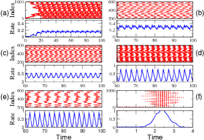
Figure 2: Examples of the network dynamics as a function of the density of short-cuts $p$. Here $p=0.01,0.05,0.1,0.15,0.2,0.25$ for (a) through (f) respectively. $\tau_{D}=0.1$.

The dynamics for non-vanishing $p$ differ qualitatively from those without any long-range connections. The presence of long-range connections (‘short-cuts’) allows the waves of excitation to be re-injected into portions of the network which have already been excited. This process of re-injection may lead to persistent network activity as shown in Fig.2. As the waves spread outward from the initial site of stimulation they encounter long-range connections and are injected elsewhere in the network. Wavefronts that meet annihilate. After some time, the activity settles into a stable pattern in which the rates of generation and annihilation of the waves balance. Averaged over time and across configurations, the firing rate of these persistent states increases rapidly with increasing number of short-cuts and saturates around $p\sim 0.1$ (Fig.3). This saturation is a consequence of the neuron’s finite recovery period $T_{R}^{(1)}$ given in Eq.4. The bars in Fig.3 give the standard deviation of the firing rate across configurations for $\tau_{D}=0.1$. Clearly in some configurations the firing rate comes very close to its maximal value. As the system size is increased this saturation level is reached already for smaller values of $p$ (Fig.3b).

The firing rate is essentially the inverse of the time between successive waves passing through a given point. Thus, one may expect that decreasing the wave speed by increasing $\tau_{D}$ would reduce the mean firing rate. This is, however, not the case; instead the firing rate is quite insensitive to the wave speed as shown in Fig.3b. The reason for this is apparent in Fig.4a,b. It shows two simulations for the same network configuration but with different delay times $\tau_{D}$. For larger delay $\tau_{D}$ additional waves are excited by the short-cuts as can be seen, for instance, at $t=380\tau_{D}$ where a new wave can be spawned at neuron 1071 for $\tau_{D}=0.1$ but not for $\tau_{D}=0.05$ (marked by circles). This increases the firing rate, and in the case shown it even over-compensates the reduced wave speed, as can be seen by the higher density of waves for $\tau_{D}=0.1$ at larger times.

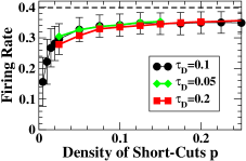
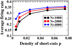
Figure 3: The firing rate is close to $1/T_{R}^{(1)}$. The firing rate averaged over 1000 configurations (5,000 for $p>0.2$) as a function of the density of shortcuts $p$ for different values of the delay $\tau_{D}$ ($N=1000$) (a) and for different values of the system size $N$ ($\tau_{D}=0.1$) (b). The theoretical maximal valueof $1/T_{R}^{(1)}$ is indicated by the dashed line. The bars indicate twice the standard deviation across configurations.

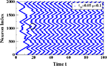
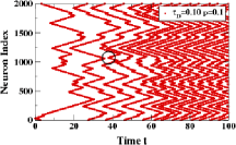
Figure 4: For longer delay in an identical network, more waves can travel through the system. Raster plots for $\tau_{D}=0.05$ and $\tau_{D}=0.1$ with $p=0.1$ and $N=2000$. Circles mark where a new wave is spawned for $\tau_{D}=0.1$ but not for $\tau_{D}=0.05$.

For low $p$ only a few short-cuts are present and many pathways leading to persistent activity consist only of large closed loops, implying low firing rates. As $p$ increases the typical loop sizes decrease and network configurations with large minimal loops and correspondingly low firing rates become increasingly unlikely. This is seen in the distribution function for the firing rate shown in Fig.5. As the distribution function is shifted towards larger firing rates with increasing $p$ it narrows substantially reflecting the maximal firing rate set by the recovery time $T_{R}^{(1)}$, which is marked by a dashed line in Fig.5.

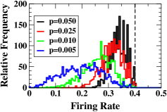
Figure 5: Distribution of firing rates across configurations for various values of $p$. As $p$ increases the distributions narrow in width and approach the value $1/T_{R}^{(1)}$ (dashed line). $N=2,000$, $\tau_{D}=0.1$

The activity into which the network eventually settles is periodic in time and with increasing number of short-cuts the amplitude of the oscillations increases. This is shown quantitatively in Fig.6, which characterizes the magnitude of the oscillations by the standard deviation of the firing rate averaged over a large number of persistent configurations. As is apparent from Fig.2, the time for these oscillations to establish themselves from the excitation of a single neuron decreases with increasing $p$. This corresponds to the main result of Lago-Fernández et al. (2000, 2001) where it was found that in the small-world regime a network of Hodgkin-Huxley neurons and of FitzHugh-Nagumo neurons is entrained much more quickly by a cluster of driven, oscillating neurons.

Figure 6: Oscillation amplitude increases with the number of short-cuts. Dependence of the standard deviation of the firing rate (for persisting activities) averaged over up to 5,000 configurations for $\tau_{D}=0.1$. $N=1000$.

For larger values of $p$ the activity patterns can be quite complicated. While in this regime all neurons get excited during an oscillation cycle, not all neurons and connections between them are necessary for the persistence of the activity. This is illustrated in Fig.7. The full raster plot is depicted in the top panel (black dots). Superimposed on it are those neurons that are essential for carrying on the activity; they constitute the pathway of this activity Roxin (2003). It is is determined as follows. Once the simulation has been run, all the neurons that fire at the final time are labeled. For each of the labeled neurons, a search is carried out for presynaptic active neurons, i.e. neurons that fired one delay $\tau_{D}$ ago and triggered the currently firing neurons. These ‘causal’ presynaptic neurons are labeled in turn. This process is carried on backwards in time until $t=0$. The pattern of labeled neurons quickly converges to a small subset, see middle panel of Fig.7. Only the neurons in this much simpler subset contribute to the persistence of the pattern, i.e. the remaining neurons could be cut out of the network without destroying the persistent activity. In Fig.7, the pathway of activity (shown blown up in the bottom panel) is periodic in time with a period that is only slightly longer than the recover time $T_{R}^{(1)}$, indicated by the dashed lines. Such pathways have also been identified in an experimental study of the photo-sensitive, excitable Belousov-Zhabotinsky reaction in which short-cuts were introduced through local optical excitation Steele et al. (2006).

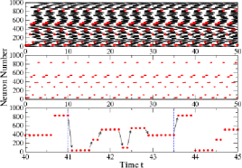
Figure 7: An example of a ’pathway’ of excitation. The pathway responsible for persistence is shown in red and is longer than the recovery time $T_{R}^{(1)}$, indicated by the dashed lines in the lower panel. $\tau_{D}=0.1$ and $p=0.1$. See text for details.

A striking feature of this regime is the fact that for a given network configuration there is an extraordinarily large number of different attractors. To assess the degree of multiplicity of attractors we focus on the regime with low short-cut density where all solutions are periodic and characterize each solution by its period, its mean firing rate, and the standard deviation of the firing rate. Clearly, distinguishing different solutions by only these three measures may underestimate the total number of attractors. Fig.8 illustrates the attractor multiplicity for a single, randomly chosen network configuration of $N=1000$ neurons for $p=0.05$ and $\tau_{D}=0.1$. In Fig.8a presents each of the 471 different solutions that can be reached by exciting initially a single neuron with all other neurons being at rest. As shown more clearly in Fig.8b, which gives the number of initial conditions that lead to a solution with a given period (irrespective of their firing rate and its standard deviation), only few values for the period arise (note the logarithmic scale). In contrast, the standard deviation of the firing rate (Fig.8c) can take on many different values, each representing a different temporal evolution of the firing during the period.

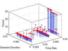
Figure 8: Large number of attractors. a) Mean firing rate, its standard deviation, and period of all 471 attractors obtained for a single configuration for $N=1000$, $p=0.05$, and $\tau_{D}=0.1$. b) Number of initial conditions leading to an attractor with a given period. Many attractors, although distinct, have the same period. (note logarithmic scale). c) Number of initial conditions leading to an attractor with a given standard deviation of the firing rate.

The large number of attractors is typical for these networks as seen in Fig.9, which presents the number of attractors as a function of the network size averaged over 20 different configurations (black circles). A large fraction of the attractors has a quite small basin of attraction: within the restricted set of initial conditions in which only a single neuron is excited, they are reached from only a single initial condition (red squres). The overall number of attractors seems to increase roughly linearly with system size for larger values of $N$, while the number of attractors with different periods (green diamonds) seems to grow more rapidly than that. Since the duration of the transients grows with system size the computation time grows faster than $N^{2}$. This precludes us from going to significantly larger system sizes than shown in Fig.9 , which would be necessary to get a reliable estimate for this scaling. Preliminary computations indicate that allowing more general initial conditions significantly increases the number of attractors beyond those shown in Fig.8. Thus, while the restricted initial conditions employed in Fig.9 suggest an almost linear increase in the number of attractors with system size, the full number of attractors may grow substantially faster. At this point the origin for the exceedingly large number of different attractors is not clear. In all-to-all coupled oscillator systems factorially large numbers of attractors have been found due to the permutation symmetry of that global coupling Wiesenfeld and Hadley (1989). The small-world networks investigated here do not possess any such symmetries.

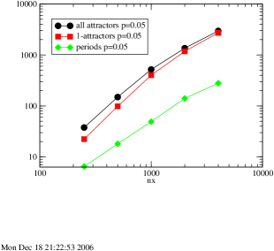
Figure 9: Dependence on the system size. All attractors (circles), attractors with basin of attraction 1 (squares), attractors with different period (diamonds).

As the value of $p$ increases, the distance traveled by the waves before encountering a long-range connection decreases. Consequently, the waves of excitation spread throughout the network more rapidly. This effect can be seen clearly in the progression of spatio-temporal patterns in Fig2(a-e). For sufficiently large values of $p$ the activity spreads too quickly to sustain the activity, see Fig.2f. Since the long-range connections are made randomly, the dynamics vary across network configurations. Thus, while the overall likelihood of persistent activity should decrease with increasing $p$, the actual network dynamics depend on the particular network configuration.

The dynamical mechanism leading to the extinction of network activity is easily elucidated Roxin et al. (2004). Once a neuron has emitted a spike, its voltage is reset, here to $0$. As the voltage of the neuron recovers to its resting potential, here equal to $V_{\infty}$, the activity spreads through the network, eventually finding its way back. Once this occurs, the neuron receives synaptic input equal to $g_{syn}$. This input will be only sufficient to trigger a spike in this neuron if the neuron has sufficiently recovered. It is therefore clear that the more rapidly the activity spreads, the less likely the network will be to exhibit persistence. Whether or not this mechanism leads to the extinction of activity in a given network depends on the particular network topology. For fixed $p$ many configurations of the network can be simulated to calculate the percentage of network configurations for which the activity is extinguished, as shown in the left inset of Fig.10. In agreement with our intuitive argument, the likelihood of the activity failing for a particular configuration drawn at random increases with increasing $p$. In fact, for large enough systems it seems that there is a transition or, more precisely, a cross-over from a regime in which all network configurations exhibit persistent activity, to one in which the activity will always fail. The transition moves to larger values of $p$ as the system size $N$ increases.

As discussed in Roxin et al. (2004), this transition can be captured in a mean-field approximation in which the return time is identical for all neurons. In this case the dependence on the long-range component of the topology can be expressed as a function of $p$ alone. Setting the maximum return time $T_{A}$ (the time needed for the activity to traverse the entire network) equal to the recovery time yields an upper bound for the density of long-range connections at which a transition from persistent activity to failure occurs

$$T_{A}(p_{cr})=T_{R}^{(1)}.$$ (5)

An approximate form for $T_{A}$ is easily derived. We assume that a single neuron fires at time $t=0$. Given a density $p$ of shortcuts, we expect a long-range connection will be reached after $1/p$ neurons have fired, which occurs after a time $\tau_{D}/2p$ since there are two wave fronts. Four wave fronts are now present and so $2/p$ neurons will fire in a time $\tau_{D}/2p$ at which point on average two new wave fronts are generated, and so on. During the $k^{th}$ cycle, the number of neurons excited is $2^{k-1}/p$. After $n$ cycles all the neurons have been excited, which results in

$$\sum_{k=0}^{n-1}2^{k}=pN$$ (6)

and leads to a time

$$T_{A}(p)\equiv n\frac{\tau_{D}}{2p}=\tau_{D}\frac{\ln{(1+pN)}}{2p\ln 2}.$$ (7)

Equation (7) is a purely geometric result, since the time it takes for activity to traverse the entire extent of the network is related trivially to the largest distance in the network. The geometric mean-field properties of small-world networks have been worked out by Newmann, Moore and Watts. In Newman et al. (2000) they calculate the fraction of a small-world network covered by starting at a single point and extending outwards a distance $r$ in both directions (equivalent to waves having spread for a time $r\tau_{D}$ in our case) in a continuum limit. In Newman et al. (2000) they refine the continuum limit calculation by taking into account two effects that were omitted from their earlier calculation Newman and Watts (1999) and from ours. Firstly, as they trace out the network, a jump via a long-range connection may reach a part of the network that has already been traced over and should therefore not be counted. We interpret this as activity spreading via long-range connections, which is injected into a neuron that has already fired but is not ready yet. Such a connection would therefore be ineffectual. Secondly, when two ‘traced-out’ sections meet, they stop and no longer contribute. We interpret this as wavefronts which meet and annihilate and thus, thereafter, do not contribute. Considering these two additional mechanisms, they develop a two-component model that describes, effectively, the fraction of the network covered and the number of fronts. The result, interpreted within the context of equation (1), yields,

$$\sqrt{\Big{(}1+\frac{4}{pN}\Big{)}}\tanh{\Big{[}\sqrt{\Big{(}1+\frac{4}{pN}\Big{)}}\frac{pT_{A}(p)}{2\tau_{D}}\Big{]}}=1.$$ (8)

Setting $T_{A}(p_{cr})=T_{R}^{(1)}$, yields the density $p_{cr}^{(MFT)}$ at the failure transition.

The main panel in Fig.10 shows the failure rates, rescaled by the critical density $p_{cr}^{(MFT)}$ calculated from Eq.(8). All failure curves intersect at the same value of $p$, which defines therefore the transition point $p_{cr}$. Consistent with the upper bound obtained in the mean field theory $p_{cr}<p_{cr}^{(MFT)}$. Unfortunately, we need to point out that the good quantitative agreement reported in Roxin et al. (2004) was spurious; there we incorrectly used $T_{R}$ instead of $T_{R}^{(1)}$ as the recovery time in (8) (cf. Fig.11). For comparison with the approximate mean field calculation the right inset shows the failure curves rescaled by $p_{cr}$ as obtained from (7).

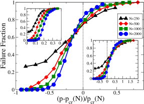
Figure 10: Failure Transition as a function of system size $N$. Fraction of failing configurations rescaled by $p_{cr}$ from Eq.8. Left inset: unscaled data. Right inset: data rescaled by $p_{cr}$ from Eq.7.

The central quantity determining the persistence or failure for a given short-cut configuration is the recovery time $T_{R}^{(1)}$. It is worth pointing out that this time is not the same as an absolute refractory period $T_{r}$ of the neuron. While $T_{r}$ is a property of the neuron independent of its neighbors, $T_{R}^{(1)}$ depends strongly on the strength of the coupling between the neurons. As long as the refractory period is shorter than the recovery time it has little effect on the persistence of the network. This is illustrated in Fig.11, which shows the fraction of persisting configurations for a network of neurons with an absolute refractory period $T_{r}$ during which they do not respond to any input from other neurons. During that time their membrane voltage $V$, however, still relaxes towards its resting value. For $T_{r}<2\tau_{D}$ the second input characteristic of propagating waves (cf. (4)) is unaffected and the relevant recovery time is $T_{R}^{(1)}$. The resulting failure curve ($T_{r}=0$) corresponds to those in Fig.10. For $2\tau_{D}<T_{r}$ the second input is suppressed. In this low-$p$ regime the persistent states do not depend on neurons receiving any further additional inputs before their firing (cf. Sec.IV) and the failure transition is independent of $T_{r}$ as long as $2\tau_{D}<T_{r}<T_{R}$. Only for $T_{r}>T_{R}$ does the transition depend on the absolute refractory period.

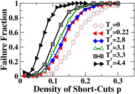
Figure 11: Dependence of failure on refractory period $T_{r}$ for $N=1000$, $\tau_{D}=0.1$ ($T_{R}=2.83$), and 500 configurations.

IV The disordered regime: chaotic transients for slow waves

For small values of $p$ we have seen that the likelihood of persistent activity is high. In this regime, the spatio-temporal activity, despite the complex, heterogeneous topology of the network itself, is highly regular and most often periodic. As $p$ increases a transition in the likelihood of persistent activity occurs and more and more network configurations exhibit activity which peaks and then shuts down. Interestingly, for large enough $\tau_{D}$ there is an additional change in the behavior of the network as $p$ increases, see Fig.12. Specifically, one finds that while the likelihood of failure initially increases for low $p$, as described in the previous section, it then turns downward again for larger values of $p$, see the curves for $\tau_{D}=0.16$ and $0.18$ in Fig.12. To understand why this is so, we first describe the spatio-temporal dynamics underlying this seemingly persistent activity.

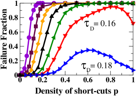
Figure 12: Failure curves for different values of the delay $\tau_{D}=0.06,0.08,0.1,0.12,0.14,0.16$. Each symbol is the average of 2000 configurations. For large enough delay, $\tau_{D}=0.16$ and $0.18$, the likelihood of failure before a finite time $T^{*}=100$ becomes non-monotonic in $p$.

Fig.13 shows four typical raster plots of the activity seen for $\tau_{D}=0.16$ as a function of $p$. For values of $p$ below or near the theoretical transition to failure (panels (a) through (c)), the activity is similar to that seen in Fig.2. In the regime beyond the maximum of the failure curve (panel (d)) the activity is chaotic (cf. Fig.14a below) and exhibits irregular population spikes reflecting near-synchronous activity involving a large fraction of the neurons.

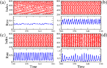
Figure 13: Raster plots and firing rate for four typical configurations for ’slow’ waves, $\tau_{D}=0.16$. $p=0.01,0.2,0.4$ and $1.0$ for (a) through (d) respectively. The activity in the ’high’ $p$ regime seen in (d) is unlike that seen in the other three. It is noisy and exhibits synchronized population spikes.

A more detailed, quantitative analysis for $\tau_{D}=0.18$ shows that the change in behavior occurs already before the maximum of the failure curve. For the fast waves (small $\tau_{D}$) the oscillation amplitude as measured by the standard deviation of the firing rate increases monotonically with $p$ (cf. Fig.6). For slower waves it is, however, non-monotonic and decreases over the range $0.4\leq p\leq 0.6$ (Fig.15 $\tau_{D}=0.18$). More instructive yet is the dependence of the spectral entropy of the firing rate,

$${\mathcal{E}}=-\sum_{\omega}S(\omega)\,\ln S(\omega),$$ (9)

which measures the number of significant peaks in the power spectrum ${\mathcal{S}}(\omega)$. Its average over 200 configurations rises significantly in this range of $p$, as shown in Fig. 15, indicating an increase in the complexity of the dynamics. The variability of ${\cal E}$ across the configurations exhibits a (broad) maximum in the transition region and reaches very small non-zero values around ${\mathcal{E}}\sim 0.06$ in the strongly chaotic regime. We have not investigated details of this evolution towards chaotic dynamics, which depends on the individual configurations of the short-cuts.

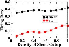
Figure 14: Oscillation amplitude depends non-monotonically on the density of short-cuts. Mean and standard deviation of the firing rate is shown for those configurations (out of 200) for which the activity persists for at least 15,000 steps. ($\tau_{D}=0.18$, $N=1000$).

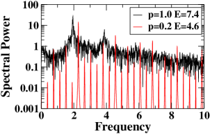
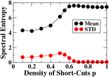
Figure 15: Temporal behavior becomes increasingly complex with increasing $p$. a) Representative power spectra for $p=0.2$ (${\mathcal{E}}=4.6$) and $p=1.0$ (${\mathcal{E}}=7.4$). b) Spectral entropy $S$ (mean and standard deviation across 200 configurations). ($\tau_{D}=0.18$, $N=1000$ and 15,000 time steps)

What causes the dynamics to re-emerge as $p$ increases? The answer lies in the interplay between network topology and the delay $\tau_{D}$. In order to develop the mean-field model, eq.(5) we assumed that the firing of each neuron is limited by the recovery time $T_{R}^{(1)}$. However, even for $p<1$ the construction of the network allows for some neurons to receive more than one incoming short-cut. For our network it can be shown Roxin (2003) that for $p$ small, the fraction of neurons with two incoming short-cuts is $s_{2}\sim p^{2}/2$, which is indeed negligible. Thus, the mean-field results should hold if the transition occurs at sufficiently low values of $p$. However, for $|p-1|\ll 1$ the fraction of neurons with two inputs becomes $s_{2}=1-\sqrt{2}/2+(p-1)/2$ which is nearly $0.3$ for $p=1$. Thus, a significant subpopulation of neurons likely receives several inputs per cycle. Such neurons would not be constrained by the recovery time $T_{R}^{(1)}$ but rather would be primed to fire earlier, potentially allowing the activity to persist where it otherwise would fail. We can easily calculate the recovery time for a neuron $i$ which, by virtue of several incoming connections, has received $n$ inputs since its last firing

$$T_{R}^{(n)}(t_{1},...,t_{n})=\ln{\Bigg{(}\frac{V_{\infty}-g_{syn}\sum_{r=1}^{n}e^{t_{r}}}{V_{\infty}+g_{syn}-1}\Bigg{)}}.$$ (10)

Note that Eq.(10) reduces to Eq.(3) for $n=0$ and to Eq.4 for $n=1$ with $t_{1}=2\tau_{D}$. In general, $T_{R}^{(n)}$ depends on the $n$ firing times of those neurons providing input to neuron $i$, which are unknown. However, since integrate-and-fire neurons become increasingly sensitive to their input as time passes after their firing, the value of $T_{R}(n)$ in Eq.(10) is bounded below by $T_{R,min}^{(n)}$, which occurs when all $n$ inputs coincide at $T_{R,min}^{(n)}$ itself. This time is given by

$$T_{R,min}^{(n)}(t_{i}=T_{R,min}^{(n)})=\ln{\Bigg{(}\frac{V_{\infty}}{V_{\infty}+ng_{syn}-1}\Bigg{)}},$$ (11)

For small enough $p$ the inter-spike intervals (ISI) of almost all the neurons are bounded below by $T_{R}^{(1)}$, which allows us to calculate the time for activity to spread throughout the whole network using a geometrical approach. For higher values of $p$ there may be a subset of neurons with shorter allowable ISI. However, many neurons will still only receive a single input per cycle and their activity should reflect this fact. This is borne out in the distribution function for the ISI shown in Fig.16. ‘Fast’ spikes with ${\rm ISI}<T_{r}^{(1)}$ occur appreciably only for $p\geq 0.6$ and increase further in frequency with increasing short-cut density. Our previous analysis Roxin et al. (2004) showed that the spikes with ${\rm ISI}>T_{R}^{(1)}$ occur in population bursts with no such spikes in between. In the absence of other spikes the activity would die out during these periods. However, due to the large number of short-cuts there is a substantial number of neurons that have received multiple inputs and are consequently primed to carry over the activity to the next cycle, thereby allowing the ‘slow’ spiking neurons to recover.

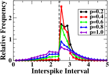
Figure 16: Distribution of interspike intervals (ISI) for $\tau_{D}=0.16$ and a range of $p$. For low $p$ all ISI are above the recovery period $T^{(1)}_{R}$ (dashed line). For $p\geq 0.6$ increasingly more multiple inputs allow shorter ISI.

Increasing the delay $\tau_{D}$ contributes in a number of ways towards bridging low-activity periods. For larger $\tau_{D}$ the failure transition is shifted towards larger short-cut densities enhancing the number of multiple-input neurons significantly. At the same time, in order to bridge the time between the relatively short return time $T_{A}$ and the recovery time $T_{R}^{(1)}$ of the slow neurons fewer fast neurons with multiple input are needed if the delay is longer. Moreover, for the integrate-and-fire neurons (1) later inputs have a stronger impact on the recovery period than earlier ones (cf. Eq.(10)). With increasing $\tau_{D}$ all inputs are shifted to later times relative to the last spike of the respective neuron, which reduces the recovery time significantly. The increased delay is, however, not necessary to reach the regime of prolonged activity. As shown in Fig.17 for fixed delay $\tau_{D}=1.4$, increasing the system size from $N=1,000$ to $N=16,000$ shifts the failure transition to sufficiently large $p$ that the number of neurons with multiple inputs is sufficient to bridge the gap in slow-neuron activity even for this lower delay time.

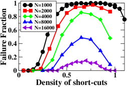
Figure 17: Prolonged activity in large systems. Failure rates up to a final time $T^{*}=28$ for $\tau_{D}=0.14$ (400 configurations).

For low values of $p$ the spatio-temporal dynamics are most often periodic. In those cases the dynamics can truly be called persistent. For $p\sim 1$, the chaotic nature of the dynamics precludes such a clear assessment and, in fact, failure is possible even after very long times. Since persistent activity relies on a bridging of the quiescent period by a string of neurons that have multiple incoming short-cuts it is necessary that these short-cuts are actually activated during the previous cycle and at suitable times. Thus, while in one cycle the activity during the burst may have been able to excite such a chain the different activity pattern in the next cycle may fail to do so and the activity could die out. Indeed, we find that for these large short-cut densities the activity eventually fails for essentially all configurations. Examples of such long-lived transients are shown in Fig.18, where firing rates are shown for the same configuration of short-cuts but increasing values of $\tau_{D}$. Clearly, the delay has a strong influence on the duration of the transient (note the change in scale on the $x$-axis).

Figure 18: The firing rate for four values of the delay $\tau_{D}$, with $p=1$. The network architecture and initial condition are identical for all four simulations, only the delay has been changed. Failure tends to occur at longer times for larger delays.

While overall there is a trend for the lifetimes of the transient activity to increase with increasing delay, the actual dependence on $\tau_{D}$ is more subtle. Fig.19 shows, as a function of $\tau_{D}$, the fraction of configurations for which the activity fails before the final time $T^{*}$ is reached. The dependence on $\tau_{D}$ exhibits an amazing degree of structure. Most surprising is the finding that an increase in $\tau_{D}$ does not always decrease the number of failures, but can in fact enhance the probability of failure. These changes can occur over very small intervals in $\tau_{D}$ as shown more clearly in Fig.19b. This fine structure is reminiscent of ‘resonances’ or ‘windows’ in which the delay is $\tau_{D}$ ‘optimal’. While details of the mechanism underlying this structure are not understood yet, it is clear that the dependence on $\tau_{D}$ reflects the significance of the ratio $\tau_{D}/T_{R}$. This is further illustrated in Fig.20 where the failure rates are shown for a reduced number of neurons, $N=500$. While the failure rates are higher overall in the smaller system, the locations of the windows in $\tau_{D}$ are not substantially altered. If however, the recovery time is reduced from $T_{R}=2.83$ to $T_{R}=2.79$ by increasing the synaptic strength from $g=0.2$ to $g=0.202$, the windows are clearly shifted to lower values of $\tau_{D}$.

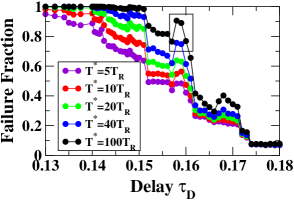
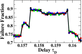
Figure 19: a) Failure rates for a range of final times $T^{*}=5T_{R}$, $10T_{R}$, $20T_{R}$, $40T_{R}$, $100T_{R}$ based on 2000 configurations with $p=1$ and $N=1,000$. The range covered in b) is marked by a box. b) Fine structure in the failure rate for $T^{*}=100T_{R}$ based on four runs with 8000 configurations each. Black line gives average over the 4 runs.

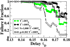
Figure 20: Failure rates based on 8000 configurations with $p=1$ for $N=500$ for $g=0.2$ and $g=0.202$. For comparison also the case $N=1000$ is shown (cf. Fig.19).

To assess whether any significant fraction of the configurations leads to truly persistent activity we consider the failure fraction ${\cal F}$ as a function of the final time $T^{*}$, with the aim to extrapolate to $T^{*}\rightarrow\infty$. Fig.21 shows the fraction of persistent configurations, $1-{\cal F}(T^{*})$, for a range of delays $\tau_{D}$ on a logarithmic scale. As may have been aniticipated from the non-monotonicity seen in Fig.19, the fraction of failing configurations is largest for $\tau_{D}=0.167$ over the whole range of times monitored and a very rapid drop in the failure rate is seen when going from $\tau_{D}=0.17$ to $\tau_{D}=0.18$. Considering the long-term behavior it is apparent from Fig.19 that the decay is non-exponential.

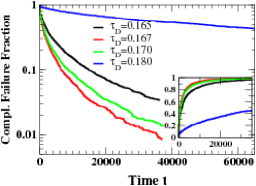
Figure 21: Complementary failure fraction $1-{\cal F}$ as a function of time for a range of delays $\tau_{D}$. The decay is non-exponential. Inset: Failure fraction ${\mathcal{F}}$ for the same data.

To obtain an approximate, analytic form for the failure fraction ${\cal F}(T^{*})$ we consider first - for a fixed value of $p$ - a single fixed configuration. The duration of the activity before failure will then depend on the specific initial condition chosen. In these simulations we choose 2,000 random initial conditions $V=V_{0}+\xi$ with $V_{0}=0.85$ and $-0.5<\xi<0.5$ picked from a uniform distribution. The resulting distribution for the failure times exhibits exponential behavior for large times. This allows the extraction of a characteristic failure time $T$ associated with this configuration. To reduce the computational effort these simulations are done in a smaller system with $N=200$. The exponential distribution suggests that the chaotic dynamics effectively lead to a fixed probability for the activity to die out after each population spike.

Across all configurations this leads then to a distribution $\rho(T)$ of characteristic failure times, in terms of which - averaged over many configurations - the fraction of failures up to a time $T^{*}$ is given by

$${\mathcal{F}}(T^{*})=\int_{0}^{\infty}dT\rho(T)(1-\beta e^{-\frac{T^{*}}{T}}).$$ (12)

Extracting the characteristic lifetimes $T$ of 50,000 configurations we find that the distribution $\rho(T)$ can also be well fit by an exponential function for long lifetimes,

$$\lim_{T\to\infty}\rho(T)\propto e^{-\alpha T}.$$ (13)

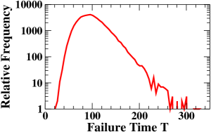
Figure 22: The distribution of characteristic failure times across 50,000 configurations. The distribution decays exponentially for long lifetimes. $N=200$, $p=1$, $\tau_{D}=0.16$

Fig.22 shows the result for $\tau_{D}=0.16$ and $p=1$ ($N=200$). Inserting the asymptotic behavior of Eq.(13) into Eq.(12) yields for large $t$

$${\cal F}(t)=1-2\beta\sqrt{\alpha t}K_{1}(2\sqrt{\alpha t})$$ (14)

where $K_{1}(x)$ is the modified Bessel function of the second kind of first order. For long times Eq.14 can be expressed as

$${\mathcal{F}}(t)\sim 1-\beta\sqrt{\pi}(\alpha t)^{1/4}e^{-2(\alpha t)^{1/2}}$$ (15)

displaying stretched exponential behavior. As Fig.23 shows, Eq.14 provides quite a good fit to the time dependence of the failure fraction. For $\tau_{D}=0.18$ the fit corresponding to $\alpha=0.67\cdot 10^{-5}$ and $\beta=0.91$ is good over essentially the whole range of times. For $\tau_{D}=0.165$ (inset) the fit is not quite as good; its curvature seems smaller than that of the data. Starting at $t=3,400$ one obtains $\alpha=0.12\cdot 10^{-3}$ and $\beta=0.64$. This fit overshoots the data for large times (blue dotted line in Fig.23). The fit with $\alpha=0.10\cdot 10^{-3}$ and $\beta=0.54$ (red dashed line) reduces the overshoot but is not as good for smaller times.

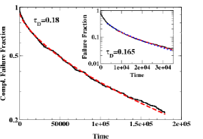
Figure 23: Complementary failure fraction $1-{\cal F}$ for $p=1$ and $\tau_{D}=0.18$ (inset for $\tau_{D}=0.165$). The dashed red and dotted blue lines show fits to Eq.(14).

V Conclusion

In this paper we have used a minimal model to study the influence of the network topology on the dynamics of excitable elements. The network consisted of local connections between neighboring elements on a ring that are supplemented by randomly chosen short-cuts connecting distant elements. Having neural systems in mind we have taken the short-cuts to provide uni-directional connections rather than the bi-directional ones that would arise in epidemic contexts Kuperman and Abramson (2001) or in regular diffusive processes.

Depending on the density of short-cuts and the speed of the waves propagating through this network we find three regimes. For low, but non-zero density of short-cuts the activity persists for essentially all network configurations when starting from an initial excitation of a single neuron. The activity is predominantly periodic and the mean firing rate of these states shows only little dependence on the wave speed or the density of short-cuts once $p\geq 0.05$ and it is reasonably close to the maximal firing rate allowed by the recovery period of the neurons. The recovery period is, however, not to be confused with an absolute refractory period; rather, it is the time after which synaptic input of the strength used in the computations is sufficient to trigger a new spike. This recovery period can be much longer than the usual absolute refractory period, for instance, if the neurons exhibit slow after-hyperpolarization as it underlies the slow oscillations ($<1$Hz) observed in vivo in cat Amzica and Steriade (1995) and in cortical slices of ferret Sanchez-Vives and McCormick (2000). There the relative refractory period induced by the after-hyperpolarization can last as long as a few seconds. The dependence of the propagation speed of such slow oscillations on the connectivity has been studied in cortical models Compte et al. (2003); Sanchez-Vives and Compte (2005). No true short-cuts were employed, instead the spatial width of the Gaussian giving the probability that two neurons are connected was varied Sanchez-Vives and Compte (2005) or a tri-modal probability distribution was used to capture a certain patchy connectivity in cortex Compte et al. (2003). As expected, the speed was found to increase with the width and it was conjectured that this connectivity dependence is the origin for the large difference observed for the slow waves in olfactory cortex and neocortex, respectively Sanchez-Vives and Compte (2005).

Even though for small numbers of short-cuts the long-time dynamics are periodic, the over-all behavior of the system can be quite complex due to the large number of stably coexisting solutions for a given network configuration. Whether the number of attractors grows as fast with the system size as in globally coupled oscillator networks, where the permutation symmetry essentially leads to a factorial growth of the number of attractors and to attractor crowding Wiesenfeld and Hadley (1989), is not known at this point. In fact, so far we have not been able to reach saturation of the number of attractors with increasing number of different initial conditions and the mechanism underlying this large number of attractors is not apparent yet. It is clear, however, that noise will induce a persistent switching between these different attractors Roxin (2003).

As the density is increased the number of network configurations that allow such a persistent activity decreases until essentially no persistent activity is possible anymore. For fast waves the transients after a localized excitation consist of a single population burst. For slower waves, however, for which the cross-over to complete failure occurs at yet larger short-cut densities, the transients can be exceedingly long comprising thousands of population bursts. The times at which the failures in activity averaged over different configurations occur are distributed according to a stretched exponential. It arises from the exponential distribution of the lifetimes characterizing each configuration. The mechanism responsible for these long transients presumably differs from that operating in diluted random networks of pulse-coupled oscillators Zumdieck et al. (2004).

While the fraction of failing configurations up to a given time follows a decreasing overall trend with decreasing wave speed, it exhibits intricate fine structure that includes even sharp, resonance-like increases of the failure fraction with decreasing wave speeds. This is surprising, since naively one might expect that a decrease in wave speed would allow additional, shorter loops to contribute to the activity and therefore enhance the chances for persistence. However, the result indicates that the activation of one loop can, in fact, make other, previously active loops impossible and thus induce failure. While it is clear that such a switching between loops can occur with increasing $\tau_{D}$, this mechanism is not yet understood in any detail.

The cross-over to failure, which can be understood analytically in detail based on a mean-field theory for the size of these idealized small-world networks, provides the basis for understanding a number of recent investigations employing more complex neural network models Netoff et al. (2004); Shao et al. (2006).

In Netoff et al. (2004) the connection between network connectivity and epilepsy in hippocampus was investigated by considering noisy and more elaborate versions of our model. It was found that for low numbers of short-cuts the noise drives only low-level activity, which was associated with normal behavior. With increasing short-cut density the activity strongly increased due to the recruitment of many more neurons by a noise-driven event. This activity was likened to seizing activity. This regime corresponds to the connectivities supporting persistent activity. Yet further increases in the short-cut density were found to induce bursting dynamics in which irregular bursts that involved a large fraction of all neurons are separated by periods of quiet. One would expect such a behavior for connectivities in the failing regime in which each noise-triggered event leads to a single population spike that brings essentially all neurons into the recovery period.

In Shao et al. (2006) the system was driven by a set of localized pace-maker neurons. It was found that the short-cuts can lead over a number of driving cycles to the build-up of bursts during which a large fraction of neurons fire within a small time window. The time to build up such bursts and the time between them was found to decrease with short-cut density. Again, the appearance of such bursts is related to the failing configurations in systems without driving. As expected from this observation the bursting behavior was supplanted by persistent activity when the wave speed was reduced (cf. Fig.12). The slow build-up towards the burst, however, is relatively specific to the Morris-Lecar model employed in that study for the individual neurons Shao et al. (2006).

We gratefully acknowledge support by NSF through grant DMS-0309657 and the IGERT program ”Dynamics of Complex Systems in Science and Engineering” (DGE-9987577) (HR,AR,SM) and by the EU under grant MRTN-CT-2004-005728 (SM).

References

- Albert and Barabasi (2002) R. Albert and A. L. Barabasi, Rev. Mod. Phys. 74, 47 (2002).
- Newman (2003) M. E. Newman, SIAM Rev. 45, 167 (2003).
- Barahona and Pecora (2002) M. Barahona and L. M. Pecora, Phys. Rev. Lett. 89, 054101 (2002).
- Nishikawa et al. (2003) T. Nishikawa, A. E. Motter, Y.-C. Lai, and F. C. Hoppensteadt, Phys. Rev. Lett. 91, 014101 (2003).
- Bressloff (2000) P. C. Bressloff, J. Math. Biol. 40, 169 (2000).
- Bressloff (2001) P. C. Bressloff, Physica D 155, 83 (2001).
- Golomb and Ermentrout (2001) D. Golomb and G. B. Ermentrout, Phys. Rev. Lett. 86, 4179 (2001).
- Traub et al. (1999) R. D. Traub, D. Schmitz, J. G. Jefferys, and A. Draguhn, Neuroscience 92, 407 (1999).
- Lewis and Rinzel (2000) T. J. Lewis and J. Rinzel, Network:Comput. Neural Syst. 11, 299 (2000).
- Lewis and Rinzel (2001) T. J. Lewis and J. Rinzel, Neurocomputing 38, 763 (2001).
- Perc (2005) M. Perc, New J. Phys. 7, 252 (2005).
- Lago-Fernández et al. (2000) L. F. Lago-Fernández, R. Huerta, F. Corbacho, and J. A. Sigüenza, Phys. Rev. Lett. 84, 2758 (2000).
- Lago-Fernández et al. (2001) L. F. Lago-Fernández, F. J. Corbacho, and R. Huerta, Neural Networks 14, 687 (2001).
- Carvunis et al. (2006) A. R. Carvunis, M. Latapy, A. Lesne, C. Magnien, and L. Pezard, Physica A 367, 595 (2006).
- Kuperman and Abramson (2001) M. Kuperman and G. Abramson, Phys. Rev. Lett. 86, 2909 (2001).
- Roxin et al. (2004) A. Roxin, H. Riecke, and S. A. Solla, Phys. Rev. Lett. 92, 198101 (2004).
- Watts and Strogatz (1998) D. J. Watts and S. H. Strogatz, Nature 393, 440 (1998).
- Netoff et al. (2004) T. I. Netoff, R. Clewley, S. Arno, T. Keck, and J. A. White, J. Neuroscience 24, 8075 (2004).
- Shao et al. (2006) J. Shao, T. Tsao, and R. Butera, Neural Comput 18, 2029 (2006).
- Tinsley et al. (2005) M. Tinsley, J. X. Cui, F. V. Chirila, A. Taylor, S. Zhong, and K. Showalter, Phys. Rev. Lett. 95, 038306 (2005).
- Steele et al. (2006) A. J. Steele, M. Tinsley, and K. Showalter, Chaos 16, 015110 (2006).
- Roxin (2003) A. Roxin, Ph.D. thesis, Northwestern University (2003).
- Wiesenfeld and Hadley (1989) K. Wiesenfeld and P. Hadley, Phys. Rev. Lett. 62, 1335 (1989).
- Newman et al. (2000) M. E. Newman, C. Moore, and D. J. Watts, Phys. Rev. Lett. 84, 3201 (2000).
- Newman and Watts (1999) M. E. Newman and D. J. Watts, Phys. Rev. E 60, 7332 (1999).
- Amzica and Steriade (1995) F. Amzica and M. Steriade, J. Neurophysiol. 73, 20 (1995).
- Sanchez-Vives and McCormick (2000) M. V. Sanchez-Vives and D. A. McCormick, Nature Neuroscience 3, 1027 (2000).
- Compte et al. (2003) A. Compte, M. V. Sanchez-Vives, D. A. Mccormick, and X. J. Wang, J. Neurophysiol. 89, 2707 (2003).
- Sanchez-Vives and Compte (2005) M. Sanchez-Vives and A. Compte, Lect. Notes Comp. Science 3561, 133 (2005).
- Zumdieck et al. (2004) A. Zumdieck, M. Timme, T. Geisel, and F. Wolf, Phys. Rev. Lett. 93, 244103 (2004).