Lotka-Volterra population model of genetic evolution

Abstract

A deterministic model of an age-structured population with genetics analogous to the discrete time Penna model [1, 2] of genetic evolution is constructed on the basis of the Lotka-Volterra scheme. It is shown that if, as in the Penna model, genetic information is represented by the fraction of defective genes in the population, the population numbers for each specific individual’s age are represented by exactly the same functions of age in both models. This gives us a new possibility to consider multi-species evolution without using detailed microscopic Penna model.

We discuss a particular case of the predator-prey system representing an ecosystem consisting of a limited amount of energy resources consumed by the age-structured species living in this ecosystem. Then, the increase in number of the individuals in the population under consideration depends on the available energy resources, the shape of the distribution function of defective genes in the population and the fertility age. We show that these parameters determine the trend toward equilibrium of the whole ecosystem.

PACS 87.23.-n, 87.53.Wz, 02.30.Hq

Keywords: Lotka-Volterra equations, Penna model, Evolution

1 Introduction

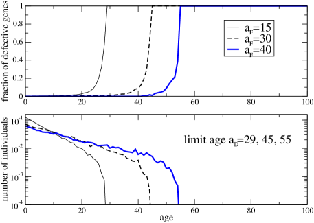
Figure 1: Monte Carlo simulation results of the Penna model of genetic evolution after $5\times 10^{7}$ MC steps. The upper panel shows the age-specific fraction of defective genes in three haploid populations with different values of the individual’s fertility age $a_{F}=15,30,40$. The remaining parameters of the Penna model are the same, $T=1$, $M=1$, bit-string length $n=100$. The resulting limit age of individuals in these populations $a_{D}=29,45,55$ is the age where the fraction of defective genes is equal to 1. The lower panel shows the age distribution in these populations.

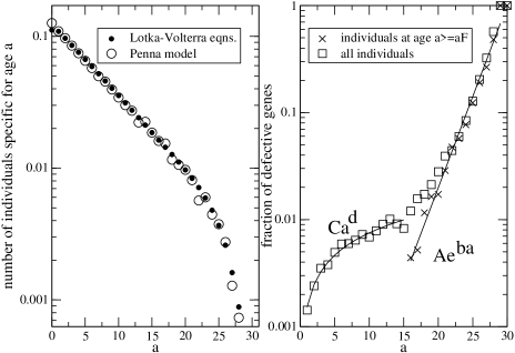
Figure 2: The dependence of the population number on the individual’s age in the case of the equilibrium Penna model of the bit-string evolution ($T=1$,$a_{F}=15$, $M=1$) and the age-structured Lotka-Volterra equations (the left panel of the figure). The right panel shows the distribution of defective genes in the equilibrium Penna model for the whole population and for individuals of age $\geq a_{F}$. The solid lines represent an approximation of the data $\varepsilon_{a}$ (fraction of defective genes in the population) which is power-like for the ages $a\leq a_{F}$ and exponential-like for $a>aF$.

Thousands of papers have been published on the Lotka-Volterra equations [3, 4] describing population growth, competition or speciation. In real populations the reproduction rate of individuals depends on their age and therefore it is necessary to include age structure into these equations. One example of how this can be achieved can be found in [5]. It is also possible to introduce a time delay between cause and effect (see, e.g. [6]). However, the majority of the Lotka-Volterra equations do not usually include genetic information and the question arises how to include it directly into the Lotka-Volterra equations.

The age-specific equations for population growth seem to be a good candidate to represent genetic information because the age structure introduces some analogy to the Penna model [1, 2] of genetic evolution. It is a model of genetic evolution although all details concerning the genes are skipped except of the state of their functionality - is the gene under consideration correct or it is mutated. This simple model has turned out to be very successful in interpreting the demographers data of real populations even as complex as human populations [2, 7, 8, 9].

In the original asexual version of the Penna model [1], the population under consideration consists of individuals represented by genomes defined as a string of $n$ bits. The bits represent states of genes where $0$ denotes its functional allele and $1$ its bad allele. It is assumed that if an individual possesses $T$ bad alleles switched on, it dies. In the model all genes are switched on chronologically - each bit corresponds to one ”year” - and maximum life span of an individual is $a_{D}$ ”years”. After reaching the fertility age $a_{F}$ an individual gives birth to $B$ offsprings whose genomes are mutated versions of the parental genome. The mutation rate $M$ is constant. After the mutation the affected gene is represented by a bit with a value opposite to the value before the mutation. The results of the Monte Carlo simulations of three different haploid populations for the Penna model in the case when back mutations from 1 to zero are not allowed have been shown in Fig. 1. In the figure, there have been plotted fraction of defective chronological genes in each population and age distribution of individuals.

In the diploid version of the Penna model the individual’s genome is represented by two bitstrings and then each locus possesses two alleles. The diploid individuals can reproduce sexually [2]. Both the haploid model of the equilibrium population and its diploid version are uniquely described by the fraction of defective genes in the population specific for each individual’s age. A short review of Monte Carlo simulation results for the Penna model with some additional details, like the presence of the housekeeping genes or the recombination frequency, can be found in [9].

Although the age distribution curves obtained in the Penna model coincide very well with demographers data for real populations, the model is not so “interdisciplinary” as the Lotka-Volterra population model. The reason could be that it is very difficult to obtain analytical results for the general Penna model and therefore one has to use the Monte Carlo method. However Monte Carlo simulations of the Penna model need large populations and the simulation time is very long. Hence, the typical multi-species problem exceeds the computing capability of a single PC-computer. Another problem is how to avoid the correlations arising from parallel computing if one tries to distribute the simulations to many processors. On the other side hand, it is relatively easy to solve numerically even a large set of the differential equations describing the Lotka-Volterra populations. Below we show how to include the fraction of defective genes into the equation for population growth so that the age distribution curves for these two models coincide.

In the following sections we discuss the behavior of the Lotka-Volterra ecosystem in which the age-specific species has been determined by the form of the fraction of defective genes.

2 Population growth of a single species

In this section we restrict ourselves to the haploid version of the Penna model but the results could be generalized to diploid populations. All we need from the Penna model is the distribution of defective genes in an equilibrium population and the corresponding age distribution. Such data could be taken from a real population as well. In the case of the Penna model we have performed a series of simulations of genetic evolution of the bitstring populations for different parameters like the fertility age $a_{F}$, genome length and the number of offsprings born each year. We considered the simplified case when the parameter $T=1$. The Verhulst factor was used to control the population size.

In the right panel of the Fig. 2 in the semi-log scale there have been plotted separately the fractions $\varepsilon_{a}$ of the age-specific defective genes in the whole equilibrium population and in the part of it which is consisting of the individuals with the age $a\geq a_{F}$. Fraction $\varepsilon_{a}$ of the age-specific defective genes in the whole equilibrium population and in the part consisting of individuals with $a\geq a_{F}$ are plotted in Fig. 2 on semilog axes. In the latter case all individuals should posses good genes specific for $a\leq a_{F}$ ($\varepsilon_{a}=0$) because $T=1$. Otherwise they should have died.

Our deterministic model for population growth is constructed in such a way that the values of the fractions $\varepsilon_{a}$ for each age $a=0,1,\ldots,a_{D}$ are inserted into the following set of the age-specific differential equations describing the change in number of individuals of age $a$:

$$\frac{dN_{a}(t)}{dt}=\alpha_{a-1}V(t)(1-\varepsilon_{a-1})N_{a-1}(t)-\gamma_{a}N_{a}(t),$$ (1)

where $N_{a}$ is the number of individuals specific for the age $a=1,\ldots,a_{D}$

$$N_{0}=\sum_{a\geq aF}N_{a}(t).$$ (2)

and $V$ represents the Verhulst saturation factor

$$V(t)=1-\frac{1}{\Omega}\sum_{a=1}^{a_{D}}N_{a}(t).$$ (3)

with $\Omega$ being the saturation level. The first term is the graduation term from the age $a-1$ to the age $a$ whereas the other part of the equation describes the graduation to the age $a+1$ and the individual’s mortality at age $a$. These terms are controlled by the age-specific rate coefficients $\alpha_{a}$ and $\gamma_{a}$, respectively. If we restrict the above to genetic evolution only, as in the case of the Penna model, we would have to choose the values $\gamma_{a}=1$ for all ages $a$, the reproduction rate $\alpha_{0}$ should be chosen as in the computer simulations of the Penna model (e.g. we set it to 1.1) but $\alpha_{a}=1$ for all ages $a>0$. The Verhulst factor (the same as in the Penna model) ensures that the solution of the equations Eq.(1) saturates at long times and then the age profile in the population coincides with the one from the equilibrium Penna population. An example of this can be observed in the left part of Fig. 2, where an analytical approximation of the simulation data $\{\varepsilon_{a}\}_{1}^{a_{D}}$ has been applied.

Equations Eq.(1) seem to possess many parameters. However, the simulations of the simple haploid version of the Penna model for different values of $a_{F}$ suggest that in the case of $T=1$ the fraction of the age-specific defective genes in the population which can be activated, i.e. after which the individuals die, consists of two parts (Fig. 2), one part relates to individuals of age $a\geq a_{F}$ and another one relates to individuals of age $a<a_{F}$. In this simple case we can approximate them as follows:

$$\varepsilon_{a}\sim Ca^{d}$$ (4)

for $a\leq a_{F}$ and

$$\varepsilon_{a}\sim Ae^{ba}$$ (5)

for $a>a_{F}$, with constants $A$, $b$, $C$, $d$. From the normalization condition, $\varepsilon_{a_{D}}=1$, we obtain

$$A=e^{-ba_{D}}.$$ (6)

Then, the number of parameters describing the fractions of defective genes drops down. It can be even smaller if we continue the left branch of the function $\varepsilon_{a}$ to $a=a_{F}+1$ and merge it with the right branch at $a=a_{F}+1$ in such a way that individuals of age $a\geq a_{F}$ did not contributed into the left branch also at $a=a_{F}+1$, i.e.

$$C(1+a_{F})^{d}-Ae^{1+aF}=Ae^{1+aF}.$$ (7)

Then we could estimate the value of the parameter $C$:

$$C=2Ae^{b(1+a_{F})}/(1+a_{F})^{d}.$$ (8)

In this way we have got an approximate distribution of defective genes controlled by four parameters, $b$, $d$, $a_{F}$ and $a_{D}$. In the equations Eq.(1) there is also the parameter $\alpha_{0}$, but it was kept constant and its value was the same as in the computer simulations of the Penna model.

The small number of parameters in the deterministic model makes it possible to consider multi-species evolution where the species differ in the values of $a_{F}$, $a_{D}$, $b$, $d$ and $\alpha_{0}$. In this case the numerical solutions do not require a high computational effort as in the Penna model. We should add that if the distribution function of the defective genes is an unknown function of $a$ and only the empirical values $\varepsilon_{a}$ are available, then these values could be used in the same way as in the discussed example, i.e., we do not need the analytical form of the distribution function for defective genes. We have considered only the case of the genetic evolution in equations Eq.(1) but there is a rich possibility to use other values of the coefficients $\alpha_{a}$ and $\gamma_{a}$ if one wants to describe real populations.

3 Predator-prey system

We consider an ecosystem in which a limited amount of the self-regenerating energy resources, $S(t)$, are consumed by the age-structured species living in this ecosystem. In this case, the increase in number of the individuals in the species depends on the available energy resources necessary for life processes. We will restrict ourselves to one species only. The species will carry genetic information represented by the fraction of defective genes in the population, the fertility age and the longevity $a_{D}$. We will show that the change of these genetic parameters can change the trend toward equilibrium of the whole ecosystem.

In the case of one species the ecosystem can be described by the following predator-prey set of equations

$$\frac{dS(t)}{dt}\,\,\, = \alpha_{S}S(t)\,(1-\frac{S(t)}{\Omega_{S}})-\gamma_{S}N(t)S(t)$$

$$\frac{dN_{a}(t)}{dt} = \alpha_{a-1}S(t)(1-\varepsilon_{a-1})N_{a-1}(t)-N_{a}(t),$$

where $a=1,\ldots,a_{D}$, $N_{0}$ is the same as in Eq.(2), $N(t)$ is the total number of individuals

$$N(t)=\sum_{a=1}^{a_{D}}N_{a}(t),$$ (10)

$S(t)$ represents energy units consumed by the species, $\Omega_{S}$ represents the saturation level for the energy resources, the coefficient $\alpha_{S}$ is the regeneration rate of the ecosystem resources, $\gamma_{S}$ is the damping coefficient due to the species using the energy resources. In order to follow the Penna model of genetic evolution the species evolves according to the equations Eq.(1) ($\gamma_{a}=1$ for all values of $a$) but the species’ growth is controlled by the amount $S(t)$ of the available energy resources instead of the Verhulst factor, $V(t)$. However, a Verhulst term is assumed for the self-regeneration of the ecosystem with respect to the energy resources. The energy resources represent prey and the species plays the role of predator. One could easily generalize the above set of equations to include many species.

We could expect that equations Eq.(LABEL:Ecosystem) have solutions which change in time in a similar way as the microscopic Penna model evolution in a limited ecosystem. We have recently studied an analogous predator - prey problem in [10], where a variable surrounding and its effect on the Penna model was considered. One of the findings of the computer simulations was that small changes in the inherited genetic information could lead to spontaneous bursts of evolutionary activity. The predator-prey dynamics with genetics could be as complex as discussed by Ray et al. [11] who showed that the system passes from the oscillatory solution of the Lotka-Volterra equations into a steady-state regime, which exhibits some features of self-organized criticality (SOC).

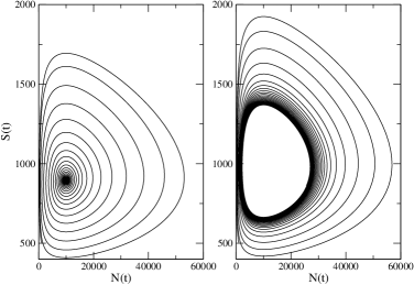
Figure 3: Both panels show the variation of the energy resources $S(t)$ and the total number of individuals $N(t)$ of the age structured species starting from the same initial conditions. The difference is that on the left $a_{F}=15$ and on the right $a_{F}=20$. The remaining parameters are the same, $a_{D}=29$ and $\alpha_{0}=1.1$.

In our model, we can always expect saturation of the energy resources if there is no species ($N(t)$=0) because the Verhulst term is present in Eq.(LABEL:Ecosystem). However, if $N(t)>0$ then depending on the shape of the distribution function of defective genes the solution of Eq.(LABEL:Ecosystem) saturates as in the example in the left part of Fig. 3 or it oscillates as in the right part of the figure. This means that an ecosystem with a few species can exhibit very complex evolution in which the solutions representing some species will spiral towards an equilibrium fixed point and some of them will try to converge to the limit cycle. The smaller the value of $a_{F}$ is, the larger the oscillations are, and the species may become extinct.

It is important that not only genetic parameters can change the type of the asymptotic solutions of Eq.(LABEL:Ecosystem). Consider a species similar to the one represented in the left hand part of, Fig. 3 for which the Lotka-Volterra solutions spiral to a fixed point. Let’s increase the value of the fertility age from $a_{F}$ to $a_{F}^{\prime}>a_{F}$ after some period of time but let the genetic information represented by the values $\{\varepsilon_{a}\}_{1}^{a_{D}}$ remain the same as before. For example, according to some social regulations since a specific time moment the individuals start to reproduce at older ages $a\geq a_{F}{\prime=20}$. The consequences of this shift in the reproduction age is that the solutions of Eq.(LABEL:Ecosystem) change qualitatively from the trend approaching the fixed point as in the left part of Fig. 3 to oscillations as in the case of the species from the right hand part of Fig. 3. It could happen that such a transition between these two types of solutions of the Lotka-Volterra equations could cause the species to become extinct.

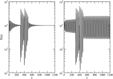
Figure 4: The effect of three catastrophes, where $30\%$ of the population under consideration has been eliminated at two time moments $t=300$ and $400$ and $10\%$ of the population at $t=500$. On the left there is a species with $a_{F}=15$ and $a_{D}=29$ and on the right the species has $a_{F}=20$ and $a_{D}=29$. In both cases the catastrophe at $t=500$ decreased the population number fluctuations.

In [12] it has been shown that the Lotka-Volterra systems have a self-regulatory character and there exist threshold values for the fraction of destroyed population above which the system returns to its previous state. We observe a similar behavior in our model. In particular, in Fig. 4 an effect of three such catastrophes on two different species represented by two different types of solutions of the Lotka-Volterra equations is shown. It is interesting that for some solutions the introduction of a perturbation decreases the amplitude of their oscillations. This could be observed in Fig. 4. The trace of this catastrophe in the $(S(t),N(t))$ representation has been shown in Fig. 5.

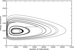
Figure 5: The effect of catastrophe from Fig. 4 on the variation of $S(t)$ and $N(t)$ in the population with $a_{F}=20$ and $a_{D}=29$.

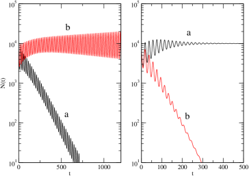
Figure 6: Dependence of population number $N(t)$ on time $t$ in the case of two species (a) and (b) competing for the same energy resources. In both figures, the species (a) has the same fertility age $a_{F}=15$ but $a_{D}=23$ on the left and $a_{D}=24$ on the right. The species (b) ($a_{F}=20$ and $a_{D}=29$) is the same in both cases. The same initial condition have been applied.

Thus, we could expect that in the ecosystem consisting of many species a rapid change like the extinction of a species or a sudden increase in their number can cause discontinuous changes of the fluctuations of the population numbers of the existing species, similarly as in Fig. 5 or Fig. 6 (discussed below). The age-specific structure of the competing populations seems to be an important factor in their survival.

It is easy to generalize the Lotka-Volterra equations Eq.(LABEL:Ecosystem) to the case of many species competing for the resources. If index $k$ runs through $M$ different species, the age-structured growth equations should be changed to the following:

$$\frac{dN_{a}^{k}(t)}{dt}=\alpha_{a-1}^{k}S(t)(1-\varepsilon_{a-1}^{k})N_{a-1}^{k}(t)-N_{a}^{k}(t),$$ (11)

where $k=1,2,\ldots,M$. Even in the case of two species $M=2$ the ecosystem under consideration can exhibit complex behaviour. For example, Fig. 6 shows the time dependence of the population number $N(t)$ for two competing species (a) and (b) in two cases which differ for species (a) by one parameter only, $a_{D}=23$ (left) and $a_{D}=24$ (right). The shift in the value of $a_{D}$ decides which species may become extinct.

4 Conclusions

It has been shown how to construct age-structured Lotka-Volterra equations in order to describe some features of genetic evolution. This could be helpful in modeling real populations where many parameters are typically used. In the considered model all species were competing for the same energy resources.

References

- [1] T.J.P. Penna, 1995. A Bit-String Model for Biological Aging. J. Stat. Phys. 78: 1629-1633
- [2] S. Moss de Oliveira, P.M.C. de Oliveira and D. Stauffer, 1999 Evolution, Money, War, and Computers, Teubner, Stuttgart-Leipzig
- [3] V. Volterra, Théorie mathématique de la lutte pour la vie, Gauthier-Villars, Paris, 1931
- [4] L.E. Reichl, A Modern Course in Statistical Physics, Edward Arnold (Publishers), 1980, pp. 641-644
- [5] D.C. Gazis, E.W. Montroll and J.E. Ryniker, 1973. Age-specific, Deterministic Model of Predator-Prey Populations: Application to Isle Royale. IBM J. Res. Develop., 47–53
- [6] P.J. Wangersky, 1978. Lotka-Volterra Population Models. Ann. Rev. Ecol. Syst., 9: 189–218
- [7] T.J.P. Penna, D. Stauffer, 1996. Bit-string ageing model and German population Zeitschrift für Physik B Condensed Matter 101: 469–470
- [8] K. Bońkowska, S. Szymczak and S. Cebrat, 2006. Microscopic modeling the demographic changes, Int. J. Mod. Phys. C 17 1477–1487
- [9] M. Kowalczuk, A. Łaszkiewicz, M. Dudkiewicz, P. Mackiewicz, D. Mackiewicz, N. Polak, K. Smolarczyk, J. Banaszak, M.R. Dudek and S. Cebrat, 2004. Using Monte Carlo simulations for the gene and genome evolution. Trends in Statistical Physics 4: 29–44
- [10] A. Nowicka, A. Duda, and M.R. Dudek, 2004. Effect of Variable Surrounding on Species Creation, C.R. Biologies 327:, 283–292
- [11] T.S. Ray, L. Moseley, N. Jan, 1998. A predator-prey model with genetics: transition to a self-organized critical state. Int. J. Mod. Phys. C 9: 701–710
- [12] A. Pekalski and D. Stauffer, 1998. Three Species Lotka-Volterra Model, Int. J. Mod. Phys. C 9: 777–784