Abstract

The apparent stability of population oscillations in ecological systems is a long-standing puzzle. A generic solution for this problem is suggested here. The stabilizing mechanism involves the combined effect of spatial migration, amplitude-dependent frequency, and noise: small differences between spatial patches, induced by the noise, are amplified by the frequency gradient. Migration among desynchronized regions then stabilizes the oscillations in the vicinity of the homogenous manifold. A simple model of diffusively coupled oscillators allows the derivation of quantitative results, like the dependence of the desynchronization upon diffusion strength and frequency differences. For an unstable system, a noise-induced transition is demonstrated, from extinction for small noise to stability if the noise exceeds some threshold. The coupled oscillator model is shown to reproduce all previously suggested stabilizing mechanisms. Accordingly, we suggest using this model as a standard tool for identification and classification of population oscillations on spatial domains.

I Introduction

The apparent stability of prey-predator systems is an age-old puzzle. While natural host-parasitoid and prey-predator systems persist for millions of years without extinction, simple considerations imply that this situation should be inherently unstable. Essentially, when a predator consumes a prey, it clearly increases its fitness and its chance to breed and produce more offspring. Thus, the predation rate should behave autocatalyticaly, leading to the extinction of the prey species and, consequently, the predator population. Even before the information and quantitative era, ancient day naturalists were able to recognize this puzzle. Among them, Herodotus and Cicero perceived the persistence of prey species in the face of adversity as a manifestation of divine power and the creator’s design (Cuddington, 2001). Herodotus’ explanation for the phenomenon was based on multiplication rates. In his words: ”… for timid animals which are a prey to others are all made to produce young abundantly, so that the species may not be entirely eaten up and lost; while savage and noxious creatures are made very unfruitful.” This explanation, clearly, can not stand on its own. Even if Herodotus’ statements about the reproduction habits of certain species were true (he claims that the hare is able to superfetete, i.e., to conceive while still pregnant; while the lioness may use her womb only once, since the cub ruptures it with his claws during pregnancy), balancing two exponentially divergent processes (multiplication and predation) is achievable only via fine-tuning of the parameters. Moreover, that fine-tuning must be robust against various kinds of noise. Indeed, as a rule, natural prey-predator systems are always subject to noise: either some sort of environmental stochasticity (e.g., years with more/less rain, weather fluctuations, heterogenous habitat) or, even under fixed conditions, some noise is introduced into the system due to demographic stochasticity, related to the discrete nature of the individual agents and the stochastic character of birth-death-predation processes (Lande, 2003; Foley 1997).

In modern times, the course of explanations has been changed, becoming more deterministic and quantitative. The basic idea relies on the fact that when the prey population decays there is not enough food for the predators and their population also diminishes, so both populations oscillate around their mean values. As pointed out by Nicholson (1933), these oscillations are an intrinsic property of interacting populations. If, for example, the density of a host is above its steady value, it will be reduced by the parasite. However, when the host reaches its steady density, the density of parasites is above its steady value. ”Consequently, there are more than sufficient parasites to destroy the surplus hosts, so the host density is still further reduced in the following generation … Clearly, then, the densities of the interacting animals should oscillate around their steady value.” This paradigm was formulated mathematically, using deterministic continuous-time partial differential equations (PDE’s), by Lotka and Volterra (LV model) (Lotka, 1920; Volterra 1931; Murray 1993). An analogous model with a discrete time step was introduced for a parasitoid-host system by Nicholson and Bailey (NB) (Nicholson and Bailey, 1935). Both models [and their variants (May, 1978; Hassell and Varley, 1969; Crowley, 1981; Rosenzweig and MacArthur, 1963)] allow for a coexistence fixed point, i.e., a steady state that admits finite population of the predator and the prey, and predict population oscillations around this coexistence steady state. The prediction of population oscillations is one of the major achievements of the deterministic models. Its most well known example is century-long documentation of oscillations in the Canadian lynx - Snowshoe Hare inhabitants of Northern America (Elton, 1924; Stenseth et al., 1998).

However, beyond this success, Lotka, Volterra and Nicholson recognized that their scheme fails to solve the basic stability problem, as it cannot account for the sustainability of these oscillations (Nicholson, 1933; Cuddington, 2001). If, under the influence of demographic or environmental stochasticity, oscillation amplitude increases, it should eventually reach an extinction point for one of the species. But this is exactly the situation for systems described by the Lotka-Volterra model: as oscillations of any amplitude are allowed, any type of noise will eventually increase their amplitude and the species will go extinct (see section 2 below). For the Nicholson-Bailey map, the situation is even worse: the coexistence fixed point is not only marginally stable but unstable. Thus, even without a continuous effect of noise, any small perturbation should increase exponentially and drive the system to extinction. Trying to maintain the coexistence state in a NB host-parasite model is like trying to balance a cone on its tip.

Facing the inability of the LV and NB models to admit oscillation sustainability, one may feel a temptation to abandon them altogether in favor of another formulation that supports an attractive fixed point or (if oscillations are required) a limit-cycle/strange-attractor. While it is reasonable to assume that some natural populations are described by such models, experimental and field studies show that, quite generically, this instability is a main characteristic of reality. In fact, for small systems and well-mixed populations, experiments show oscillation growth and extinction in a wide variety of interacting species (Gause , 1934; Pimentel et al., 1963; Huffaker, 1958). Spatially-extended systems, on the other hand, seem to support sustained oscillations, as emphasized by field studies, experiments, (Kerr et al., 2002; Kerr et al., 2006; Luckinbill, 1974; Holyoak and Lawler, 1996) and numerics (Wilson et al., 1993; Bettelheim et al., 2000; Washenberger et al., 2006; Kerr et al., 2002; Kerr et al., 2006).

These findings give an appeal to Nicholson’s (1933) old proposal about migration induced stabilization, i.e., that desynchronization between weakly coupled spatial patches, together with the effect of migration, stabilize the global populations. To get the flavor of the mechanism, let us imagine a metapopulation on two patches, where within each patch the population oscillations are governed by, say, Lotka-Volterra dynamics with constant diffusion (i.e., constant per capita migration rate) between these two patches. Clearly, as emphasized in Figure 1, if the oscillations on these two patches desynchronized, e.g., if one of the patches is in a state of large populations while the other is, at the same time, in a diluted state, migration between patches pushes the whole system inward toward the coexistence fixed point yielding sustained oscillations. However, one should bear in mind that migration is a double edged sword, as it tends to avoid population gradients and leads to synchronization. The acid test for Nicholson’s proposal is thus as follows: is the diffusion among patches weak enough to allow noise-induced desynchronization, but at the same time strong enough to stabilize desynchronized patches? If this is to be the case, the desynchronization-diffusion stabilization may work.

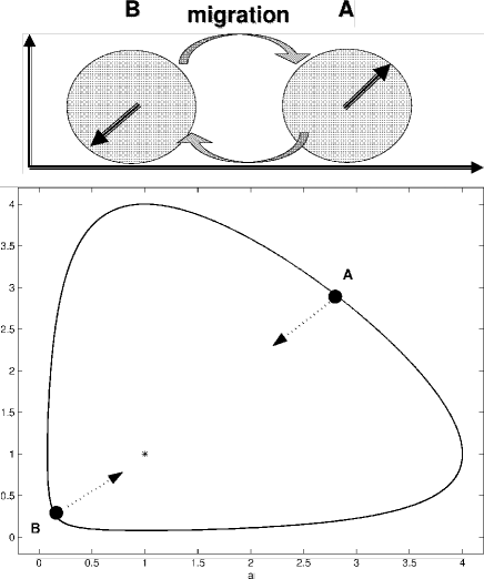
Figure 1: Population oscillation on two spatial patches coupled by migration. If both patches desynchronize, one may find one of them (A) in the dense population state and the other one (B) in the dilute phase. Diffusion tends to decrease population gradients, hence the whole system flows towards the coexistence fixed point, represented in the lower panel by an asterisk.

Unfortunately, examination of this idea in many studies, summarized in a recent review article (Briggs and Hoopes, 2004), yields negative results. Generically, diffusion stabilizes the homogenous manifold and different spatial patches get synchronized, leading back to the well-mixed unstable dynamics (Crowley, 1981; Allen, 1975; Reeve, 1990). At the end of the day, thus, we are back where Herodotus left us more than 2500 years ago: we cannot explain the sustainability of prey-predator systems, despite their presence since the beginning of life on earth. The understanding of oscillation persistence is not only an intellectual challenge; stabilization of such oscillations is considered to be a major factor affecting species conservation and ecological balance (Earn et al., 2000; Blasius et al., 1999).

The goal of this paper is to provide a generic solution to this puzzle, a solution that is independent of external assumptions, such as space-time fluctuations or heterogenous migration patterns. We will show that the basic ingredient that leads to desynchronization is the dependence of oscillation frequency on their amplitude (Amplitude Dependent Frequency, ADF), and will survey the consequences and the implementation of this idea for different systems and types of noise. The basic quantitative and qualitative tool presented here is a simple toy model for coupled oscillators. Apart from its usefulness in the analysis of the ADF mechanism, this toy model works for all types of stabilizing mechanisms presented so far, and serves as a prediction and classification tool. As such, we suggest our coupled oscillators system to be used as the standard -modeling technique for metapopulation oscillations.

The present work is organized as follows: in the next section, the stability problem will be introduced for a single patch system, together with a short review of the experimental and numerical results that support the instability for well-mixed populations. In the following section, Nicholson’s proposal - desynchronization induced stability on spatial domains - is endorsed, based again on numerics and experimental results. The fourth section is the main part of the paper, where a toy model is presented and analyzed and the role of amplitude-dependent oscillations is clarified. Next we give a short critical review of previous solutions to the stability problem, and show how to incorporate them all within the framework of diffusively-coupled oscillators. We end up with some concluding remarks, trying to sketch a classification scheme for observed population dynamics in experimental and numerical situations.

II Instability and extinction of well mixed populations

We begin the demonstration of the instability problem looking at the Lotka-Volterra predator-prey system, the paradigmatic model for oscillations in population dynamics (Lotka, 1920; Volterra, 1926; Murray, 1993). The model describes the temporal evolution of two interacting populations: a prey ($b$) population that grows with a constant birth rate $\sigma$ in the absence of a predator (the energy resources consumed by the prey are assumed to be inexhaustible), while the predator population ($a$) decays (with death rate $\mu$) in the absence of a prey. Upon encounter, the predator may consume the prey with a certain probability. Following a consumption event, the predator population grows and the prey population decreases. For a well-mixed population, the corresponding partial differential equations are:

$$\frac{\partial a}{\partial t} = -\mu a+\lambda_{1}ab$$ (1)

$$\frac{\partial b}{\partial t} = \sigma b-\lambda_{2}ab$$

where $\lambda_{1}$ and $\lambda_{2}$ are the relative increase (decrease) of the predator (prey) populations due to the interaction between species, correspondingly.

The system admits two unstable fixed points: an absorbing state $a=b=0$ and the state $a=0,\ \ b=\infty$. There is one coexistence, marginally stable fixed point at $\bar{a}=\sigma/\lambda_{2},\ \ \bar{b}=\mu/\lambda_{1}$. Local stability analysis yields the eigenvalues $\pm i\sqrt{\mu\sigma}$ for the stability matrix. Moreover, even beyond the linear regime there is neither convergence nor repulsion. Using logarithmic variables $z=ln(a),\ q=ln(b)$ eqs. (1) take the canonical form $\dot{z}=\partial H/\partial q,\ \ \dot{q}=-\partial H/\partial z$, where the conserved quantity $H$ (in the $ab$ representation) is:

$$H=\lambda_{1}b+\lambda_{2}a-\mu\ ln(a)-\sigma\ ln(b).$$ (2)

The phase space is thus segregated into a collection of nested one-dimensional trajectories, where each one is characterized by a different value of $H$, as illustrated in Figure 2. Given a line connecting the fixed point to one of the ”walls” (e.g., the dashed line in the phase space portrait, Figure 2), $H$ is a monotonic function on that line, taking its minimum $H_{min}$ at the marginally stable fixed point (center) and diverges on the wall. It turns out that all the important features related to the instability and the synchronization depend only on the topology of the phase space, and the actual values of the growth, death and predation parameters are not important. Thus, without loss of generality, we employ hereon (unless otherwise stated) the symmetric parameters $\mu=\sigma=\lambda_{1}=\lambda_{2}=1$. The corresponding phase space, along with the dependence of $H$ on the distance from the center and a plot of the oscillation period vs. $H$, are represented in Figure 2.

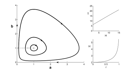
Figure 2: The Lotka-Volterra phase space (left panel) admits a marginally stable fixed point surrounded by close trajectories (three of these are plotted). Each trajectory corresponds to a single $H$ defined in Eq. (2), where $H$ increases monotonically along the (dashed) line connecting the center with the $a=0$ wall, as shown in the lower right panel. In the upper right panel, the period of a cycle $T$ is plotted against $H$, and is shown to increase almost linearly from its initial value $T=2\pi/\sqrt{\mu\sigma}$ close to the center.

Given the integrability of that system, the effect of noise is quite trivial: if $a$ and $b$ randomly fluctuate in time, the system wanders between trajectories, thus performing some sort of random walk in $H$ with ”repelling boundary conditions” at $H_{min}$ and ”absorbing boundary conditions” on the walls (as negative densities are meaningless, the ”death” of the system is declared when the trajectory hits the zero population state for one of the species, i.e., when at least one of the species becomes extinct). Thus, under the influence of noise, thus, the problem is reduced to that of a random walk with an absorbing trap [a first passage problem (Redner, 2001)]. While the first passage problem is characterized by power law decay, here the topology of the orbits forces the trajectory back to the vicinity of the absorbing walls, and hence the decay is exponential. An example of a phase space trajectory for a single patch noisy LV system is shown in the inset of figure 3, and the average growth of the oscillation amplitude is clearly seen. The survival probability $Q(t)$ (the probability that a trajectory does not hit the absorbing walls within time $t$) is shown for different noise amplitudes in figure 3.

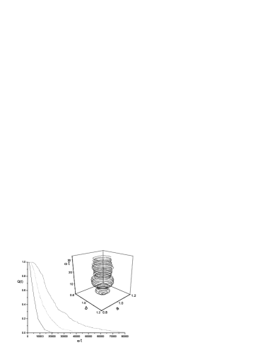
Figure 3: The survival probability $Q(t)$ is plotted versus time for a single patch noisy LV system. Eqs. (1) (with the symmetric parameters) were integrated numerically (Euler integration with time step $0.001$), where the initial conditions are at the fixed point $a=b=1$. At each time step, a small random number $\eta(t)\Delta t$ was added to each population density, where $\eta(t)\in[-\Delta,\Delta]$. A typical phase space trajectory, for $\Delta=0.5$, is shown in the inset. The system ”dies” when the trajectory hits the walls $a=0$ or $b=0$. Using 300 different noise histories, the survival probability is shown here for $\Delta=0.5$ (full line), $\Delta=0.3$ (dotted line) and $\Delta=0.25$ (dashed line). Clearly, the survival probability decays exponentially at long times, $Q(t)\sim exp(-t/\tau)$, as expected for a random walk with absorbing boundary conditions, $1/\tau$ scales with $\Delta^{2}$.

At this point it is instructive to clarify the types of noise to be used throughout this paper. The first and the most simple is the additive noise, i.e., random addition or subtraction of population density at certain time steps. In the real world, this corresponds to migration of small parts of the population in and out of the considered system. As the implementation of an additive noise in Langevin type equations is relatively simple, we use it as the ”noise of choice” for the present work.

Indeed, there are two common sources for time-dependent randomness in ecological systems. One source is the environmental stochasticity, i.e., fluctuations in the environmental conditions that may change the reaction and interaction parameters. The growth rate of the prey, for example, should be taken not as a constant $\sigma$ but as a fluctuating quantity around some average, $\langle\sigma\rangle+\delta\sigma(t)$, where $\langle\cdots\rangle$ stands for average over time. Another source of noise is the intrinsic demographic stochasticity. While Eqs. (1), for example, describe continuous populations sizes $a(t)$ and $b(t)$ that may take any value, the actual number of individuals in a community should be an integer (Lande et al., 2003). Indeed, Partial differential equations like (1) only describe the dynamic of the average population and are derived from the exact master equation as a ”mean field” approximation, neglecting higher correlations and approximating, e.g., $\langle a(t)b(t)\rangle\sim\langle a(t)\rangle\langle b(t)\rangle$. The actual dynamics of the system, described by the master equation, is not deterministic but stochastic, and this implies that noise of order $\sqrt{N}$ is applied to any population of $N$ individuals. While the relative amplitude of that noise decays like $1/\sqrt{N}$ for large populations, it is still of importance if there is no attractive manifold for the deterministic dynamics (Kessler and Shnerb 2006), such as in the LV or NB models. The effect of demographic stochasticity on a single path LV system is very similar to that of additive noise, as indicated by the simulation results obtained using Gillespie’s event driven algorithm (Gillespie, 1977).

In the current work, additive noise is used in order to model multiplicative noise such as demographic stochasticity. This procedure may be justified using a self-consistency argument: we want to present a mechanism that stabilizes the population oscillations, such that the number of individuals in, say, the predator population, does not deviate strongly from its average value. If this is the case, the ${\cal O}(\sqrt{N})$ noise amplitude does not change so much along the orbit and the system ”feels” constant (additive) noise. The noise amplitude of environmental stochasticity is proportional to the population size [the term $\delta\sigma(t)$ presented above multiplied by the prey population in (1)], thus it is also approximated by an additive noise with a constant amplitude if the oscillations are not too large.

While the LV system is marginally stable and is driven to extinction by the noise, the situation for the host-parasitoid model of Nicholson and Bailey is even worse. In their model, the host population $H$ and the parasite population $P$ satisfy the map (Nicholson and Bailey, 1935):

$$H_{t+1}=\sigma H_{t}e^{-\lambda P_{t}},$$

$$P_{t+1}=cH_{t}(1-e^{-\lambda P_{t}})$$ (3)

where $\sigma>1$ is the growth factor of the host in the absence of a parasite. The system admits a coexistence fixed point at:

$$H=\frac{ln\ \sigma}{\lambda},$$

$$P=\frac{\sigma ln\ \sigma}{c\lambda(\sigma-1)}.$$ (4)

and small deviations from that fixed point grow exponentially with time, yielding a prompt extinction of one of the interacting species (see Figure 4). Here the effect of noise is negligible: any infinitesimal deviation from the fixed point renders the system extinction-prone.

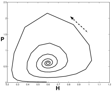
Figure 4: Nicholson-Bailey dynamics. The map (II) is iterated 90 times where the initial deviation from the fixed point is 0.001. The parameters are $\sigma=1.2$, $\lambda=0.3$, $c=6.1$.

III Spatial structure and sustained oscillations

As concluded in the last section, a well-mixed population that obeys Lotka-Volterra or Nicholson-Bailey dynamics is extinction prone: oscillation amplitude grows in time until one of the species goes extinct. The only difference between the two models is the way this extinction is approached: while an NB system is unstable and oscillations grow in time exponentially even without noise, the LV model admits neutral oscillations and approaches extinction only due to the effect of stochasticity.

One may thus suggest that something is wrong in the modeling of interspecific interaction. While LV and NB are clearly the simplest descriptions of the corresponding systems, maybe in nature some more complicated processes take place, and more accurate mathematical models should use equations that support an attractive manifold, i.e., a phase space region that ”attracts” the trajectories. In particular, one may write a model that supports a stable fixed point, limit cycle (Kolmogorov, 1936; May, 1972) or strange attractor. In the first case, after a short period of oscillations the system settles into a stable state of constant populations; in the second, it will converge to fixed amplitude oscillations; and in the third scenario (strange attractor), it will wander chaotically between a set of points confined to some phase space region. Any of these solutions is robust against small noise, as the dynamic is dissipative, small fluctuations flow back into the attractive manifold.

However, a series of experimental results shows that, indeed, for small sample sizes, prey-predator or host-parasitoid systems actually flow to extinction. From the seminal work of Gause on the Didinium - Paramecium system (Gause, 1934), through Huffaker’s orange experiment (six spotted mite - Typhlodromus ) (Huffaker, 1958), and Pimintel’s wasp-fly setup (Pimentel et al., 1963); all of these experiments demonstrated that population dynamics result in extinction of one of the species.

Of particular interest is a new series of experiments dealing with the cyclic, rock-paper-scissors dynamic (Kerr et al., 2002; Kirkup and Riley, 2004; Kerr et al., 2006) . In the first set of experiments, colicin-producing strains (C) of E. Coli were interacting with colicin-sensitive (S) and colicin-resistent strains (R); while C kills S, S outcompetes R and R wins against C. It turns out that for well-mixed systems, both in vitro (Kerr et al., 2002) and in vivo (Kirkup and Riley, 2004), fluctuations drive two of the three species to extinction via the same mechanism of ”random walk” among naturally stable orbits (Reichenbach et al., 2006). In the second experiment (Kerr et. al., 2006) E. Coli and its parasitoid (phage) were subjected to controlled migration. Again, in the ”well-mixed” regime, when all the biological materials were mixed each 12 hours, extinction took place after a very short time.

On the other hand, the spatial structure and, in particular, spatial migration have been shown to be of crucial importance in the sustainability of interacting populations. The famous field studies about natural prey-predator systems [like the Canadian Lynx - Snowshoe Hare (Elton, 1924; Stenseth et. al., 1998) data from Hudson Bay company, the Moose-Wolf coexistence in Isle Royal (Wilmers, et al., 2006), and the biological control of the Prickly pear cactus by the moth cactoblastis cactorum in eastern Australia (Freeman, 1992)] indicate that, in spatially-extended systems, the population oscillations are either negligible or finite, ensuring persistence. Luckinbill’s (Luckinbill, 1974) experiment, using again the Didinium - Paramecium system, shows that the system’s lifetime (time until extinction of one of the species) grows almost exponentially with its linear size. Similar observations were made by Holyoak and Lawler (1996), and, as already mentioned, by the series of experiments dealing with rock-paper-scissors dynamics (Kerr et. al., 2002; 2006) , where slow mixing yields finite fluctuations and promotes survival. There are also many numerical experiments on stochastic models (like the individual-based models, subject to demographic stochasticity) that show stable oscillations for large samples(Wilson, et al., 1993; Bettelheim et al., 2000; Washenberger et al., 2006 ;Kerr et. al., 2002; 2006).

All in all, much evidence supports the idea that interacting species dynamics are inherently unstable on a single patch, and that the stability observed in nature is related to the fact that natural systems are spatially-extended. This idea may be implemented in an extinction-recolonization scenario (Taylor, 1990), but in general this mechanism works for any system that supports desynchronization. As pointed out by Nicholson (1933), if the system desynchronizes, the migration between patches will induce an inward flow toward the coexistence fixed point and stabilize the amplitude of oscillations. The main puzzle, thus, is reduced to the identification of the conditions under which desynchronization takes place. It turns out, however, that generically the diffusion tends to lock the system to its synchronized state, stabilizing the homogenous manifold such that the whole system acts like a single patch, rendering unbounded oscillations (Briggs and Hoopes , 2004).

The condition for desynchronization in diffusively coupled patches have been examined in many studies and the main results, summarized in a recent review article (Briggs and Hoopes , 2004), are as follows:

• For any network of $N$ patches, if the migration between patches is symmetric or almost symmetric (i.e., the diffusion of the prey and the predator are, more or less, the same), there is no diffusion-induced instability, and the homogenous manifold is stable (Crowley, 1981; Allen, 1975; Reeve, 1990). Thus, the effect of migration alone does not cure the instability problem.

• The system may become desynchronized when in the presence of spatial heterogeneity, e.g., where the reaction parameters vary on different spatial patches (Murdoch and Oaten, 1975; Murdoch et al., 1992; Hassell and May, 1988). In that case, the intrinsic dynamic at any localized patch takes place on different time scales for the same concentrations, so diffusion fails to synchronize different patches. This mechanism may be generalized to include not only ”quenched” heterogeneity but also environmental stochasticity, i.e.,where the reaction parameters are subject to spatio-temporal fluctuations (Crowley, 1981 ; Reeve, 1990; Taylor, 1998) .

• Spatial heterogeneity may be introduced into the model in a more sophisticated way: one may define a homogenous dynamics in all patches with an underlying nonlinear process that supports spontaneous symmetry breaking and pattern-formation. These patterns, in turn, will control the reaction parameters to yield desynchronization.

• Diffusion-induced instability may occur if the migration rate of the predator is much smaller than that of the prey, particulary if the prey migration rate is zero [Jansen, 1995; Abta et al. (2006 b)].

While spatial heterogeneity, environmental stochasticity, and different migration rates for different species are indeed characteristics of many natural systems, these mechanisms are not generic and it seems that they cannot explain the experimental results that show persistence in ”clean” extended systems, like (Luckinbill, 1974) and (Kerr et al.; 2002; 2006). Accordingly, it seems that the combined effect of noise and diffusion is a necessary precondition for population stabilization. However, up until now, the qualitative nature of the ”missing” underlying mechanism has remained obscure, and no theoretical framework that allows for quantitative prediction has been presented.

This theoretical gap has been addressed recently (Abta et al., 2006 a) using a toy model for coupled oscillators presented in the next section. The main new ingredient emphasized by the proposed model is the dependence of frequency on the oscillation amplitude, reflected by the gradient of the angular velocity along the radius $\omega^{\prime}(r)$. The instability induces desynchronization iff the small, noise-induced differences between patches are amplified by the frequency gradient such that the ”desynchronization parameter” $\langle\phi^{2}\rangle$ acquires a finite value, leading to ”restoring force” toward the origin of the homogenous manifold.

Moreover, it turns out that our toy model may also reproduce the other mechanisms suggested in the past, and yield simple analytical results together with qualitative and quantitative predictions. In the fifth section, these generalizations are presented. Thus, our toy model allows for a comprehensive typification of different mechanisms for sustained oscillation on diffusively coupled patches, and yields simple criteria for classification of experimental results and identification of the stabilizing mechanism.

IV Two patch system

To consider the effect of spatial structure, let us begin with the simplest case, i.e., two patch system connected diffusively as in Figure 1. One should bear in mind, though, that any finite system that admits an absorbing state and is subject to additive noise must eventually reach extinction. Under the influence of noise, any stable state becomes only metastable, as some rare configuration of the noise will push one of the species to extinction. The appearance of sustained oscillations, i.e., of an attractive manifold, manifests itself in finite system only in its lifetime before it hits the absorbing state. This lifetime, $\tau$, is known in the literature as the ”intrinsic mean time to extinction” (Grimm and Wissel, 2004), and if a metastable state appears, it increases exponentially with the ”strength” of attraction (the Lyapunov exponent) of that manifold. If the stability of a system increases with the number of patches, one may expect the lifetime of the system to diverge with the number of patches, yielding real stability for an infinite system. The best example of this phenomenon - a metastable state in a small system becoming stable as its size grows - is the logistic growth with demographic stochasticity, where the transition from extinction to proliferation belongs to the directed percolation equivalence class (Grassberger, 1982; Janssen, 1981). A similar transition, belonging to the same universality class, was observed recently for coupled limit cycles with demographic stochasticity (Mobilia, et al, 2006). Thus we are not trying to show that the two patch system is really stable; exponential growth in the lifetime of the system is a clear indication of the appearance of an attractive manifold that yields real stability in the infinite size limit.

The simplest example is the LV system on two patches:

$$\frac{\partial a_{1}}{\partial t} = -\mu a_{1}+\lambda_{1}a_{1}b_{1}+D_{a}(a_{2}-a_{1})$$

$$\frac{\partial a_{2}}{\partial t} = -\mu a_{2}+\lambda_{1}a_{2}b_{2}+D_{a}(a_{1}-a_{2})$$ (5)

$$\frac{\partial b_{1}}{\partial t} = \sigma b_{1}-\lambda_{2}a_{1}b_{1}+D_{b}(b_{2}-b_{1})$$

$$\frac{\partial b_{2}}{\partial t} = \sigma b_{2}-\lambda_{2}a_{2}b_{2}+D_{b}(b_{1}-b_{2}).$$

The time evolution of that system, with additive noise, equal diffusivities, $D_{a}=D_{b}\equiv D$, and symmetric reaction rates is obtained through Euler integration. In the limit $D=0$ the patches are unconnected; thus, starting from the homogenous fixed point $a_{1}=a_{2}=b_{1}=b_{2}=1$, the single patch situation still holds and the system hits the absorbing walls after a characteristic, noise-dependent, time. In the opposite limit, $D=\infty$, the system sticks to the invariant manifold and acts like a single patch (with modified noise and interaction parameters), again performing a random walk in the invariant manifold. However, between these two extremes, there is a region where the combined effect of diffusion and noise stabilizes a finite region within the invariant manifold. For any noisy two-patch system $Q(t)$, histograms (like those shown for a single patch in Figure 3) were used to extract the typical decay time [”intrinsic mean time to extinction” (Grimm and Wissel, 2004)] $\tau(D,\Delta)$ by fitting its tail to exponential decay $exp(-t/\tau)$. In Figure 5, $\tau(D,\Delta)$ is plotted against $D$ for different noise amplitudes, and is shown to increase (faster than exponentially) with $D$ ($1/D$) as $D$ approaches zero (infinity). Evidently, for intermediate diffusivities, an attractive manifold appears in phase space, with a Lyapunov exponent that grows (faster than linearly) with the diffusion constant.

Figure 5: The typical persistence time as a function of the diffusion rate for different levels of noise. The values of $\tau$ were gathered from survival probability plots (like those in Figure 3) and are displayed here for the two-patch system. One sees that the value of $\tau$ grows very rapidly (even faster than exponentially) with the migration rate for small diffusion values, and decays with $D$ for large diffusivities. Data is shown for different noise intensities $\Delta=0.3$ (triangles), $0.5$ (squares) and $1.0$ (circles).

IV.1 The Coupled oscillator model and LV system

Although both the Lotka-Volterra and Nicholson-Bailey models are oversimplified with respect to the complexity of interspecies interactions in the natural world, they are still too complicated to allow for an understanding of the stabilization mechanism when migration and noise interfere. The main obstacle (as will become clear later) is that the radial velocity along a trajectory depends not only on the amplitude of oscillations (related to the conserved quantity $H$), but also on the location along a trajectory, i.e., on the azimuthal angle between the point along the trajectory and the fixed point $\theta$ (see Figure 6). In order to clarify the origin of the stable cycles, let us introduce a toy model that imitates the main features of the real systems. Although that model does not allow for an absorbing state, it captures the basic mechanism for stabilization of spatially-extended systems in the presence of noise.

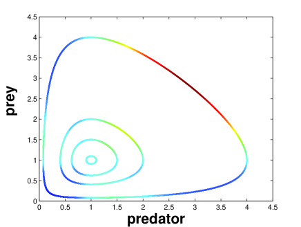
Figure 6: The angular velocity along some orbits of the Lotka-Volterra dynamic. Fast regions are marked in red, slow regions in blue. Clearly, the dynamic is slowest when the populations of both species are diluted, and fastest along the dense region in the upper-right ”shoulder.” Note that the velocity gradient along an orbit increases with $H$.

The toy model deals with the phase space behavior of diffusively-coupled oscillators, where the angular frequency depends on the radius of oscillations. With additive noise, the Langevin equations take the form,

$$\frac{\partial x_{1}}{\partial t} = \omega(x_{1},y_{1})y_{1}+D_{1}(x_{2}-x_{1})+\eta_{1}(t)$$

$$\frac{\partial x_{2}}{\partial t} = \omega(x_{2},y_{2})y_{2}+D_{1}(x_{1}-x_{2})+\eta_{2}(t)$$

$$\frac{\partial y_{1}}{\partial t} = -\omega(x_{1},y_{1})x_{1}+D_{2}(y_{2}-y_{1})+\eta_{3}(t)$$ (6)

$$\frac{\partial y_{2}}{\partial t} = -\omega(x_{2},y_{2})x_{2}+D_{2}(y_{1}-y_{2})+\eta_{4}(t),$$

where all the $\eta$-s are taken from the same distribution. If the angular frequency is location independent, $\omega(x,y)=\omega_{0}$, the problem is reduced to coupled harmonic oscillators, a diagonalizable linear problem that admits two purely imaginary eigenvalues in the invariant, homogenous manifold. With noise, the random walk on that manifold is independent of the motion in the fast manifold and the radius of oscillation diverges with the square root of time.

Now let us define the oscillation radius for each patch, $r_{i}=\sqrt{x_{i}^{2}+y_{i}^{2}}$ for $i=1,2$, and assume that the angular frequency depends only on that radius and is $\theta$-independent [$\theta_{i}\equiv arctg(y_{i}/x_{i})$]. With that, the total phase $\Phi=\theta_{1}+\theta_{2}$ decouples and the 3-dimensional phase space motion is dictated by the equations (we take $D_{1}=D_{2}=D$ and define $\phi=\theta_{1}-\theta_{2}$, $R\equiv r_{1}+r_{2}$, $r\equiv r_{1}-r_{2}$):

$$\dot{R} = -2Dsin^{2}(\phi/2)R+\tilde{\eta}_{R}$$ (7)

$$\dot{r} = -2Dcos^{2}(\phi/2)r+\tilde{\eta}_{r}$$ (8)

$$\dot{\phi}=-2 D \left(\frac{R^{2}+r^{2}}{R^{2}-r^{2}}\right)sin\phi+\omega(r_{2})-\omega(r_{1})+\left(\frac{\tilde{\eta}_{1}}{r_{1}}-\frac{\tilde{\eta}_{2}}{r_{2}}\right).$$ (9)

As before, all the $\tilde{\eta}$-s are taken from the same distribution. Note that $\phi$ represents the phase desynchronization between patches while $r$ is the amplitude desynchronization.

Eqs. (7) clarify the role of phase desynchronization as the stabilizing mechanism. The dynamics in the homogenous ($R$) manifold look very much like that of an overdamped harmonic oscillator in noisy environment,

$$\dot{z}=-kz+\eta(t),$$ (10)

a well-known system [Ornstein-Uhlenbeck process, (Gardiner, 2004)] that admits the steady state Boltzman distribution $P(z)\sim exp(-kz^{2}/\Delta^{2})$. However, if the phases of these two patches synchronize and the expectation value of $\phi^{2}$ vanishes, so does the ”spring constant” of the oscillator. Without that restoring force, the motion on the $R$ manifold is a simple random walk, so the oscillation amplitude grows indefinitely. Phase ($\phi$) desynchronization, thus, is the crucial condition for stabilization. This feature is stressed in the inset of Figure 7, where the flow lines of the deterministic dynamics in the $R-\phi$ plane are sketched: the line $\phi=0$ is marginally stable, but any deviation leads to inward flow.

Close to the invariant manifold, when $\phi$ and $r/R$ are much smaller than one, the amplitude desynchronization $r$ is solvable. Neglecting corrections of order $\phi^{2}$,

$$\dot{r}=-2Dr+\eta,$$ (11)

which is again an equation for an overdamped harmonic oscillator, so

$$P(r)\sim exp(-Dr^{2}/\Delta^{2})$$ (12)

and the $r^{2}$ typical fluctuation around zero is of order $\Delta^{2}/D$. However, the amplitude desynchronization factor $r$ does not appear in (7), and the stabilization is determined only by the phase. Accordingly, the system supports an attractive manifold iff the amplitude desynchronization yields phase desynchronization.

Another piece of information may be gathered from the harmonic limit, $\omega(r)=\omega_{0}$. Here there should be no phase synchronization, as we already diagonalized the linear equation and find no restoring term in the homogenous plane. Looking at Eq. (9) with $\omega(r_{1})-\omega(r_{2})=0$ one concludes, thus, that the rightmost (noise) term in (9) is irrelevant. The dependence of the frequency on the amplitude (i.e., the dependence of $\omega$ on $r$) should be the factor that allows the translation of amplitude desynchronization into a phase desynchronization. Intuitively, when two patches with different oscillation amplitudes move with different angular velocities, this immediately yields phase differences.

Figure 7: Histograms showing the probability to be at distance $R$ from the origin as a function of $R$, for two coupled noisy oscillators, where $\omega=1+\alpha r$ with $D=0.01$ with various values of noise strength $\Delta$ and angular velocity gradient $\alpha$. As expected, the phase space confinement is proportional to $\alpha$, from $\alpha=1$ (triangles) to $\alpha=0.5$ (circles) to $\alpha=0.1$ (solid line), all for the same level of noise $\Delta=0.1$. On the other hand, as predicted by the linear analysis close to the invariant manifold, the confinement is noise-independent, and the three solid lines corresponding to different levels of noise ($\Delta=0.1,0.5,1$) with the same $\alpha=0.1$ almost coincide. The inset shows the flow lines on the $r=0$ plane. The invariant manifold $\phi=0$ is stable, but there is a ”maximally desynchronized” unstable orbit converging to the center at $\phi=\pi$. If the expectation value of $\phi^{2}$ deviates from zero, there is an effective restoring force toward the center, and the noise-induced random walk on the $\phi=0$ manifold is bounded.

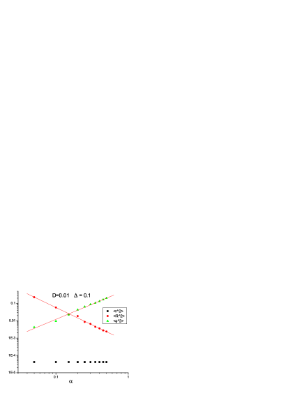
Figure 8: $\langle\phi^{2}\rangle$ (triangles) $\langle r^{2}\rangle$ (squares) and $\langle R^{2}\rangle$ (circles) as a function of $\alpha$, for two coupled oscillators where $\omega=1+\alpha r$, $D=0.01$ and $\Delta=0.1$. Clearly the value of $\langle r^{2}\rangle$ is almost independent of the frequency gradient $\alpha$. $\langle R^{2}\rangle$ is fitted to $\alpha^{-1.99}$, in agreement with Eq. ( 16). $\langle\phi^{2}\rangle$ scales like $\alpha^{1.74}$, close to the prediction of (14).

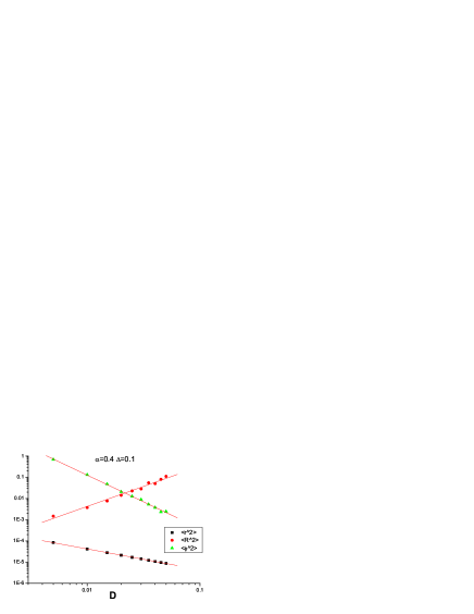
Figure 9: $\langle\phi^{2}\rangle$ (triangles) $\langle r^{2}\rangle$ (squares) and $\langle R^{2}\rangle$ (circles) as a function of the migration rate $D$, for two coupled oscillators where $\omega=1+\alpha r$, $\alpha=0.4$ and $\Delta=0.1$. As predicted, $\langle r^{2}\rangle$ is inversely proportional to $D$ (best fit to $D^{-0.98}$). $\langle R^{2}\rangle$ is fitted to $D^{-1.88}$, [predicted exponent is (-2)] and $\langle\phi^{2}\rangle$ scales like $D^{-2.52}$ (predicted value -3).

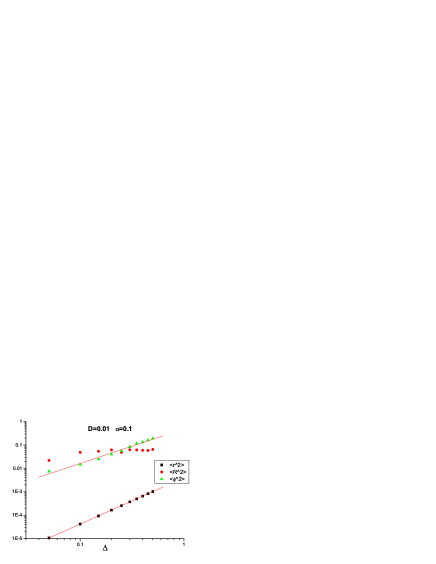
Figure 10: $\langle\phi^{2}\rangle$ (triangles) $\langle r^{2}\rangle$ (squares) and $\langle R^{2}\rangle$ (circles) as a function of the noise $Delta$, for two coupled oscillators where $\omega=1+\alpha r$, $\alpha=0.1$ and $D=0.01$. As predicted, $\langle r^{2}\rangle$ is proportional to $\Delta^{2}$ (best fit to $\Delta^{-1.98}$). $\langle\phi^{2}\rangle$ is fitted to $\Delta^{1.47}$, (predicted exponent is 2) and $\langle R^{2}\rangle$ clearly saturates at large noise levels.

Without the explicit noise term, Eq. (9) may be written as,

$$\dot{\phi}=-2D\left(\frac{R^{2}+r^{2}}{R^{2}-r^{2}}\right)sin\phi-r\frac{\partial\omega}{\partial r}\approx-2D\phi-r\frac{\partial\omega}{\partial r},$$ (13)

where the approximation is valid close to the invariant manifold. Again we face an overdamped harmonic oscillator, where now the source of noise is the $r$ fluctuations (obeying the Boltzman statistics). With that,

$$\langle\phi^{2}\rangle\sim\frac{(\omega^{{}^{\prime}}(r))^{2}\Delta^{2}}{D^{3}},$$ (14)

may be plugged into (7) to yield:

$$\dot{R}=-2Dsin^{2}\left(\frac{\phi}{2}\right)R+\tilde{\eta}_{R}\approx\frac{-D\langle\phi^{2}\rangle R}{2}+\tilde{\eta}_{R}.$$ (15)

Now the ”restoring force” along the R coordinate (the invariant manifold) is finite, and,

$$\langle R^{2}\rangle\sim\frac{D^{2}}{[\omega^{{}^{\prime}}(r)]^{2}}.$$ (16)

This radius of stable oscillations diverges as $D\to\infty$, as expected. The small $D$ instability (decoupled patches) manifest itself in the divergence of $r^{2}$ as $D\to 0$. Surprisingly, since both the restoring force and the noise in the invariant manifold are proportional to $\Delta^{2}$, the expected $R$ distribution has to be noise-independent at that limit, as demonstrated in Figures 7 and 12. A more careful examination of the predictions about the expectation value of the three parameters (Eqs. 16, 14 and the Boltzman distribution for amplitude desynchronization) is presented in Figs. 9, 8, and 10. The small deviations from the predicted exponents are related to the failure of the approximations used far from the invariant manifold. Decreasing the noise level, these exponents approach their predicted values. Figure 11 shows the $D$ dependence of the lifetime for the coupled oscillator model; its agreement with figure 5 is evident.

Figure 11: The typical persistence time as a function of the diffusion rate for different levels of noise for the coupled oscillator model. The ”extinction” was declared when the amplitude of oscillations for one of the patches exceeded unity. The values of $\tau$ were gathered from survival probability plots (like those in Figure 3). One clearly observes the similarity with Figure 5. Data is shown for different noise intensities $\Delta=0.3$ (triangles), $0.4$ (squares) and $0.5$ (circles). Note that while the expectation value of $R^{2}$ is noise independent, the noise still controls the probability to rare fluctuations that leads to extinction.

Another direct manifestation of the coupled oscillator predictions in the LV system is presented in Figure 12. Again, for ”intermediate” migration (e.g., $D=0.01$), the average distance from the origin saturates, while the chance to find the system at large $H$ becomes exponentially small, as illustrated in Figure 12. In agreement with the results of the toy model, the flow toward the center is correlated with the phase desynchronization, leading to stabilization of oscillations at finite $H$. As predicted, while the width of the $\phi^{2}$ distribution depends strongly on the noise amplitude, the oscillation amplitude is almost noise independent.

Figure 12: The average $\Delta H$ at an elementary time step (0.001 of a unit time) as a function of the angle $\phi$ between the patches. While a simple phase space random walk yields, on average, positive $\Delta H$, this property is shown here to hold only for small $\phi$. At larger angles, the diffusion between patches forces the system toward the center and the average $\Delta H$ becomes negative. Results are shown for $\Delta=0.1$ (full line) and $\Delta=1$ (dashed line). The inset shows the probability distribution function for $H$ at these two noise levels.

IV.2 The Coupled oscillators model and NB instability

In order to imitate the behavior of the NB system with its unstable fixed point, Eqs. (IV.1) should be modified to include this new ingredient, manifested here by the terms proportional to $\kappa$,

$$\frac{\partial x_{1}}{\partial t} = \kappa x_{1}+\omega(x_{1},y_{1})y_{1}+D_{1}(x_{2}-x_{1})+\eta_{1}(t)$$

$$\frac{\partial x_{2}}{\partial t} = \kappa x_{2}+\omega(x_{2},y_{2})y_{2}+D_{1}(x_{1}-x_{2})+\eta_{2}(t)$$

$$\frac{\partial y_{1}}{\partial t} = \kappa y_{1}-\omega(x_{1},y_{1})x_{1}+D_{2}(y_{2}-y_{1})+\eta_{3}(t)$$ (17)

$$\frac{\partial y_{2}}{\partial t} = \kappa y_{2}-\omega(x_{2},y_{2})x_{2}+D_{2}(y_{1}-y_{2})+\eta_{4}(t).$$

The system is still invariant with respect to global rotation, thus it reduces to the three dimensional phase space:

$$\dot{R} = \left(\kappa-2Dsin^{2}(\phi/2)\right)R+\tilde{\eta}_{R}$$ (18)

$$\dot{r} = \left(\kappa-2Dcos^{2}(\phi/2)\right)r+\tilde{\eta}_{r}$$ (19)

$$\dot{\phi}=-2 D \left(\frac{R^{2}+r^{2}}{R^{2}-r^{2}}\right)sin\phi+\omega(r_{2})-\omega(r_{1})+\left(\frac{\tilde{\eta}_{1}}{r_{1}}-\frac{\tilde{\eta}_{2}}{r_{2}}\right).$$ (20)

Close to the invariant manifold, thus,

$$P(r)\sim exp[-(2D-\kappa))r^{2}/\Delta^{2}]$$ (21)

and

$$\langle\phi^{2}\rangle\sim\frac{\omega^{{}^{\prime}}(r)^{2}\Delta^{2}}{D(2D-\kappa)^{2}}.$$ (22)

Consequently:

$$\langle R^{2}\rangle\sim\frac{\Delta^{2}}{D\langle\phi^{2}\rangle-\kappa}=\frac{\Delta^{2}}{\omega^{{}^{\prime}}(r)^{2}\Delta^{2}/(2D-\kappa)^{2}-\kappa}.$$ (23)

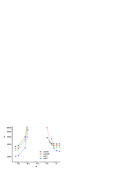
Figure 13: Extinction times for the unstable, coupled oscillator cartoon of the Nicholson-Bailey model. Eqs. (IV.2) were integrated numerically (using Euler integration with $\Delta t=0.002$) for $\kappa=0.0001$ and and $\omega=\omega_{0}+r/2$ for different noise amplitudes $\Delta$ and diffusion constant D. The extinction time is plotted for four different noise level against the diffusion constant, and the two transitions are implicit. The lifetime of the system for large noise ($\Delta=0.1,0.2$, triangles) diverges beyond our computational abilities for $D=0.01$.

The system becomes unstable when either $r^{2}$ or $R^{2}$ diverge. The first criterion for stability comes from the amplitude synchronization parameter, $2D>\kappa$, so the diffusion should increase above some threshold value in order to prevent desynchronized extinction where the system acts as if made of two disconnected patches. As in the LV case, if the migration rate is too large (i.e., if $\kappa$ becomes larger than $[\omega^{{}^{\prime}}(r)]^{2}\Delta^{2}/(2D-\kappa)^{2}\sim\omega^{\prime 2}\ \Delta^{2}/D^{2}$), the system synchronizes and the deterministic flow leads to synchronized extinction. Note that close to the low D transition the extinction rate grows with the noise, while close to the second transition, increase of noise amplitude $\Delta$ yields lower extinction rates, emphasizing the fact that the stability is noise-induced. This feature is clearly seen in Figure 14, where for small noise the oscillation amplitude grows exponentially in time while for large noise the oscillation stabilizes.

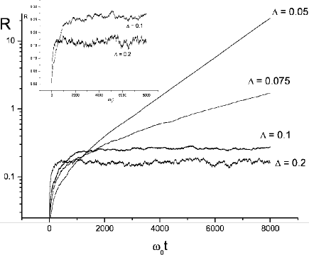
Figure 14: Noise-induced transition for the coupled oscillator cartoon of the Nicholson-Bailey model. Eqs. (IV.2) were integrated numerically (using Euler integration with $\Delta t=0.002$) with $\kappa=0.0001$, $D=0.01$ and $\omega=\omega_{0}+r/2$ for different noise amplitudes $\Delta$. The total distance $R$ (averaged over 100 runs) is presented, in logarithmic scale, against time measured in units of $\omega_{0}$. Small noises are followed by exponential growth of the oscillation amplitude, as suggested by the deterministic part of (IV.2). The larger the noise, the slope of this diverging line becomes smaller. If the noise is large enough, $R$ saturates at a finite value, as seen more clearly when the scale is not logarithmic (inset).

Along this section, the various numerical implementation of the toy assumes, for simplicity, that the oscillation frequency depends linearly on the slope. If, on the other hand, $\omega^{\prime}$ is a nonuniform function of the amplitude, oscillations will grow sublinearly (for the LV model) or exponentially (in NB case) with time, until they reach a phase space region where $\partial\omega/\partial r$ is large enough. For an LV-like system it leads to the appearance of a ”soft” limit cycle - exponential convergence from the outside, diffusion inside.

It should be noted that the stability mechanism presented here is applicable not only for the classic predator-prey systems but for any biological system that supports, locally, neutrally stable or unstable oscillations. In particular it may stabilize a ”locally” unstable ecology of interspecific competition for common resource. Such a system may be described mathematically by the generalized Lotka-Volterra equations (Chesson, 2000); even if the theory predicts extinction, species diversity may be maintained on spatial domains. Another possible application is the stabilization of ”eigenperiods” - oscillations due to the interaction between an individual and its internal resources or by maternal effect - suggested recently as a predation free mechanism for population oscillations (Ginzburg and Colyvan, 2004).

V Other Mechanisms

This section is devoted to a discussion of previously suggested stabilization mechanisms in the framework of the coupled oscillator toy model. We show that all the significant mechanisms surveyed by (Briggs and Hoopes , 2004) become very clear and allow analytical understanding when presented using the coupled oscillator system.

V.1 Spatial heterogeneity

To implement the spatial heterogeneity (SH) (Murdoch and Oaten , 1975; Murdoch et al, 1992; Hassell and May, 1988) in our framework, consider a two patch system with different (radius independent) frequencies, $\omega_{1}$ and $\omega_{2}$:

$$\frac{\partial x_{1}}{\partial t} = \omega_{1}y_{1}+D_{1}(x_{2}-x_{1})+\eta_{1}(t)$$

$$\frac{\partial x_{2}}{\partial t} = \omega_{2}y_{2}+D_{1}(x_{1}-x_{2})+\eta_{2}(t)$$

$$\frac{\partial y_{1}}{\partial t} = -\omega_{1}x_{1}+D_{2}(y_{2}-y_{1})+\eta_{3}(t)$$ (24)

$$\frac{\partial y_{2}}{\partial t} = -\omega_{2}x_{2}+D_{2}(y_{1}-y_{2})+\eta_{4}(t).$$

As these equations are linear, one may again diagonalize the deterministic part of the evolution matrix to obtain the exact probability distribution function. However, as this problem is still invariant under global rotation and is independent of $\theta_{1}+\theta_{2}$ we have chosen to use the more intuitive polar representation. After the standard coordinates transformation, one finds:

$$\dot{R} = -2Dsin^{2}\left(\frac{\phi}{2}\right)R+\tilde{\eta}_{R}$$ (25)

$$\dot{r} = -2Dcos^{2}\left(\frac{\phi}{2}\right)r+\tilde{\eta}_{r}$$ (26)

$$\dot{\phi}=-2 D \left(\frac{R^{2}+r^{2}}{R^{2}-r^{2}}\right)sin\phi+[\omega_{2}-\omega_{1}]+\left(\frac{\tilde{\eta}_{1}}{r_{1}}-\frac{\tilde{\eta}_{2}}{r_{2}}\right).$$ (27)

Here $\Delta\omega\equiv\omega_{2}-\omega_{1}$ is a constant, so close to the invariant manifold, $r$ decouples from $\phi$. Consequently, while $P(r)$ is still given by 12, $\phi$ satisfies an equation for a forced overdamped pendulum and $sin(\phi)=\Delta\omega/2D$. The ”spring constant” in the invariant manifold $R$ is thus noise-independent and

$$\langle R^{2}\rangle\sim\frac{D\Delta^{2}}{(\Delta\omega)^{2}}.$$ (28)

The radius of oscillation in a heterogenous system increases with noise: the system becomes more extinction prone as the noise grows larger. In the corresponding ”Nicholson-Bailey” toy model the phase transition happens at $\kappa=D/(\Delta\omega)^{2}$, and the location of that transition is noise-independent.

V.2 Environmental stochasticity

The above framework may also be used to consider the stabilizing effect of spatio-temporal environmental stochastisity (STES) (Crowley, 1981; Reeve, 1990; Taylor, 1998). If on both patches the radial velocity takes the form $\omega+\zeta_{i}(t)$, where $i$ is the patch index and $\zeta$ is a white noise that satisfies $\langle\zeta(t)\zeta(t^{\prime})\rangle=\Upsilon\delta(t-t^{\prime})$, the $\phi$ variable obeys an equation for an overdamped noisy pendulum and the resulting motion on the invariant manifold satisfies:

$$\dot{R}=\left(\kappa-\Upsilon\right)R+\eta_{R},$$ (29)

so $\langle R^{2}\rangle\sim\Delta^{2}/(\Upsilon-\kappa)$. In that case the lifetime of the system is diffusion-independent, growing with the environmental stochasticity and decaying with the noise.

V.3 Jansen instability

About ten years ago, Jansen (Jansen, 1995; Jansen and de Roos, 2000; Jansen and Sigmund, 1998) put forward the idea of linearly unstable orbits of the Lotka-Volterra dynamics, i.e., orbits in the homogenous manifold for which the highest absolute value of an eigenvalue of the Floquet operator is larger than 1. This may happen only if the migration properties of the prey and the predator are different. In the case of equal diffusivities, the migration term factors out from the Floquet operator and the stability properties of orbits lying in the invariant manifold are the same as their matching trajectories on a single patch (Abarbanel, 1995). However, Jansen pointed out that if one sets $D_{b}=0$ in Eqs. IV, some orbits may become unstable. In that case one may use the fact that the total $H$

$$\ H_{T}\equiv H_{1}+H_{2}=a_{1}+a_{2}+b_{1}+b_{2}-ln(a_{1}a_{2}b_{1}b_{2}),$$ (30)

with the deterministic dynamics (IV) is a monotonously decreasing quantity in the non negative population regime:

$$\frac{dH_{T}}{dt}=-D_{a}\left(\frac{(a_{1}-a_{2})^{2}}{a_{1}a_{2}}\right)-D_{b}\left(\frac{(b_{1}-b_{2})^{2}}{b_{1}b_{2}}\right)<0.$$ (31)

Accordingly, if an orbit on the invariant manifold becomes unstable, the flow will be inward and the population oscillations stabilize.

With the transformation,

$$A=\frac{a_{1}+a_{2}}{2}\qquad B=\frac{b_{1}+b_{2}}{2}$$ (32)

$$\delta=\frac{a_{1}-a_{2}}{2}\qquad\theta=\frac{b_{1}-b_{2}}{2},$$

one realizes the homogenous $AB$ manifold and the $\delta-\theta$ coordinates that measures the deviation from that manifold (the heterogeneity of the population). In these coordinates the system satisfies,

$$\frac{\partial A}{\partial t} = -\mu A+\lambda_{1}AB+\lambda_{1}\delta\theta$$ (33)

$$\frac{\partial B}{\partial t} = \sigma B-\lambda_{2}AB+\lambda_{2}\delta\theta$$

$$\frac{\partial\delta}{\partial t} = -\mu\delta+\lambda_{1}A\theta+\lambda_{1}B\delta-2D_{a}\delta$$

$$\frac{\partial\theta}{\partial t} = \sigma B-\lambda_{2}A\theta-\lambda_{2}B\delta-2D_{b}\theta.$$

Linearizing around the homogenous manifold, the $AB$ dynamic is equivalent to that of a single patch,

$$\dot{A} = -\mu A+\lambda_{1}AB$$ (34)

$$\dot{B} = \sigma B-\lambda_{2}AB$$

and the $\delta-\theta$ linearized dynamic is

$$\frac{\partial}{\partial t}\left(\begin{array}[]{cc}\delta\\ \theta\\ \end{array}\right)=\left(\begin{array}[]{cc}-\mu+\lambda_{2}A-2D_{a}&\lambda_{2}\\ -\lambda_{2}A&\sigma-\lambda_{2}B-2D_{b}\\ \end{array}\right)\left(\begin{array}[]{cc}\delta\\ \theta\\ \end{array}\right).$$ (41)

One may thus calculate the eigenvalues of the Floquet operator for one period along an orbit of (34). The resulting stability diagram, first obtained by (Jansen, 1995), is shown in Figure 15.

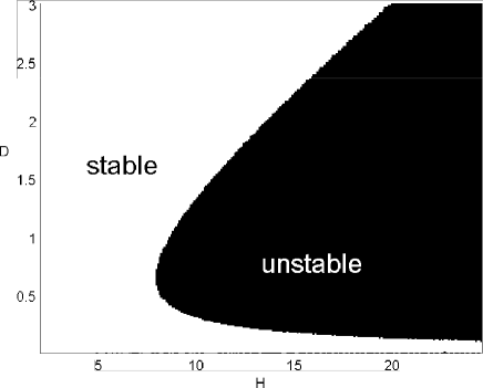
Figure 15: Stability diagram for phase space orbits (ordered by their conserved quantity $H$) for different values of predator diffusion $D_{a}$, where Db=0.

We have discussed Jansen’s stabilization mechanism in a different publication (Abta and Shnerb, 2006b). It turns out that the underlying mechanism has to do with the dependence of the angular velocity along the orbit on the azimuthal angle (see Figure 6), and we can mimic that behavior using our toy model with $\omega(\theta)$. Specifically, the coupled oscillator model with,

$$\frac{\partial x_{1}}{\partial t} = \omega(\theta_{1})y_{1}+D_{x}(x_{2}-x_{1})$$ (42)

$$\frac{\partial x_{2}}{\partial t} = \omega(\theta_{2})y_{2}+D_{x}(x_{1}-x_{2})$$

$$\frac{\partial y_{1}}{\partial t} = -\omega(\theta_{1})x_{1}+D_{y}(y_{2}-y_{1})$$

$$\frac{\partial y_{2}}{\partial t} = -\omega(\theta_{2})x_{2}+D_{y}(y_{1}-y_{2}),$$

where $D_{x}=D,\ D_{y}=0$ and

$$\omega = \omega_{0}+\omega_{1}\cos(\theta-\frac{\pi}{4}),$$ (43)

leads to the same type of instability.

To prove that this model actually yields Jansen’s instability, we have used ($i\in 1,2$)

$$r_{i}^{2}=x_{i}^{2}+y_{i}^{2} \theta_{i}=arctan(\frac{y_{i}}{x_{i}})$$ (44)

$$\dot{r}=\frac{(x\dot{x}+y\dot{y})}{r} \dot{\theta}=\frac{(x\dot{y}-y\dot{x})}{r^{2}},$$

and

$$r=r_{2}-r_{1} R=r_{2}+r_{1}$$ (45)

$$\phi=\theta_{2}-\theta_{1} \Phi=\theta_{2}+\theta_{1}.$$

The flow in the invariant manifold satisfies,

$$\dot{R} = 0$$ (46)

$$\dot{\Phi} = \omega(\theta_{1})+\omega(\theta_{2}),$$

while the linearized equations for the desynchronization amplitude $r$ and the desynchronization angle $\phi$ satisfy:

$$\frac{\partial}{\partial t}\left(\begin{array}[]{cc}\phi\\ r\\ \end{array}\right)=\left(\begin{array}[]{cc}2\omega^{\prime}(\Phi/2)-4D_{x}\cos^{2}(\Phi/2)&\frac{2D_{x}\sin\Phi}{R}\\ -D_{x}R\sin(\Phi)&-4D_{x}\sin^{2}(\Phi/2)\\ \end{array}\right)\left(\begin{array}[]{cc}\phi\\ r\\ \end{array}\right).$$ (53)

Using the Floquet operator technique to analyze the stability of an orbit by integrating (53) along a close trajectory of (46), one finds the stability map presented in Figure 16, where the parameter $H$ of Figure 15 is now replaced by $\omega_{1}$, which measures the ”eccentricity” of the angular velocity along a circular path. Here, two unstable regions appear, for large and small $D_{x}$, but the qualitative picture is almost the same.

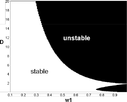
Figure 16: Stability diagram in the $\omega_{1}-D_{x}$ plane for the Floquet operator (same as Figure 15) for the coupled oscillator system described by Eqs. (42) with $D_{y}=0$. The two unstable regions correspond to different signs of the Floquet unstable eigenvalue, as explained in the text.

VI Concluding remarks: Towards classification of sustained oscillations.

Up until now, four different mechanisms that induce stability of population oscillations for metapopulations have been presented. The generic mechanism relies on the dependence of the oscillation frequency on their amplitude (ADF, Amplitude Dependent Frequency). The other three are spatial heterogeneity (SH), spatio-temporal environmental stochasticity (STES), and Jansen’s mechanism based on the dependence of the angular velocity on the azimuthal angle.

In natural systems, in the laboratory, and in simulations, one may encounter population oscillations in the presence of a few of the above mentioned factors, simultaneously. The task of the researcher is to make a distinction between them and to identify the relevant, or the most relevant, stabilizing mechanism. To do that, the following comments may be useful:

• Some of the parameters involved, such as the migration rate per capita, the strength of the environmental stochasticity, growth and competition parameters and so on, may be known from the literature or may be measured independently. If possible, an estimate of the stable oscillation amplitude has to be made and a comparison between possible mechanisms will reveal the dominant one, which is (in the long run) the one that stabilizes the smallest oscillation amplitude.

• If the dominant mechanism is spatial heterogeneity, the phase between cycles on neighboring patches is kept constant in time. Thus, it is quite easy to recognize an SH-induced stability. In all other cases there is no preference among patches and $\phi$ is distributed randomly around zero.

• Jansen’s RVA instability depends very much on the difference between species diffusivities. It is impossible to observe such an instability in host-parasite systems, where the parasite migration depends on host movement.

• One way to distinguish between STES and ADF is to separately manipulate the additive noise (taking small portions of the population in and out of the system at random) and environmental stochasticity. An increase in the amplitude $\Delta$ of the additive noise leads to larger oscillations for STES and smaller/equal oscillation amplitudes for ADF; amplified stochasticity will diminish oscillations if the basic mechanism is STES, and is neutral in ADF-controlled systems. Another test is the response of the system to changes in the migration rate, where STES synchronized oscillation amplitudes are not affected by changes in $D$.

• In both SH and STES mechanisms, the amplitude desynchronization decouples from the phase desynchronization, while in ADF they are intimately connected. Measurements of the correlations between the phase and the amplitude desynchronization will immediately reveal the relevant mechanism.

As pointed out by Jansen and Sigmund (Jansen and Sigmund, 1998), ”all models of ecological communities are approximations: it is pointless to burden them with too many contingencies and details. On the other hand, they would be of little help if they were not robust against the kind of perturbation and shocks to which a real ecosystem is ceaselessly exposed.” The current accuracy of data on population oscillations and inter-specific interaction, both from field studies and from experiments, is, as far as we know, far beyond the level needed for an exact comparison with theoretical predictions about the oscillation phase portrait, like those predicted by Lotka-Volterra and other models. Given that, the main insights from the available data are, first, the mere existence of these oscillations, and second, the identification of the underlying mechanism that limits the amplitude of these oscillations in noisy environments. As emphasized by the recent experiments of (Kerr et al., 2002 ; Kerr et al., 2006) , one may observe persistent oscillations or extinction, but it is hard to compare the exact population dynamic with the predictions of the theory. Accordingly, the analysis of data on population cycles may be preformed, as we have shown here, completely within the framework of the simple coupled oscillation model that allows all the suggested limiting processes within a transparent and general modeling scheme.

VII Acknowledgements

We acknowledge helpful discussions with David Kessler, Uwe T$\ddot{\textrm{a}}$uber, and Arkady Pikovsky. This work was supported by the Israeli Science Foundation (grant no. 281/03) and the EU 6th framework CO3 pathfinder.

REFERENCES

• Abarbanel H.D.I., 1995. Analysis of observed chaotic data Springer, Berlin, p. 87.

• Abta R., Schiffer M. and Shnerb M.N., 2006a, Amplitude dependent frequency, desynchronization, and stabilization in noisy metapopulation. dynamics. cond-mat/0608108.

• Abta R. and Shnerb M.N., 2006b. Angular velocity variations and stability of spatially explicit prey-predator systems. q-bio.PE/0612021.

• Allen, J.C., 1975. Mathematical models of species interactions in space and time. Am. Nat. 109, 319 342.

• Bettelheim E., Agam O. & Shnerb N.M., 2000. ”Quantum phase transitions”” in classical nonequilibrium processes, Physica E 9, 600-608.

• Blasius B., Huppert A. & Stone L., 1999. Complex dynamics and phase synchronization in spatially extended ecological systems. Nature 399, 354-359.

• Briggs C.J. & Hoopes M.F., 2004. Stabilizing effects in spatial parasitoid host and predator prey models: a review. Theoretical Population Biology 65, 299-315.

• Chesson P., 2000. Mechanisms of maintenance of spatial diversity. Annu. Rev. Ecol. Syst. 31, 343-366.

• Crowley, P.H., 1981. Dispersal and the stability of predator prey interactions. Am. Nat. 118, 673 701.

• Cuddington K., 2001. The ”balance of nature” metaphor and equilibrium in population ecology. Biology and Philosophy 16, 463-479.

• Earn D.J.D., Levin S.A. & Rohani P., 2000. Coherence and Conservation. Science 290, 1360-1363.

• Elton C.S., 1924. Periodic Fluctuations in the Numbers of Animals: Their Causes and Effects. Br. Jour. Exp. Biol. 2; 119-163.

• Foley P., 1997. extinction models for local population, in Metapopulation Biology - Ecology, Genetics ana Evolution, I.A. Hanski and M.E. Gilpin (Ed.) Academic Press (London).

• Freeman D.B., 1992. Prickly pear menace in eastern Australia 1880-1940. Geographical Review 82, 413-429.

• Gardiner C.W., 2004. Handbook of Stochastic Methods, Springer, Berlin.

• Gause G.F., 1934. The struggle for existence. William and Wilkins, Baltimore.

• Gillespie D.T., 1977. Exact stochastic simulation of coupled chemical reactions . Journal of Physical Chemistry, 81, 2340-2361.

• Ginzburg L. and Colyvan M., 2004. Ecological Orbits, Oxford University Press, Oxford U.K.

• Grassberger. P., 1982. On phase transitions in Schlogl’s model. Z. Phys. B: Condens. Matter 47, 365-374.

• Grimm V. and Wissel C., 2004. The intrinsic mean time to extinction: a unifying approach to analysing persistence and viability of populations. Oikos 105, 501-511.

• Hassell, M.P., May R.M., 1988. Spatial heterogeneity and the dynamics of parasitoid host systems. Ann. Zool. Fenn. 25, 55 62.

• Hassell, M.P., Varley, G.C., 1969. New inductive population model for insect parasites and its bearing on biological control. Nature 223, 1133 1137.

• Holyoak M. & Lawler S.P., 1996. Persistence of an Extinction-Prone Predator-Prey Interaction Through Metapopulation Dynamics. Ecology 77, 1867-1879.

• Huffaker C.B., 1958. Experimental studies on predation: dispersion factors and predator prey oscillations. Hilgardia 27 343-383.

• Jansen, V.A.A., 1995. Regulation of predator prey systems through spatial interactions: a possible solution to the paradox of enrichment. Oikos 74, 384-390.

• Jansen V.A.A and de Roos A.M., 2000. In: The Geometry of Ecological Interactions: Simplifying Spatial Complexity, eds. Dieckmann U., Law R and Metz J.A.J., pp. 183 Cambridge University Press.

• Jansen V.A.A. and Sigmund K., 1998. Shaken Not Stirred: On Permanence in Ecological Communities. Theo. Pop. Bio. 54, 195-201.

• Janssen H.K., 1981. On the nonequilibrium phase transition in reaction-diffusion systems with an absorbing stationary state. Z. Physik. 42, 151-154.

• Kerr B., Neuhauser C., Bohannan B.J.M. & Dean A.M., 2006. Local migration promotes competitive restraint in a host-pathogen ’tragedy of the commons’. Nature 442, 75-78.

• Kerr B., Riley M.A., Feldman M.W. and Bohannan B.J.M., 2002. Local dispersal promotes biodiversity in a real-life game of rock-paper-scissors. Nature 418, 171-174.

• Kessler D.A. and Shnerb M.N., 2006. Extinction Rates for Fluctuation-Induced Metastabilities: A Real-Space WKB Approach. q-bio.PE/0611049.

• Kirkup B.C. and Riley M.A., 2004. Antibiotic-mediated antagonism leads to a bacterial game of rock-paper-scissors in vivo. Nature 428 412-414

• Kolmogorov A., 1936. Sulla teoria di Volterra della lotta per l’esistenze. G. Ins. Ital. Attnari 7 985-992.

• Lande R., Engen S. and Saether B.E., 2003. Stochastic Population Dynamics in Ecology and Conservation, Oxford University Press, Oxford U.K.

• Lotka A.J. 1920. Analytical note on certain rhythmic relations in organic systems. Proc. Natl. Acad. Sci. USA 6, 410-415.

• Luckinbill L.S., 1974. The Effects of Space and Enrichment on a Predator-Prey System. Ecology, 1142-1147.

• May R.M., 1972. Limit cycles in predator prey communities. Science 177 900-902.

• May, R.M.,1978. Host-parasitoid systems in patchy environments: a phenomenological model. J. Anim. Ecol. 47, 833-843.

• Mobilia M., Georgiev I.T. and Tauber U.C., 2006. Fluctuations and Correlations in Lattice Models for Predator-Prey Interaction. Phys. Rev. E 73, 040903.

• Murdoch, W.W., Briggs, C.J., Nisbet, R.M., Gurney, W.S.C., Stewart- Oaten, A., 1992. Aggregation and stability in metapopulation models. Am. Nat. 140, 41 58.

• Murdoch, W.W., Oaten, A., 1975. Predation and population stability. Adv. Ecol. Res. 9, 1 131.

• Murray J.D.,1993 Mathematical Biology. (Springer-Verlag, New-York).

• Nicholson, A.J., 1933. The balance of animal populations. J. Anim. Ecol. 2, 132-178.

• Nicholson, A.J., Bailey, V.A. 1935. The balance of animal populations Proc. Zool. Soc. London Part I 3, 551-598.

• Pimentel D., Nagel W.P. & Madden J.L., 1963. Space-time structure of the environment and the survival of parasite-host systems American Naturalist, 97, 141-167.

• Reeve, J.D., 1990. Stability, variability, and persistence in host parasitoid systems. Ecology 71, 422 426.

• Redner S., 2001. A Guide to First-Passage Processes, Cambridge University Press, Cambridge.

• Reichenbach T., Mobilia M. and Frey E., 2006. Coexistence versus extinction in the stochastic cyclic Lotka-Volterra model. Phys. Rev. E 74, 051907.

• Rosenzweig, M.L., MacArthur, R.H., 1963. Graphical representation and stability conditions of predator prey interactions. Am. Nat. 97, 209 223.

• Stenseth et. al., 1998. From patterns to processes: Phase and density dependencies in the Canadian lynx cycle. Proc. Natl. Acad. Sci. USA 95, 15430-15435.

• Taylor A.D., 1990. Metapopulations, Dispersal, and Predator-Prey Dynamics: An Overview. Ecology 71, 429-433.

• Taylor A.D., 1998. Environmental variability and the persistence of parasitoid host metapopulation models. Theo. Pop. Biol. 53, 98-107.

• Volterra V, 1931. Lecon sur la Theorie Mathematique de la Lutte pour le via, Gauthier-Villars, Paris.

• Washenberger M.J., Mobilia M. & T$\rm{\ddot{a}}$uber U.C., 2006. Influence of local carrying capacity restrictions on stochastic predator-prey models. cond-mat/0606809.

• Wilmers C.C, Post E., Peterson R.O. & Vucetich J.A, 2006. Predator disease out-break modulates top-down, bottom-up and climatic effects on herbivore population dynamics. Ecology Letters, 9 383 389.

• Wilson, W.G., de Roos, A.M., McCauley, E., 1993. Spatial instabilities within the diffusive Lotka Volterra system: individual-based simulation results. Theor. Popul. Biol. 43, 91 127.