Quantitative Protein Dynamics from Dominant Folding Pathways

Abstract

We develop a theoretical approach to the protein folding problem based on out-of-equilibrium stochastic dynamics. Within this framework, the computational difficulties related to the existence of large time scale gaps in the protein folding problem are removed and simulating the entire reaction in atomistic details using existing computers becomes feasible. In addition, this formalism provides a natural framework to investigate the relationships between thermodynamical and kinetic aspects of the folding. For example, it is possible to show that, in order to have a large probability to remain unchanged under Langevin diffusion, the native state has to be characterized by a small conformational entropy. We discuss how to determine the most probable folding pathway, to identify configurations representative of the transition state and to compute the most probable transition time. We perform an illustrative application of these ideas, studying the conformational evolution of alanine di-peptide, within an all-atom model based on the empiric GROMOS96 force field.

A critical part of the protein-folding problem is to understand its kinetics and the underlying physical processes. To this aim, several different theoretical methods have been recently developed, spanning from analytical approachesTheoAdv1 ; TheoAdv2 ; TheoAdv3 to detailed computer simulationsSimAdv1 ; SimAdv2 ; SimAdv3 . A major problem in simulating the folding process using standard molecular dynamics (MD) is the huge gap between the time scale of “elementary moves”, of the order of 10-100 ps, and that of the entire folding process, which ranges from a few microseconds for fast-foldersFastFolders , up to several seconds or even minutes for more complex proteins. This peculiarity of the folding process makes the brute-force molecular dynamics approach too demanding, and a substantial part of the efforts in the field of protein folding simulation aims at bridging this gap.

In a recent paper DFP we have presented a novel theoretical framework for investigating the folding dynamics, named hereafter Dominant Folding Pathways (DFP), which is based on a reformulation in terms of path integrals of the dynamics described by the Langevin equation. The DFP analysis allows to compute rigorously (i.e. without any assumptions other than the validity of the underlying Langevin equation) the most probable conformational pathway connecting an arbitrary initial conformation to an arbitrary final conformation. The major advantage of the method is the possibility of bypassing the computational difficulties associated with the existence of different time scales in the problem, while retaining the ability to recover information on the time evolution of the system. As we shall see, the resulting computational simplification is dramatic and makes it feasible to study the formation pattern of conformational structures along the entire folding process using realistic all-atom force fields, on available computers.

In this Letter we further develop our formalism and we present the first DFP simulation performed in full atomistic detail. We show how the DFP analysis gives access to important information about the dynamics of the folding process, such as the characterization and determination of the transition state, and the most probable transition time. In addition, we show that in this formalism the native state is characterized by a single effective parameter and this leads to an interesting relationship between kinetic and thermodynamical quantities.

Let us begin our discussion by briefly reviewing the key concepts of the DFP method, here presented for a simple one-dimensional system, without loss of generality.

The DFP method can be applied to any system described by the over-damped Langevin equation

$$\frac{\partial x}{\partial t}=-\frac{D}{k_{B}T}\frac{\partial U}{\partial x}+\eta(t),$$ (1)

where $U$ is the potential energy of the system, $\eta(t)$ is a Gaussian random force with zero average and correlation given by $\langle\eta(t)\eta(t^{\prime})\rangle=2D\delta(t-t^{\prime})$. Note that in the original Langevin equation there is a mass term, $m\ddot{x}$. However, as shown in Pitard , for proteins, this term can be neglected beyond time scales of the order of $10^{-13}$ s.

The probability of finding the system in a conformation $x_{f}$ at time $t_{f}$ starting from a conformation $x_{i}$ at $t_{i}$, is a solution of the well-known Fokker-Planck Equation, and can be expressed as a path-integral:

$$P(x_{f},t_{f}|x_{i},t_{i})=e^{-\frac{U(x_{f})-U(x_{i})}{2k_{B}T}}\int_{x_{i}}^{x_{f}}\mathcal{D}x(\tau)\,e^{-{S_{eff}[x]}},$$ (2)

where

$$S_{eff}[x]=\int_{t_{i}}^{t_{f}}d\,\tau~{}\left(\frac{\dot{x}^{2}(\tau)}{4D}+V_{eff}[x(\tau)]\right),$$ (3)

is called the effective action and

$$V_{eff}(x)=\frac{D}{4(k_{B}T)^{2}}\,\left[\left(\frac{\partial U(x)}{\partial x}\right)^{2}-2k_{B}T\frac{\partial^{2}~{}U(x)}{\partial x^{2}}\right].$$ (4)

is called the effective potential. This quantity measures the tendency of a configuration to evolve under Langevin diffusion. In fact, the probability for the system to remain in the same configuration $x$ under an infinitesimal time interval is given by

$$P(x,dt|x,0)=e^{-V_{eff}(x)dt}$$ (5)

Hence, points of large effective potential are highly unstable under Langevin diffusion.

There is an obvious sum rule: $\int dx_{f}P(x_{f},t_{f}|x_{i},t_{i})=1$, which can be written as

$$1=e^{\frac{U(x_{i})}{2k_{B}T}}\int dx_{f}~{}\int_{x_{i}}^{x_{f}}\mathcal{D}x(\tau)\,e^{-\frac{U(x_{f})}{2k_{B}T}-{S_{eff}[x]}}$$ (6)

>From a saddle-point analysis of this sum-rule, it follows that given the initial condition $(x_{i},t_{i})$, the most probable paths contributing to (6) satisfy the Euler-Lagrange equations derived from the effective Lagrangian $L_{eff}=\dot{x}^{2}/4D+V_{eff}(x)$ with proper boundary conditions

$$\frac{d^{2}x}{dt^{2}} = 2D\frac{\partial V_{eff}}{\partial x}$$ (7)

$$\dot{x}_{f} = -\frac{D}{k_{B}T}U^{\prime}(x_{f})$$ (8)

$$x(t_{i}) = x_{i}$$ (9)

The saddle-point equation (8), which comes from the variation of the exponent in (6) with respect to the final point $x_{f}$, tells us which final points dominantly contribute to the sum rule, that is which conformations are most likely to be visited at the final time, $t_{f}$.

The numerical advantage in determining the DFP comes from the fact that $L_{eff}$ is a Lagrangian describing an energy conserving dynamics, and therefore it is possible to use the Hamilton-Jacobi (HJ) description. With this change of framework, the total computational cost of the simulation now depends on the length of the path, rather than on the folding time. In the HJ framework, the most probable pathway is obtained by minimizing — not just extremizing — the functional

$$S_{HJ}([x];x_{i},x_{f})=~{}\int_{x_{i}}^{x_{f}}dl\sqrt{1/D\left(E_{eff}+V_{eff}[x(l)]\right)},$$ (10)

where $dl=\sqrt{(dx)^{2}}$ is an infinitesimal conformational change along the path and the effective energy is given by

$$E_{eff}=\frac{\dot{x^{2}}}{4D}-V_{eff}(x).$$ (11)

Since the effective energy is conserved along the DFP, using equation (8) we have

$$E_{eff}=\frac{D}{2k_{B}T}U^{\prime\prime}(x_{f}).$$ (12)

Note that, since the diffusion coefficient drops exponentially at low temperatures, $D=D(T)\sim D_{0}\exp[-E_{a}/k_{B}T]$, the effective energy vanishes in this limit. In the long time limit, $t_{f}\to\infty$, we know that $P(x_{f},t_{f}|x_{i},t_{i})$ converges to the Boltzmann distribution

$$P(x_{f},t_{f}|x_{i},t_{i})\to_{t_{f}\to\infty}\frac{e^{-U(x_{f})/k_{B}T}}{Z}$$ (13)

where $Z$ is the partition function of the system. If the reaction takes place at a temperature below the folding temperature, at large times the system will sample configurations $x_{f}$ close to the global minimum-potential-energy configuration $x_{n}$, for which $U^{\prime}(x_{n})=0$.

We shall define the native state as the region of configuration space which is thermally accessible from the minimum-energy conformation $x_{n}$, i.e. for which energy differences with respect to $U(x_{n})$ are of the order of $k_{B}T$. We can assume that, for all configurations $x_{f}$ in the native state, the potential energy can be described in the harmonic approximation:

$$U(x_{f})\approx U(x_{n})+\frac{1}{2}U^{\prime\prime}(x_{n})(x_{f}-x_{n})^{2}$$ (14)

This equation together with equation (12) implies

$$E_{eff}=\frac{D(T)}{2k_{B}T}U^{\prime\prime}(x_{n})=-V_{eff}(x_{n})$$ (15)

This equation is quite powerful, since it shows that the effective energy does not depend on the specific conformation $x_{f}$ in the native state, and is totally determined by the temperature of the heat-bath and by the curvature of the potential energy at the minimum-energy point $x_{n}$. Stated differently, the native state belong to a surface in configuration space of constant effective energy $E_{eff}$.

This parameter appears in the macroscopic quantities characterizing the thermodynamics of the native state. As an example, let us discuss the conformational entropy $S_{conf}$, which measures the number of micro-states in the native state, i.e. the contribution to the partition function of all the configurations for which $U(x)-U(x_{n})\lesssim k_{B}T$, where $x_{n}$ is the minimum-energy configuration:

$$Z_{N}(T) = \int dxe^{-\frac{U(x)}{k_{B}T}}~{}\theta\left(k_{B}T-(U(x)-U(x_{n}))\right)$$ (16)

$$S_{conf}(T) \equiv -\frac{\partial}{\partial T}k_{B}T\ln Z_{N}(T)$$ (17)

Expanding the potential energy quadratically around the minimum-energy configuration $x_{n}$ we have

$$Z_{N} \simeq e^{-\frac{U(x_{n})}{k_{B}T}}~{}\int^{x_{n}+\sqrt{2k_{B}T/U^{\prime\prime}(x_{n})}}_{x_{n}-\sqrt{2k_{B}T/U^{\prime\prime}(x_{n})}}dx~{}e^{-\frac{U^{\prime\prime}(x_{n})}{2k_{B}T}(x-x_{n})^{2}},$$ (18)

which gives

$$S_{conf}(T) \simeq k_{B}\ln\left[\sqrt{\frac{2\pi k_{B}T}{U^{\prime\prime}(x_{n})}}~{}\textrm{Erf}(1)\right]$$ (19)

$$\simeq k_{B}\ln\left[\sqrt{\frac{D\pi}{E_{eff}}}\right]+\textrm{const}.$$ (20)

This equation expresses the intuitive fact that the conformational entropy of the native state is small if the minimum of the potential energy is very narrow. From Eq.s (20) and (15), we can conclude that the effective potential $V_{eff}(x)$ provides a measure of the conformational entropy of any (meta)-stable state.

The effective potential also governs the kinetics of the folding. As a result, in this formalism, it is possible to investigate the relationship between thermodynamical and kinetic aspects of the protein folding reaction. For example, we now show that the stability of the native state is related to its conformational entropy. To this end, let us consider the probability for the native state to remain unchanged during an elementary time interval $dt$, i.e. the probability that all points in the native state evolve into points which are still in the native state:

$$P(\textrm{native},dt|\textrm{native},0)\equiv\int_{U(x)-U(x_{n})<k_{B}T}dx$$

$$~{}\int_{U(y)-U(x_{n})<k_{B}T}dy~{}P(y,dt|x,0)$$ (21)

This quantity, which generalizes the persistence probability (5), can be evaluated using Eq. (2) and expanding the exponent in the Gaussian approximation. The result, which is quite involved and will not be presented here, shows that the persistence probability of the native state increases for large local curvatures of the potential energy near the native state, i.e. for $V_{eff}(x)\to-\infty$. Hence, $V_{eff}(x)$ controls both the stability and the conformational entropy of the native state. This implies that, in order to have a large probability to remain unchanged under Langevin diffusion, the native state has to be characterized by a small conformational entropy.

In the case of a protein with Hamiltonian $H(\vec{r}_{1},\dots,\vec{r}_{N})$, denoting the coordinates of the minimum-energy conformation by $\{{\vec{r}_{I}^{(n)}}\}$, and assuming again that in the final stage of the folding, the protein samples the native state, we write the quadratic expansion around the minimum of $H$ as

$$H(\vec{r}_{1},\dots,\vec{r}_{N})=H(\vec{r}_{1}^{(n)},\dots,\vec{r}_{N}^{(n)})$$ (22)

$$+\sum_{ij,\mu\nu}~{}\frac{1}{2}(r_{i}^{\mu}-r_{i}^{\mu(n)})\frac{\partial^{2}H}{\partial r_{i}^{\mu(n)}\partial r_{j}^{\nu(n)}}(r_{j}^{\nu}-r_{j}^{\nu(n)})$$ (23)

This equation implies the equivalent of equation (15)

$$E_{eff} = \frac{D}{2k_{B}T}\sum_{i}{\vec{\nabla}^{2}_{i}}H(\vec{r}_{1}^{(n)},\dots,\vec{r}_{N}^{(n)})$$ (24)

$$= \frac{D}{2k_{B}T}{\rm Tr}~{}\mathcal{H}^{(n)}$$ (25)

where $\mathcal{H}^{(n)}$ is the Hessian matrix around the minimum-energy conformation. Obviously, such a quantity can be obtained either from a normal mode analysis around the native state, or equivalently by evaluating the average of the velocities $v_{i}^{2}\equiv(d{\vec{r}_{i}}/dt)^{2}$ from several short MD simulations around the native state.

To summarize the strategy to find the most probable reaction paths, we may proceed as follows: (i) Prepare several initial denatured conformations by running short MD simulations at high temperature. (ii)  Prepare a representative set of the native state by making short time MD simulations from the minimum-energy configuration. These short time MD simulations also allow to compute the trace of the Hessian matrix, and thus the effective energy $E_{eff}$. (iii) Solve the Hamilton-Jacobi equations from the denatured conformations to the native conformations, using the energy $E_{eff}$ computed above.

In order to make quantitative predictions on the folding process, we need to show that this framework can be successfully applied to all-atom models, using available computers. As a first application of this type, we study the kinetics of alanine dipeptide, which is usually the benchmark system for the investigation of new simulation methods in this field.Ala1 ; Ala2 ; Ala3 . The force-field employed is GROMOS96 Gromos96 , while the electrostatics effects mediated by the solvent are accounted for by imposing a dielectric permittivity $\epsilon_{r}=80$, leaving more sophisticated implicit descriptions of the solvent to forthcoming phenomenological applications.

In Fig. (1) we present the results of the DFP analysis relative to two specific transitions (C7${}_{ax}\to$C7_eq and $\alpha_{L}\to\alpha_{R}$), compared with the Free Energy landscape computed by direct integration. The values of the two $\psi$ and $\phi$ dihedrals along the paths obtained by minimising the effective action are plotted on top of the relative free energy map.

Figure 1: Dominant Folding Paths for the C7${}_{ax}\to$C7_eq (red squares) and $\alpha_{L}\to\alpha_{R}$ (blue squares) transitions. In the background, the free energy profile for the $\psi$ and $\phi$ dihedrals is shown (in units of kJ/mol). Black squares identify the minimum residence time conformations, and the white squares the transition states defined by comittement analysis.

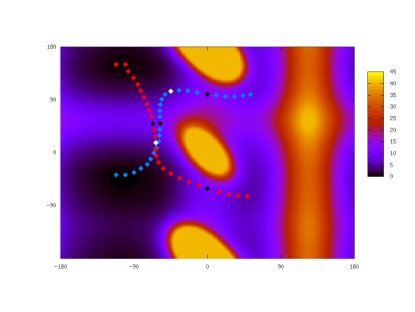
These simulations were performed at temperature $T=300K$, and assuming a diffusion coefficient $D=0.02$Ųps^-1 for all atoms. To determine the DFP we have performed 500 cycles of simulated annealing of the discretized Hamilton-Jacobi functional DFP , followed by a refinement stage where Conjugate Gradients were used. The effective energy $E_{eff}$ was estimated running a few ps of MD simulation starting from the minimum-energy conformation.

We will now show how the DFP analysis can provide valuable information about the dynamics of the transition, and about the determination of the transition state along the path. While other methods with similar purposes, e.g.SimAdv3 ; Ala3 , only provide a meta-dynamics, the DFP analysis yields information on the real-time evolution of the system. Even though time is no longer an independent variable of the calculation in the HJ formulation, the total time required to perform the transition from a conformation $x_{i}$ to a conformation $x_{f}$ can be computed as

$$t_{f}-t_{i}=\int_{x_{i}}^{x_{f}}dl\frac{1}{\sqrt{4D\left(E_{eff}+V_{eff}[x(l)]\right)}}$$ (26)

and the time spent in the neighborhood of each intermediate conformation (residence time along the path) is easily derived from the differential form of Eq. 26. The computed times for the C7ax$\to$C7eq and $\alpha_{L}\to\alpha_{R}$ transitions are 12.0 and 11.4 ps, respectively. Notice, that this is the most probable transition time, and not the mean first passage, or Kramers time carolifunct .

An analysis of the residence time along the path shows that in each of the two DFP’s, there are two points where the conformation of alanine dipeptide has shortest residence time. These points, indicated in Fig. (1) with black symbols, are located in the proximity of the saddle-points of the free energy landscape, as one would expect.

On the other hand, within the present formalism it is also possible to rigorously define the transition state along the path in terms of commitment analysis bunsen ; pandeTS . Following Eq. (2), once the DFP has been determined, the conformation $x_{ts}$ is easily obtained by requiring that the probability in the saddle point approximation to diffuse back to the initial configuration $x_{i}$, $P(x_{i}|x_{ts})$ equates that of evolving toward the final native configuration $x_{f}$, $P(x_{f}|x_{ts})$. In the saddle-point approximation, this condition leads to the simple equation:

$$\frac{U(x_{f})-U(x_{i})}{2k_{B}T}=S_{HJ}([x];x_{ts},x_{i})-S_{HJ}([x];x_{ts},x_{f}).$$ (27)

We want to point out that this definition of $x_{ts}$ neither relies on the use of any specific reaction coordinate, nor on the a priori knowledge of the free energy landscape, but is purely based on the properties of the diffusive dynamics followed by the system. Transition states computed using this prescription are shown in Fig.1 as white points. These results provide a clean example of the fact that the definition of transition-state in terms of commitment analysis can be used to locate the configuration of highest free-energy barrier only in the case of two-state transitions.

In conclusion, in the present work we have developed a new theoretical description of the protein folding reaction, based on Langevin dynamics. This approach allows for a huge reduction of the computational cost needed for obtaining information on the full reaction pathway. Within this framework, all-atom simulations for a dipeptide can be performed in just a few minutes on a regular desktop, to be compared with times of the order of a week required by standard MD to exctract the same amount of information. Moreover, we have shown that this theoretical tool provides important new insight into the protein folding problem. In fact, it allows to define, characterize and study the native and transition states and to determine the transition time at different temperatures. We have also exhibited, within this framework, a clear connection between the stability of the folded conformation and its small conformational entropy.

Applications of this formalism to the study of the conformational transitions of small proteins with all-atom models and implicit solvent are in progress.