Dynamical robustness of biological networks with hierarchical distribution of time scales

Abstract.

We propose the concepts of distributed robustness and $r$-robustness, well adapted to functional genetics. Then we discuss the robustness of the relaxation time using a chemical reaction description of genetic and signalling networks. First, we obtain the following result for linear networks: for large multiscale systems with hierarchical distribution of time scales the variance of the inverse relaxation time (as well as the variance of the stationary rate) is much lower than the variance of the separate constants. Moreover, it can tend to $0$ faster than $1/n$, where $n$ is the number of reactions. We argue that similar phenomena are valid in the nonlinear case as well. As a numerical illustration we use a model of signalling network that can be applied to important transcription factors such as NF$\kappa$B.

Keywords: Complex network; Relaxation time; Robustness; Signalling network; Chemical kinetics; Limitation; Measure concentration

1. Introduction

Robustness, defined as stability against external perturbations and internal variability, represents a common feature of living systems. The fittest organisms are those organisms that resist to diseases, to imperfections or damages of regulatory mechanisms, and that can function reliably in various conditions. There are many theories that describe, quantify and explain robustness. Waddington’s canalization, rigorously formalized by Thom describes robustness like structural stability of attractors under perturbations [Tho72, Wad57]. Many useful ideas on robustness have been imported from the theory of control of dynamical systems and of automata [Fat04, CAS05]. The new field of systems biology places robustness in a central position among the living systems organizing principles, identifying redundancy, modularity, and negative feed-back as sources of robustness [MWB⁺02, KOK⁺04, Kit04].

In this paper, we provide some justification to a different, less understood source of robustness.

Early insights into this problem can be found in the von Neumann’s [vN63] discussion of robust coupling schemes of automata. von Neumann noticed the intrinsic relation between randomness and robustness. Quoting him “without randomness, situations may arise where errors tend to be amplified instead of cancelled out; for example it is possible, that the machine remembers its mistakes, and thereafter perpetuates them”. To cope with this, von Neumann introduces multiplexing and random perturbations in the design of robust automata.

Related to this is Wagner’s [Wag05b, Wag05a] concept of distributed robustness which “emerges from the distributed nature of many biological systems, where many (and different) parts contribute to system functions”. To a certain extent, distributed robustness and control are antithetical. In a robust system, any localized perturbation should have only small effects. Robust properties should not depend on only one, but on many components and parameters of the system. A weaker version of distributed robustness is the $r$-robustness, when $r$ or less changes have small effect on the functioning of the system [DMKR06].

Molecular biology offers numerous examples of distributed robustness and of $r$-robustness. Single knock-outs of developmental genes in the fruit fly have localized effects and do not lead to instabilities [HWL02]. Complex diseases are the result of deregulation of many genetic pathways [WF06]. Transcriptional control of metazoa is based on promoter and enhancer regulating DNA regions that collect influences from many proteins [PG02]. Networks of regulating micro-RNA could be key players in canalizing genetic development programs [HS06]. Interestingly, computer models of gene regulation networks [vDMMO00] have distributed robustness with respect to variations of their parameters. Flux balance analysis in-silico studies of the effects of multiple knock-outs in yeast S.cerevisiae identified sets of up to eight interacting genes and showed that yeast metabolism is less robust to multiple attacks than to single attacks [DMKR06].

Let us formulate the problem mathematically. A property $M$ of the biological system is a function of several parameters of the system, $M=f(K_{1},K_{2},\ldots,K_{n})$. Let us suppose that the parameters $(K_{1},K_{2},\ldots,K_{n})$ are independent random variables. There are various causes of variability: mutations, across individuals variability, changes of the functional context, etc. For definitions of robustness we can start from inequality: $Var(M)\ll Var(K_{i}),\,1\leq i\leq n$.

In order to avoid the problem of units and supposing that $M,K_{i}>0$, we can use logarithmic scale:

Definition 1: $M$ is robust with respect to distributed variations if the variance of $M$ is much smaller than the variance of any of the parameters:

(1) $$Var(\log M)\ll Var(\log K_{i}),\,1\leq i\leq n.$$

We can also say that say that $M$ “concentrates” on its central value $M_{c}$.

Let us consider $r$-index subsets $I_{r}=\{i_{1},i_{2},\ldots,i_{r}\}\subset\{1,2,\ldots,n\}$ for given $r$. Let $K_{i}^{0},i=1,\ldots,n$ be the central values of the parameters. For given $I_{r}$, the perturbed values $K_{i}$ are obtained by multiplying $r$ selected central values by independent random scales $s_{i}>0,i=1,\ldots,r$, $K_{i}=K_{i}^{0}s_{i},i\in I_{r}$.

Definition 2: $M$ is robust with respect to $r$ variations or $r$-robust if for any $I_{r}$:

(2) $$Var(\log M)\ll Var(\log s_{i}),\,i\in I_{r}.$$

$r$-robustness holds if (2) is valid for any deterministic choice of $r$ targets. If the target set $I_{r}$ is randomly chosen we shall speak of weak $r$-robustness. We call robustness index the maximal value of $r$ such that the system is $r-$robust.

The above definitions are inspired from biological ideas. Our first definition corresponds to Wagner’s distributed robustness [Wag05a]. It expresses the fact that $M$ is not sensitive to random variations of the parameters. $r$-robustness has been defined in [DMKR06] as resistance with respect to multiple mutations. $r$-robustness can also be interpreted as functional redundance meaning that the property $M$ is collectively controlled by more than $r$ parameters, and can not be considerably influenced by changing a number of parameters less than or equal to $r$. One should also notice the introduction of a new concept. Even if there are $r$ critical targets (for instance genes whose mutations lead to large effects) the probability of hitting these $r$ targets randomly, could be small. We have introduced the weak $r$-robustness to describe this situation.

Robustness with respect to distributed variations defined by can be a consequence of the Gromov-Talagrand concentration of measure in high dimensional metric-measure spaces [M.95, Gro99]. In Gromov’s theory the concentration has a geometrical significance: objects in very high dimension look very small when they are observed via the values of real functions (1-Lipschitzian). This represents an important generalization of the law of large numbers and has many applications in mathematics.

In this paper we choose a signaling module example as an illustration of the concept of distributed robustness. The robust property that we study here is the relaxation time of a biological molecular system modeled as a network of chemical reactions. Relaxation time is an important issue in chemical kinetics, but there exists biological specifics. A biological system is a hierarchically structured open system. Any biological model is necessarily a submodel of a bigger one. After a change of the external conditions, a cascade of relaxations takes place and the spatial extension of a minimal model describing this cascade depends on time. Timescales are important in signalling between cells and between different parts of an organism. It is therefore important to know how the relaxation time depends on the size and the topology of a network and how robust is this time against variations of the kinetic constants.

The structure of this paper is the following. First, we extend the classical results on limiting steps of stationary states of one-route cyclic linear networks onto dynamic of relaxation of any linear network. This allows us to relate the relaxation time of a linear network with hierarchical distribution of time scales to low order statistics of the network constants and to prove the distributed robustness of this relaxation time. Last, using a model of the NF$\kappa$B signaling module as an example, we show that similar results apply to nonlinear networks. For this nonlinear network, the robustness of another characteristic time, the period of its oscillations is studied as well.

2. Limitation of relaxation in linear reaction networks

First we consider a linear network of chemical reactions. In a linear network, all the reactions are of the type $A_{i}\rightarrow A_{j}$ and the reaction rates are proportional to the reagents $A_{i}$ concentration.

The dynamics of the network is described by:

(3) $$\dot{c}=Kc$$

where $K$ is the matrix of kinetical parameters.

We call a linear network weakly ergodic , if for any initial state $c(0)$ there exists a limit state $\lim_{t\rightarrow\infty}\exp(Kt)\,c(0)$ and the set of all these limit states for all initial conditions is a one-dimensional subspace (for all $c$, $\lim_{t\rightarrow\infty}\exp(Kt)\,c=\lambda(c)c^{*}$, $\lambda(c)\in{\mathbb{R}}$.

The ergodicity of the network follows from its topological properties.

A non-empty set $V$ of graph vertexes forms a sink, if there are no oriented edges from $A_{i}\in V$ to any $A_{j}\notin V$. For example, in the reaction graph $A_{1}\leftarrow A_{2}\rightarrow A_{3}$ the one-vertex sets $\{A_{1}\}$ and $\{A_{3}\}$ are sinks. A sink is minimal if it does not contain a strictly smaller sink. In the previous example, $\{A_{1}\}$, $\{A_{3}\}$ are minimal sinks. Minimal sinks are also called ergodic components.

A linear conservation law is a linear function defined on the concentrations $b(c)=\sum_{i=1}^{n}b_{i}c_{i}$, whose value is preserved by the dynamics (3). The set of all the conservation laws forms the left kernel of the matrix $K$.

From ergodic Markov chain theory it follows that the following properties are equivalent:

i) the network is weakly ergodic.

ii) for each two vertices $A_{i},\>A_{j}\>(i\neq j)$ we can find such a vertex $A_{k}$ that oriented paths exist from $A_{i}$ to $A_{k}$ and from $A_{j}$ to $A_{k}$. One of these paths can be degenerated: it might be $i=k$ or $j=k$.

iii) the network has only one minimal sink (one ergodic component).

iv) there is an unique linear conservation law, namely $b(c)=\sum_{i=1}^{n}c_{i}$.

Hence, the maximal number of independent linear conservation laws is equal to the maximal number of disjoint ergodic components.

Now, let us suppose that the kinetic parameters are well separated and let us sort them in decreasing order : $k_{(1)}\gg k_{(2)}\gg\ldots\gg k_{(n)}$. Let us also suppose that the network has only one ergodic component (when there are several ergodic components, each one has its longest relaxation time that can be found independently). We say that $k_{(r)},\,1\leq r\leq q$ is the ergodicity boundary if the network of reactions with parameters $k_{1},k_{2},\ldots,k_{r}$ is weakly ergodic, but the network with parameters $k_{1},k_{2},\ldots,k_{r-1}$ it is not. In other words, when eliminating reactions in decreasing order of their characteristic times, starting with the slowest one, the ergodicity boundary is the constant of the first reaction whose elimination breaks the ergodicity of the reaction graph.

Let $\lambda_{i}$ be the eigenvalues of the matrix $K$ (these satisfy $Re\lambda_{i}\leq 0$; furthermore if $Re\lambda_{i}=0$ then necessarily $\lambda_{i}=0$). Relaxation to equilibrium of the network is multi-exponential, but the longest relaxation time is given by :

(4) $$\tau=1/\min\{-Re\lambda_{i}|\lambda_{i}\neq 0\}$$

An estimate of the longest relaxation time can be obtained by applying the perturbation theory for linear operators to the degenerated case of the zero eigenvalue of the matrix $K$. We have $K=K_{<r}(k_{1},k_{2},\ldots,k_{r-1})+k_{r}Q$, where $K_{<r}$ is obtained from $K$ by letting $k_{r}=k_{r+1}=\ldots k_{n}=0$, $Q$ is a constant matrix up to terms that are negligible relative to $k_{r}$. From Lemma, the zero eigenvalue is twice degenerated in $K_{<r}$ and only once degenerated in $K$. One gets the following estimate:

(5) $$\overline{a}\frac{1}{k_{(r)}}\geq\tau\geq\underline{a}\frac{1}{k_{(r)}},$$

where $\overline{a},\underline{a}>0$ are some positive functions of $k_{1},k_{2},\ldots,k_{r-1}$ (and of the reaction graph topology).

Two simplest examples give us the structure of the perturbation theory terms for $\min_{\lambda\neq 0}\{-Re\lambda\}$.

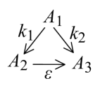
a) b)

Figure 1. Two basic examples of ergodicity boundary reaction: (a) Connection between ergodic components; (b) Connection from one ergodic component to element that is connected to the both ergodic components by oriented paths. In both cases, for $\varepsilon=0$, the ergodic components are $\{A_{2}\}$ and $\{A_{3}\}$.

1. Connection between ergodic components. For the reaction mechanism Fig. 1a $\min_{\lambda\neq 0}\{-Re\lambda\}=\varepsilon$, if $\varepsilon<k_{1}+k_{2}$.

2. Connection from one ergodic component to element that is connected to the both ergodic components by oriented paths. For the reaction mechanism Fig. 1b $\min_{\lambda\neq 0}\{-Re\lambda\}=\varepsilon k_{2}/(k_{1}+k_{2})+{\text{\em}o}\!\left(\varepsilon\right)$, if $\varepsilon<k_{1}+k_{2}$. For well separated parameters there exists a “trigger” alternative: if $k_{1}\ll k_{2}$ then $\min_{\lambda\neq 0}\{-Re\lambda\}\approx\varepsilon$; if, inverse, $k_{1}\gg k_{2}$ then $\min_{\lambda\neq 0}\{-Re\lambda\}={\text{\em}o}\!\left(\varepsilon\right)$.

More generally, let us suppose that the ergodicity boundary $k_{(r)}$ corresponds to a reaction that connects two disjoint ergodic components of the reaction graph $k_{(1)},\ldots,k_{(r-1)}$. Then we have:

(6) $$\tau=\frac{1}{k_{(r)}}+{\text{\em}o}\!\left(\frac{1}{k_{(r)}}\right)$$

If the ergodicity boundary $k_{(r)}$ corresponds to a reaction that connects one ergodic component to element that is connected to the both ergodic components by nonempty oriented paths (as in Fig. 1b), then we have the trigger alternative again, $1/\tau$ is either $k_{(r)}$, or ${\text{\em}o}\!\left(k_{(r)}\right)$.

Thus, the well known concept of stationary reaction rates limitation by “narrow places” or “limiting steps” (slowest reaction) should be complemented by the ergodicity boundary limitation of relaxation time. It should be stressed that the relaxation process is limited not by the classical limiting steps (narrow places), but by reactions that may be absolutely different. The simplest example of this kind is a catalytic cycle: the stationary rate is limited by the slowest reaction (the smallest constant), but the relaxation time is limited by the reaction constant with the second lowest value (in order to break the ergodicity of a cycle two reactions must be eliminated).

3. Robustness of relaxation time in linear systems

In general, for large multiscale systems we observe concentration effects: the log-variance of the relaxation time is much lower than the log-variance of the separate constants. For linear networks, this follows from well known properties of the order statistics [Leh75]. For instance, if $k_{i}$ are independent, log-uniform random variables, we have $Var[\log(k_{(r)})]\sim 1/n^{2}$. Here we meet a “simplex–type” concentration ([Gro99], pp. 234–236) and the log-variance of the relaxation time can tend to $0$ faster than $1/n$, where $n$ is the number of reactions.

For log-uniform parameters, $k_{(r)}$ has a log-beta distribution $\log(k_{(r)})\sim Beta(r,n+1-r)$.

We can obtain design principles for robust networks. Suppose we have to construct a linear chemical reaction network. How to increase robustness of the largest relaxation times for this network? To be more realistic let us take into account two types of network perturbation:

1. random noise in constants;

2. elimination of a link or of a node in reaction network.

Long routes are more robust for the perturbations of the first kind. So, the first receipt is simple: let us create long cycles! But long cycles are destroyed by link or node elimination. So, the second receipt is also simple: let us create a system with many alternative routes!

Finally the resources are expensive, and we should create a network of minimal size.

Hence, we come to a new combinatorial problem. How to create a minimal network that satisfies the following restrictions

1. the length of each route is $>L$;

2. after destruction of $D_{\rm l}$ links and $D_{\rm n}$ nodes there remains at least one route in the network.

In order to obtain the minimal network that fulfills the above constraints, we should include bridges between cycles, but the density of these bridges should be sufficiently low in order not to affect significantly the length of the cycles.

Additional restrictions could be involved. For example, we can discuss not all the routes, but productive routes only (that produce something useful).

For acyclic networks, we obtain similar receipts: long chains should be combined with bridges. A compromise between the chain length and number of bridges is needed.

We can also mention the role of degradation reactions (reaction with no products). Concentration phenomena are more accentuated when the number of degradation processes with different relaxation times is larger. Thus, one can increase robustness by increasing the spread of the lifetimes of various species.

The detailed discussion of this problem will be published separately.

4. Robustness of characteristic times in nonlinear systems: an example

The model

Our example is one of the most documented transcriptional regulation systems in eukaryote organisms: the signalling module of NF$\kappa$B. The response of this factor to a signal has been modeled by several authors [Ha02, La04, Na04, Ia04].

The transcription factor NF$\kappa$B is a protein (actually a heterodimer made of two smaller molecules p50 and p65) that regulates the activity of more than one hundred genes and other transcription factors that are involved in the immune and stress response, apoptosis, etc. NF$\kappa$B is thus the principal mediator of the response to cellular agression and is activated by more than 150 different stimuli : bacteria, viral and bacterial products, mitogen agents, stress factors (radiations, ischemia, hypoxia, hepatic regeneration, drugs among which some anticancer drugs). NF$\kappa$B has complex regulation, including inhibitor degradation and production, translocation between nucleus and cytoplasm, negative and positive feed-back. Under normal conditions, NF$\kappa$B is trapped in the cytoplasm where it forms a molecular complex with its inhibitor I$\kappa$B. Under this form, NF$\kappa$B can not perform its regulatory function, the complex can not penetrate the nucleus. A signal, that can be modeled by a kinase (IKK) frees NF$\kappa$B by degrading its inhibitor. Free NF$\kappa$B enters the nucleus and regulates the transcription of many genes, among which the gene of its inhibitor I$\kappa$B and the gene of a protein $A20$ that inactivates the kinase.

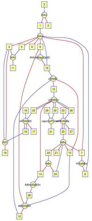
Figure 2. Model of NF$\kappa$B signalling. The non-linear reaction mechanism is represented as bipartite graph. The red edges indicate consumption, while the blue edges indicate production of molecules. There are $15$ chemical species and $31$ reactions.

Explaining context-dependent behavior of signal transduction pathways represents a great challenge in physiology. A rather popular explanation is pathway crosstalk. Another appealing explanation is that the signal could carry more information than it is expected due to its synchronous or asynchronous periodic nature [Na04]. These theories should be assessed experimentally and it is not our purpose to discuss their validity. Here we would like to study the robustness of the characteristic times of a non-linear molecular system. In particular, the double negative feed-back (via $I\kappa B$ and $A20$) is responsible for oscillations of NF$\kappa$B activity under persistent stimulation [Ha02, La04, Na04].

We use the model introduced in [La04] for the response of $NF\kappa B$ module to a signal. This model is represented in Fig. 2. The first reaction of the model is the activation of the kinase. In the absence of a signal the kinetic constant of the activation reaction is zero $k_{1}=0$, meaning that the kinase IKK remains inactive. The presence of a signal is modeled by a non-zero activation constant $k_{1}>0$, meaning that the kinase is activated.

We are interested in three characteristic times of the $NF\kappa B$ model: the period and the damping time of the oscillations and the largest relaxation time.

We have studied numerically the dependence of these time scales on the parameters of the model, which are the kinetic constants of the reactions. The damping time $\tau_{d}$ and the largest relaxation time $\tau_{max}$ were computed by linearizing the dynamical equations at steady state. The period of the oscillation has a rigorous meaning only for a limit cycle, when the oscillations are sustained. At a Hopf bifurcation and close to it, the inverted imaginary part of the conjugated eigenvalues crossing the imaginary axis provide good estimate for the period. Another method for computing the period is the direct determination of the timing between successive peaks. We have noticed that in logarithmic scale, the differences between the periods computed by the two methods were small, therefore we have decided to use the first method, which is more rapid. A criterion for the existence (observability) of the oscillations is the damping time to period ratio. This ratio is infinite for self-sustained oscillations, big for observable oscillations (when at least two peaks are visible). A low ratio means over-damped oscillations. We call the period an observable one, if the above ratio is larger than one.

$r$-robustness of the period

First, we have tested the $1$-robustness of the characteristic times. Each parameter has been multiplied by a variable, positive scale factor (changing from 0.001 to 1000), all the other parameters being kept fixed. The result can be seen in Fig. 3.

Large plateaus over which characteristic times are practically constant correspond to robustness. The period of the oscillations is particularly robust. For the damping time and the largest relaxation time we have domains of substantial variation. There are two types of such domains:

a) domains where $\frac{d\log(\tau)}{d\log(k)}\approx-1$.

b) domains where $|\frac{d\log(\tau)}{d\log(k)}|>1$.

where $k$ is the variable parameter.

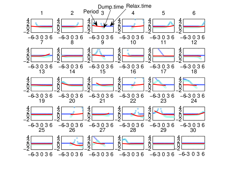
Figure 3. Log-log dependence of the characteristic times (blue crosses: largest relaxation time, cyan circles: dumping time, red line: period) on the scale factor that multiplies the value of one parameter, while all the other parameters are fixed. The scale factor varies from 0.001 to 1000 (from -6.9 to 6.9 in logarithm). Oscillations have limited existence regions (outside these regions they are overdamped; our subjective criterion for overdamping is a damping time over period ratio smaller than 1.75). There are also regions where oscillations are self-sustained. The limits of these regions are Hopf bifurcation points, where the damping time and the largest relaxation time diverge. Inside these regions, the damping time and the largest relaxation time are infinite and not represented.

The first type of behavior is the same as the one of linear networks. When changing only one parameter, there are domains in $k$ on which $k_{(r)}$ changes proportionally to $k$ (this corresponds to $k=k_{(r)}$). In other words, this happens when the perturbation acts on the ergodicity boundary. Outside these domains, $k_{(r)}$ is constant, which means a plateau in the graph.

The second type of behavior exists only for non-linear networks and is related to bifurcations. The variation of one parameter can bring the system close to a bifurcation (for the $NF\kappa B$ model, this is a Hopf bifurcation) where the relaxation time diverges.

The in silico experiment shows that the largest relaxation time is not $1$-robust; this time can be changed by modifying only one parameter. The damping time has similar behavior being even less robust (some plateaus of the largest relaxation time are higher than the damping time, which continues to decrease; consider for instance the effect of $k_{9}$ in Fig. 3).

As also noticed by the biologists [Na04], the period of the oscillations is $1$-robust. We do not have a rigorous explanation of this property. An heuristic explanation is the following. Close to the Hopf bifurcation two conjugated eigenvalues $\lambda\pm i\mu$ of the Jacobian cross the imaginary axis of the complex plane; $\lambda$ vanishes which explains the divergence of the relaxation time, while $\mu$, whose inverse is the period, does not change much. However, this is not a full explanation because it does not say what happens far from the Hopf bifurcation point.

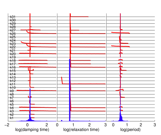
Figure 4. Parameter sensitivity study; distributions of the characteristic times when different parameters are, in turn, multiplied by a log-uniform (between 0.1 and 10), random scale factor, while all the other parameters are fixed. Distributions corresponding to various parameters are spread out vertically. The lower-most, bar-plotted distribution is the average of all the distributions and corresponds to choosing randomly the parameter to be modified. 1-robustness means that all distributions are concentrated (their spread in log-scale is small). Weak 1-robustness means that only the average distribution is concentrated.

Parameter sensitivity

Not all the parameters have the same influence on the characteristic times. This can already be seen in Fig. 3. In order to quantify these differences we have computed the distributions of the characteristic times when one parameter is multiplied by a log-uniform random scale, all the other parameters being fixed. This computation, whose results are represented in Fig. 4 is also a first step towards testing weak $r$-robustness.

Although rather robust, the period is not constant. Several parameters induce relatively significant changes of this quantity. In the order of increasing strength of their effect on the period, these parameters are : $k_{7},k_{9},k_{15},k_{23},k_{22},k_{26}$. Among these, $k_{22},k_{26},k_{9}$ expressing the transcription rates of mRNA-I$\kappa$B, the translation rates of I$\kappa$B, and the biding rate of the kinase to the NF$\kappa$B-I$\kappa$B complex are particularly interesting because by changing them, one can increase and also decrease the period. These results confirm and complete the findings of [Ia04]. The parameters that have the greatest influence on the period are the kinetic constants of the production module of I$\kappa$B : $k_{22},k_{26}$. We should emphasize the very different timescales of these reaction (one rapid $k_{22}=5\,\,10^{-1}$ and the other very slow $k_{26}=5\,\,10^{-7}$). The strong influence of NF$\kappa$B influx $k_{15}$ on the period, missed in [Ia04], is present here. Interestingly, the delay produced in the transcription/translation module of A20 have smaller effect on the period than the delay produced by the I$\kappa$B production module. Less obvious is the effect of $k_{7},k_{9}$ (binding of IKK to I$\kappa$B or to the complex) on the period, detected as important both here and in [Ia04].

The damping time to period ratio represents a criterion for observability of the oscillations. In order to increase the number of visible peaks, one should increase the above ratio. Because the period is robust, this is equivalent to increasing the damping time. Figs.3,4 show that this is possible in many ways by changing only one parameter (decrease of $k_{3}$, or $k_{9}$, or $k_{17}$, or $k_{18}$, or $k_{23}$, or $k_{27}$ or increase of $k_{4}$, or $k_{16}$, or $k_{20}$, or $k_{22}$, or $k_{26}$).

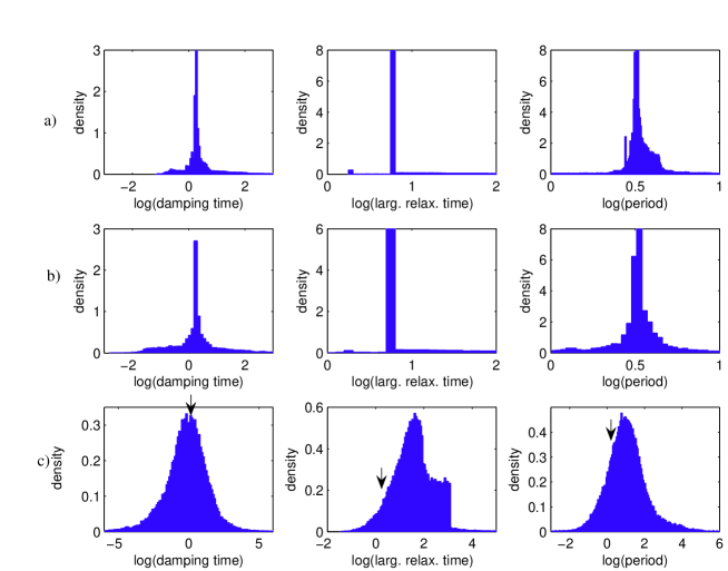
Figure 5. Distributions of characteristic times for log-uniform (between 0.1 and 10), independent random scales multiplying the kinetic parameters. We have changed a) one parameter, randomly chosen; b) two parameters, randomly chosen; c) all the parameters. The unperturbed values of the characteristic times are indicated with arrows. The concentration of the distributions at a) and b) shows that The period and the relaxation time are weakly 1- and 2-robust. The variation of all parameters produce long tailed distributions (that can be fitted by log-generalized logistic distributions) of the period and of the damping time, slightly biased relative to the unperturbed values (the bias of the period is positive, suggesting that it is easier to increase, than to decrease the period by random perturbations). The distribution of the relaxation time can be described as a mixture of a log-generalized logistic, and of a log-beta distribution. Let us remind that order statistics for log-uniform, independent variables follow log-beta distributions.

Weak $r$-robustness of all the characteristic times

The divergence of the relaxation time close to a bifurcation does not necessarily imply the absence of weak $r$-robustness or of distributed robustness. The set of bifurcation points forms a manifold in the space of parameters, of codimension equal to the codimension of the bifurcation; in general, this set has zero measure  . The probability of being by chance close to a bifurcation is generally small.

We have tested the weak $r$-robustness of the characteristic times, by using independent, log-uniform distributions of the parameters over 2 decades interval. All the three relaxation times are weakly $r$-robust when $r$ is small (see Fig. 4, Fig. 5a,b). Thus, although controlable (there are critical parameters), the system is somehow robust. Only an informed choice of the right targets has an effect, random choice of a small number of targets is inefficient.

We have also tested distributed robustness. Interestingly, when all the parameters take independent log-uniform values, the distributions of characteristic times, are much broader than the ones induced by changing a small number of parameters (see Fig. 5c). Neither the longest relaxation time, nor the damping time have distributed robustness. Nevertheless, the period is slightly more robust that the other characteristic times. In logarithmic scale, the distributions of the dumping time and of the period have exponential tails, with different decays rates towards $\infty$ and $-\infty$. These distributions (a possible fit is by generalized log-logistic distributions) have longer tails (in log scale) than log-normal distributions that are sometimes observed in biology [LDS⁺04, Kon04, BSRK05, FTK⁺05, LSA01]. The tails are also longer than the ones of the Tracy-Widom distribution characterizing largest eigenvalues of certain classes of random matrices [TW96, Sos02]. These long tails are related to the critical retardation phenomena [Gor04] close to the Hopf bifurcation (see also Fig. 3). The distribution of the relaxation time can be seen as a mixture between a log-normal and a log-generalized logistic distribution.

In order to quantify $r$-robustness we have plotted in Fig. 6 the dependence of the log variance of the characteristic times on $r$, the number of the perturbed parameters. For a property governed by simplex concentration (for instance the largest relaxation time of a linear network) one would expect the existence of a well defined robustness index. For $r$ values smaller than or equal to the robustness index, the system is $r$-robust, while for larger values it is not. This would imply a large increase of the log-variance with $r$ before the robustness index, and a much slower increase after. In Fig. 6 this is satisfied by the dumping time and by the largest relaxation time (robustness index between 1 and 7). The period has a completely different behavior, its log-variance being proportional to $r$. This means that no r-value is privileged, and in order to keep the period robust one should avoid multiple perturbations. This is more likely a cube concentration phenomenon, when the effect of different parameters is cumulative.

However, the log-variance of the period can not increase indefinitely. Even when perturbing all the parameters of the system, this log-variance remains about half smaller than the log-variance of the dumping time; it is even smaller if we consider only observable oscillations (big dumping time to period ratio). Concentration means that the slope of the linear dependence of the log-variance of the period on $r$ will tend to zero in an hierarchy of models of increasing complexity. The limit behavior can not be tested here because we analyze only one model, and not an hierarchy.

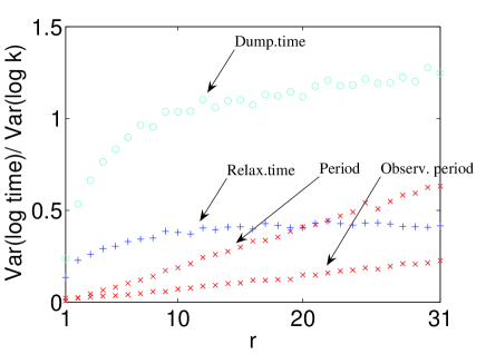
Figure 6. Log variance of the characteristic times as function of $r$, the number of perturbed parameters. The choice of the $r$ parameters is random (uniform) and the values of the random scales are independent, log-uniform (between 0.1 and 10). Some statistical samples correspond to overdamped oscillations ( dumping time / period ratio $<$ 1); these samples were rejected when computing the log-variance of the observable period.

5. Discussion and conclusions

We demonstrated the possibility of a new kind of robustness of biological systems. This type of robustness has geometrical origin, being related to the high dimension in which variability sources act. There are two basic types of such geometrical effects: cube type of concentration, or simplex type.

The classical example of the cube concentration gives the central limit theorem, when the robust property is the sum of many ($n$), independent contributions. For concentration of this type, the relative standard deviation decreases as $1/\sqrt{n}$. The classical example of the simplex concentration, is the situation when the robust property depends on the $k$-st in order effect (parameter) in a collection of of many ($n$) effects (parameters), for example, on the smallest, the largest or the second one. For concentration of this type, the relative standard deviation decreases much faster, as $1/n$. We have provided strong arguments that the robustness of the largest relaxation time in large multiscale networks with hierarchically distributed timescales is of the simplex type. The concentration of the period of a nonlinear oscillator seems to be of the cube type. This is coherent with the fact that the period results from the cumulative effect of various delay sources.

We have also defined the concepts of distributed robustness and $r$-robustness that occur naturally in cell physiology and molecular biology. The robustness index is the maximal integer $r$ such that the system is $r$-robust. For analysis of networks we discussed two types of noise: random noise in constants and destruction of links. The necessity of robustness to both types leads to a new combinatorial problem: How to create a minimal network that has sufficiently long routes (the length of each route is $>L$), and, at the same time, sufficiently many routes: after destruction of $D_{\rm l}$ links and $D_{\rm n}$ nodes there remains at least one route in the network.

In a recent work Rand [RSSM06] introduces the flexibility dimension that quantifies the range of evolution of clocks. This notion applies to multitask evolution, simultaneously fulfilling several objectives. By using linear response theory the authors proposed a method to compute the directions in the characteristic space that are not robust to changes of the parameters: the flexibility dimension is the largest linear space of characteristics that contains non-robust directions. Our notion of robustness index is different because it does not follow from linear response and more importantly it applies to parameters and not to characteristics (it is the maximum number of parameters that can be changed without sensible effect on the characteristics). Nevertheless it seems that the flexibility dimension and the robustness index have properties in common: they are both small for simple networks and they tend to be increased by the loop complexity and by the unevenness of the lifetimes of various species.

Concerning the analyzed example, several conclusions are important. NF$\kappa$B dynamics belongs to the category of ultradian oscillators. As for circadian oscillators [RSSM06], the period of the oscillations is a relatively robust property. Even if the biological role of these oscillations has not yet been proven (for some conjectures the reader can refer to [Na04]), it is important to known that the robustness applies to different timescales. A specificity of the the NF$\kappa$B system is the proximity to a bifurcation. Two non-linear phenomena could be relevant for the behavior of the signalling system : the critical retardation and the excitability. The first property would produce long tail distributions of the damping time of the oscillations and interesting possibilities for synchronization. The second property could raise the efficiency of the regulatory role of NF$\kappa$B by increasing the amplitude of its response to signals.

The robustness of a system is related to its complexity. More precisely, it is given by two levels of complexity: the one on which the sources of variability act and the one of its dynamics. The higher is the level of complexity where the variability acts and the lower is the level of dynamical complexity, the higher is the robustness. In order to test the concentration from high dimension rigorously one needs to build an hierarchy of models obtained one from another by model reduction. Parameters of simpler models in the hierarchy are functions of packages of parameters (“atoms”) of more complex models. Independent perturbations of the atoms produce less variability than overall perturbation of packages. These ideas will be presented in detail in a future work.

References

- [BSRK05] M. Begtson, A. Stahlberg, Patrik Rorsman, and Mikael Kubista. Gene expression profiling in single cells from the pancreatic islets of langerhans reveals lognormal distribution of mrna levels. Genome Research, 15:1388–1392, 2005.
- [CAS05] J.M. Chaves, R. Albert, and E.D. Sontag. Robustness and fragility of boolean models for genetic regulatory networks. J. Theoretical Biology, 235:431–449, 2005.
- [DMKR06] D. Deustcher, I. Meilijson, M. Kupiec, and E. Ruppin. Multiple knockout analysis of genetic robustness in the yeast metabolic network. Nature Genetics, 9:993–998, 2006.
- [Dri79] H. Driesch. The Science and Philosophy of the Organism. AMS, New York, 1979. originally published by Adam and Charles Black, London, 1908.
- [Fat04] N. Fates. Robustesse de la dynamique des syst mes discrets : le cas de l’asynchronisme dans les automates cellulaires. Phd, ENS Lyon, 2004.
- [FTK+05] C. Furusawa, T.Suzuki, A. Kashiwagi, T. Yomo, and K. Kaneko. Ubiquity of log-normal distributions in intra-cellular reaction dynamics. Biophysics, 1:25–31, 2005.
- [Gor04] A.N. Gorban. Singularities of transition processes in dynamical systems. Electronic Journal of Differential Equations, Monograph 05, 2004.
- [Gri04] G. Grinstein. Can complex structures be generically stable in a noisy world? IBM J. Res. Dev., 48:5–12, 2004.
- [Gro99] M. Gromov. Metric structures for Riemannian and non-Riemannian spaces, Progr.Math. 152. Birkhauser, Boston, 1999.
- [Ha02] A. Hoffmann and al. The ib-nf-b signaling module: temporal control and selective gene activation. Science, 298:1241–1245, 2002.
- [HS06] E. Hornstein and N. Shomron. Canalization of development by micrornas. Nature Genetics, 38:S20–24, 2006.
- [HWL02] B. Houchmanzadeh, E. Wieschaus, and S. Leibler. Establishment of developmenal precision and proportions in the early drosophila embryo. Nature, 415:798–802, 2002.
- [Ia04] A.E.C. Ihekwaba and al. Sensitivity analysis of parameters controlling oscillatory signalling in the nf-b pathway: the roles of ikk and ib. Syst.Biol., 1:93–102, 2004.
- [Kit04] H. Kitano. Biological robustness. Nature Reviews, 5:826–837, 2004.
- [KOK+04] H. Kitano, K. Oda, T. Kimura, Y. Matsuoka, M. Csete, J. Doyle, and M. Muramatsu. Metabolic syndrome and robustness tradeoffs. Diabetes, 53:S6–S15, 2004.
- [Kon04] T. Konishi. Three-parameter lognormal distribution ubiquitously found in cdna microarray data and its application to parametric data treatement. BMC Bioinformatics, 5, 2004.
- [La04] T. Lipniacki and al. Mathematical model of nf-b regulatory module. J.Theor.Biol., 228:195–215, 2004.
- [LDS+04] D. Liu, D.M.Umbach, S.D.Pedada, L. Li, P.W. Crockett, and C.R. Weinberg. A random-periods model for expression of cell-cycle genes. PNAS, 101:7240–7245, 2004.
- [Leh75] E.L. Lehmann. Nonparametrics. Holden-Day, San Francisco, 1975.
- [LSA01] E. Limpert, W.A. Stahel, and M. Abbt. Log-normal distributions across the sciences: keys and clues. BioScience, 51:341–352, 2001.
- [M.95] Talagrand M. Concentration of measure and isoperimetric inequalities in product spaces. Inst. Hautes Etudes Sci. Publ. Math., 81:73–205, 1995.
- [MWB+02] M. Morohashi, A. Winn, M.T. Borisuk, H. Bolouri, J. Doyle, and H. Kitano. Robustness as a measure of plausability in models of biochemical networks. J.theor.Biol., 216:19–30, 2002.
- [Na04] D.E. Nelson and al. Oscillations in nf-b signaling control the dynamics of gene expression. Science, 306:704–708, 2004.
- [PG02] M. Ptashne and A. Gann. Genes and Signals. CSHL Press, Cold Spring Harbor, 2002.
- [RSSM06] D.A. Rand, B.V. Shulgin, J.D. Salazar, and A.J. Millar. Uncovering the design principles of circadian clocks: Mathematical analysis of flexibility and evolutionary goals. J. Theor. Biol., 238:616–635, 2006.
- [Sos02] A. Soshnikov. A note on universality of the distribution of the largest eigenvalues. J. Stat. Phys., 108:1033–1056, 2002.
- [Tho72] R. Thom. Structural stability and morphogenesis: an outline of a general theory of models. W.A. Benjamin, New York, 1972.
- [TW96] C.A. Tracy and H. Widom. On orthogonal and symplectic matrix ensembles. Comm. Math. Phys., 177:727–754, 1996.
- [vDMMO00] G. von Dassow, E. Meir, E. M. Munro, and G. M. Odell. The segment polarity network is a robust developmental module. Nature, 406:188–192, 2000.
- [vN63] J. von Neumann. Probabilistic logics and the synthesis of reliable organisms from unreliable components. In J. von Neumann Collected works vol.5, Oxford, 1963. Pergamon Press.
- [Wad57] C.H. Waddington. The strategy of genes. Allen and Unwin, London, 1957.
- [Wag05a] A. Wagner. Distributed robustness versus redundancy as causes of mutational robustness. BioEssays, 27:176–188, 2005.
- [Wag05b] A. Wagner. Robustness and evolvability in living systems. Princeton University Press, Princeton, Oxford, 2005.
- [WF06] H. Watkins and M. Farrall. Genetic susceptibility to coronary artery disease: from promise to progress. Nature Reviews Genetics, 7:163–173, 2006.