Adaptive Filtering Enhances Information Transmission in Visual Cortex

Abstract

Sensory neuroscience seeks to understand how the brain encodes natural environments. However, neural coding has largely been studied using simplified stimuli. In order to assess whether the brain’s coding strategy depend on the stimulus ensemble, we apply a new information-theoretic method that allows unbiased calculation of neural filters (receptive fields) from responses to natural scenes or other complex signals with strong multipoint correlations. In the cat primary visual cortex we compare responses to natural inputs with those to noise inputs matched for luminance and contrast. We find that neural filters adaptively change with the input ensemble so as to increase the information carried by the neural response about the filtered stimulus. Adaptation affects the spatial frequency composition of the filter, enhancing sensitivity to under-represented frequencies in agreement with optimal encoding arguments. Adaptation occurs over 40 s to many minutes, longer than most previously reported forms of adaptation.

The neural circuits in the brain that underlie our behavior are well suited for processing of real-world – or natural – stimuli. These neural circuits, especially at the higher stages of neural processing, may be largely or completely unresponsive to many artificial stimulus sets used to analyze the early stages of sensory processing and, more generally, for systems analysis. Thus, natural stimuli may be necessary to study higher-level neurons. Characterizing neural responses to natural stimuli at early or intermediate stages of neural processing, such as the primary visual cortex, is a necessary step for systematic studies of higher-level neurons. Neural responses are also known to be highly nonlinearTheunissen et al. (2000); Sceniak et al. (2002); Nolt et al. (2004) and adaptiveMaffei et al. (1973); Shapley and Victor (1979); Shapley and Enroth-Cugell (1984); Ohzawa et al. (1985); Saul and Cynader (1989); Smirnakis et al. (1997); Brenner et al. (2000a); Dragoi et al. (2000); Fairhall et al. (2001); Chander and Chichilnisky (2001); Baccus and Meister (2002); Kohn and Movshon (2004); Solomon et al. (2004); Victor (1987); Brown and Masland (2001); Movshon and Lennie (1979); Albrecht et al. (1984), making them difficult to predict across different stimulus setsDavid et al. (2004). Therefore, even early in visual processing, characterizations based on simplified stimuli may not be adequate to understand responses to the natural environment.

For these reasons there has been a great deal of interest in studying neural responses to complex, natural stimuli (for example, see refs Theunissen et al. (2000); David et al. (2004); Baddeley et al. (1997); Theunissen et al. (2001); Ringach et al. (2002); Smyth et al. (2003); Felsen et al. (2005)). However, the relationship between coding of natural and laboratory stimuli remains elusive due to the difficulty of characterizing neurons – assessing their receptive fields – from responses to natural stimuli, as we now describe.

A simple and commonly-used model of neural responses is the linear-nonlinear modelde Boer and Kuyper (1968); Rieke et al. (1997). In this model, the response of the neuron depends on linear filtering of the stimulus luminance values S by a receptive field L defined over some region of space and time. Mathematically, the filter output at time $t$ is a sum over the spatial positions ($x$,$y$) and temporal delays $t^{\prime}$ to which the neuron’s response is sensitive: $\sum_{x,y,t^{\prime}}$L$(x,y,t-t^{\prime})$S$(x,y,t^{\prime})$, which we abbreviate as L*S. The output of this filter is then passed through a nonlinear function $f$ to yield the neuron’s response $r$: $r(t)=f($L*S$)$. The nonlinearity incorporates the fact that the firing rate cannot be negative and other aspects of neural response such as threshold, saturation, and sensitivity or insensitivity to changes in stimulus polarity. We will use the terms neural filter or receptive field throughout this paper to mean the linear part L of the linear-nonlinear model.

Traditionally, neural receptive fields have been estimated as the spike-triggered average stimulus (STA; with appropriate correction for autocorrelation of the inputs)Theunissen et al. (2000, 2001); Ringach et al. (2002); Smyth et al. (2003); de Boer and Kuyper (1968); Rieke et al. (1997) or by related methodsBrenner et al. (2000a); Felsen et al. (2005); Rust et al. (2005). These methods give unbiased results for linear systems for any stimulus ensemble or for nonlinear systems if the ensemble is Gaussian random noise. However, they produce systematic deviations from the true filter of nonlinear “linear-nonlinear” neurons probed with natural stimuli (or other non-Gaussian stimuli), even in situations where the only nonlinearity is due to a conversion of the output of a linear receptive field to firing rateRingach et al. (2002); Sharpee et al. (2004). This happens because natural stimuli, unlike Gaussian stimuli which may be completely described by pairwise correlations, have strong higher-order as well as pairwise correlationsRuderman and Bialek (1994); Field (1994); Simoncelli and Olshausen (2001). The higher-order correlations may be viewed as what distinguishes natural from random Gaussian stimuli. The bias in the filter estimate calculated using the Gaussian or linear assumption increases with the strength of the nonlinearity and with the strength of stimulus correlations beyond second orderRingach et al. (2002); Sharpee et al. (2004), not vanishing even with infinite data.

Recently an information-theoretic method has been developed that correctly estimates receptive fields of nonlinear model neurons (with extensions to multiple linear filters) for arbitrary stimulus ensembles regardless of the strength of multi-point correlations, even in cases where the STA is zeroSharpee et al. (2004). According to this method, one searches for the spatiotemporal filter L whose output, L*S, carries the most mutual information with the experimentally measured neuronal response $r(t)$. In practice, this is done via a gradient ascent procedure, searching in the space of all possible spatiotemporal receptive fields or filters to find the most informative one (referred to as “the most informative dimension”, or MID). We can then calculate the nonlinearity associated with the MID from the data as the probability of a spike given the filter output; there is no need to make any assumption about the shape of the nonlinearity.

Similarly to other “spike-triggered” methods, the MID method compares two probability distributions of outputs for a given filter: the distribution of outputs that occur before (or trigger) a spike, and the distribution of outputs over the entire stimulus ensemble regardless of neural response. If a filter represents a stimulus feature that affects neural responses, then certain values of its output will be more probable before a spike, and so the two distributions should differ from one another. The various methods all seek filters that maximize the difference between the two distributions, but differ in the measure of this difference. For the STA, the measure is the change in the mean of the two distributions; for the spike-triggered covariance methodBrenner et al. (2000a); Felsen et al. (2005); Rust et al. (2005), it is the change in the variance; and for the MID, it is an information-theoretic measure (the Kullback-Leibler distance) that corresponds to the mutual information between the filter output and the spikes. The information-theoretic measure is more general than the mean or variance, because it is sensitive to correlations of all orders, which in part explains the success of the MID method in estimating neural filters from responses to natural stimuli. Here we apply this method for the first time to neural data, focusing on the single-filter model, to address the question of whether and how V1 receptive fields adapt to natural stimuli.

I Receptive fields from noise vs. natural scenes

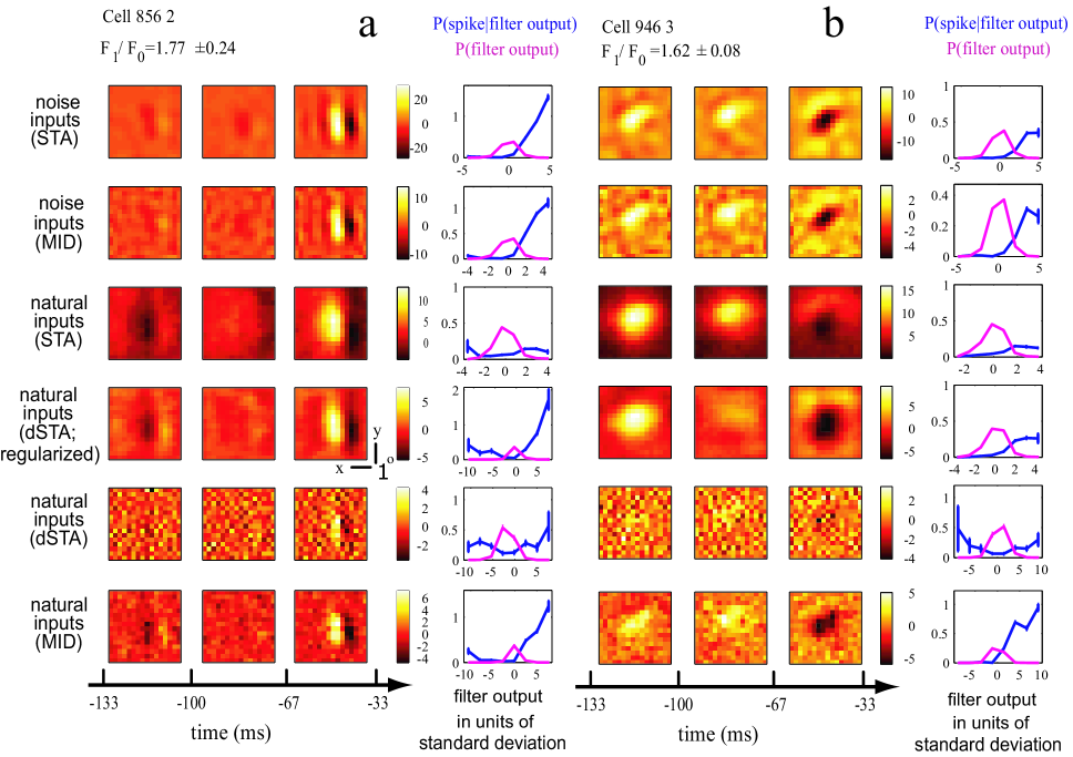
Figure 1: Filters and nonlinearities for two simple cells. Top to bottom: STA and MID for noise ensemble; STA, dSTA, dSTA with regularization, and MID for natural ensemble. Spatiotemporal receptive fields have three time frames covering the indicated interval (-133 to -33 ms). In the right-most column for each filter we plot the probability distribution of filter outputs in the stimulus ensemble (magenta) and the spike probability given the filter output (blue; values of the $y$ axis refer to these probabilities). The color scale shows the filter in units of its average noise level (see Supplementary Methods). $x$-$y$ scale bars: 1^o. Error bars show standard errors of the mean in all figures.

We studied 40 simple cells (as characterized by responses to optimal moving gratingsSkottun et al. (1991)) in anesthetized cat V1 (complex cells can also be characterized by the MID methodSharpee et al. (2004) and will be considered in a future publication). We probed these neurons with natural and white noise inputs. These inputs differ in two important respects. First, they have very different pairwise correlations, which are described by the power spectra. The power spectrum of a white noise ensemble does not depend on either spatial or temporal frequency within a certain range, while the power spectrum of natural inputs depends on spatial frequency $k$ as $\sim 1/k^{2}$ under a wide variety of conditionsRuderman and Bialek (1994); Simoncelli and Olshausen (2001); Field (1987); Dong and Atick (1995) (spatiotemporal statistics have similar structureDong and Atick (1995)). Second, natural scenes have strong statistical correlations beyond second order that cannot be described by the power spectrum, as evident for example in the much greater incidence of oriented edges in natural scenes than in Gaussian noise with the same power spectrumRuderman and Bialek (1994); Simoncelli and Olshausen (2001).

To estimate spatiotemporal receptive fields or neural filters from responses to noise and natural stimuli, we applied both the linear systems and information-theoretic methods. The resulting estimated filters and STAs for two example cells are shown in Fig. 1. With respect to responses to the noise ensemble, we found the filter for each cell either as the traditional STA or as the MIDSharpee et al. (2004). As expected for white noise stimuli, the two estimates do not differ significantly from each other for the illustrated cells or for most cells ($p>0.05$ for 31 out of 40 cells; $t$-test, see Supplementary Methods); the remaining differences can be attributed to the residual spatial correlations in the white noise ensemble (cf. Fig. 3b). This agreement illustrates the basic validity of the MID method under circumstances where the STA offers an independent unbiased estimate.

For responses to the natural stimulus ensemble, we calculated the STA and corrected it for second-order correlations present in the natural ensemble to obtain a decorrelated STA (dSTA). This would describe the neuron’s filter if the neuron were linear. Because this procedure of correcting for stimulus correlations tends to amplify noise, we also calculated the dSTA using regularization to prevent such amplification – such decorrelation with regularization has been used in most previous work estimating neural filters from responses to natural signalsTheunissen et al. (2000); David et al. (2004); Ringach et al. (2002); Smyth et al. (2003); Felsen et al. (2005). Finally, we estimated the filter from natural inputs as the MID. As can be seen in Fig. 1, the MID produces an estimate of the filter for natural scenes that is much closer to the white noise filter than either the dSTA or the regularized dSTA. Across cells, the dSTA shows a greater difference from the white noise filter than does the natural ensemble MID, as judged by smaller correlation coefficients with either the noise ensemble STA or noise ensemble MID (40/40 cells, $p<10^{-6}$). This demonstrates that some of the differences between the neural filters obtained from natural and noise stimulation in the linear model are due to biases in the estimation of the natural filter that can be removed once the linear-nonlinear model is considered and the MID is computed. In Fig. 1, we also plot the nonlinear functions that show spike probability as a function of filter output. They are similar in shape for the MIDs of the two ensembles, and this behavior seems to be typical across cells.

We used the MIDs to estimate both the noise and natural filters in what follows. We studied all simple cells with a non-zero filter to both natural and noise inputs.

Despite the similarity of the filters obtained under the two conditions, cf. Fig. 1, a jackknife analysis of the errors in estimating the neural filters shows that the differences between the filters derived from noise and natural signals are statistically significant ($p<0.01$) for all cells. To investigate the source of these differences and to make connections with classic studies on neural responses to moving periodic patterns (gratings) of certain orientations and spatial frequencies, we compute the spatiotemporal Fourier transform of the filter in the two spatial dimensions and time. The position of the maximum of the Fourier transform at the grating temporal frequency is our prediction for the optimal grating orientation and spatial frequency for a particular neuron. We did not detect any systematic shifts in optimal orientation and only a small shift in optimal spatial frequency as assayed from noise filters, natural signals filters and grating stimuli, in agreement with previous findings using the regularized dSTASmyth et al. (2003); Felsen et al. (2005), see Supplementary Discussion.

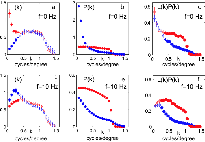
Figure 2: Neural filters compensate for changes in the input power spectrum. Average amplitude spectra of neural filters (a,d) and input ensembles (b,e) corresponding to natural (blue circles) and white noise (red circles) stimulation for temporal frequencies of 0 and 10 Hz. The spectra were taken along the optimal orientation for each cell by interpolating the discrete 2D Fourier transform. We use filled circles at frequencies where mean sensitivity was significantly different between the two ensembles (small circles for $p<0.05$ and large for $p<0.01$), and open symbols otherwise. (c, f) Plots of the product of the average neural filter and input ensemble amplitude spectra.

The most marked differences between the neural filters derived from natural vs. noise stimulation are seen by considering the entire shape of the spatial frequency tuning curves (Fig. 2 and Supplementary Figs 1 and 2) and not just the location of the single best spatial frequency. For each cell and temporal frequency, we calculated the spatial frequency profile along the cell’s preferred stimulus orientation using interpolation of the filter’s two-dimensional discrete Fourier transform. Note that our temporal resolution allowed analysis only at two temporal frequencies (0 Hz and 10 Hz, in each of two opposite directions of motion). Results at 10Hz did not depend on direction of motion so both directions were combined in Fig. 2, which shows the average tuning of the cells in our dataset. For low spatial frequencies sensitivity decreased (increased) to common (rare) inputs, while at middle and high spatial frequencies the sensitivity did not change. For example, at zero temporal frequency, low spatial frequencies are more common in the natural than in the white noise stimulus ensemble (Fig. 2b). Correspondingly, neurons became less sensitive to those frequencies during stimulation with natural inputs than during stimulation with noise inputs (Fig. 2a). In the case of non-zero temporal frequencies the trend is reversed, because the noise stimulus ensemble has more power at nearly all spatial frequencies than the natural stimulus ensemble (Fig. 2d, e). These changes in filter can be observed in the majority of cells, and are not simply due to adaptation in a small subset of cells. This is shown in Supplementary Fig. 1, which illustrates the spatial frequency sensitivities of the two example cells whose receptive fields are shown in Fig. 1, and Supplementary Fig. 2, which shows scatter-plots of spatial frequency sensitivity of noise vs. natural filters across all cells.

II Optimal filtering in a nonlinear system.

In retrospect, such shifts in spatial frequency sensitivity may be expected for neural coding to be optimal for both of two input ensembles (whit noise and natural stimuli) that have such vastly different power spectra as white noise and natural stimuliRuderman and Bialek (1994); Simoncelli and Olshausen (2001); Field (1987) (see Fig. 2b, e). In general it is difficult to map optimal coding strategy from one ensemble to another; however, it could be done if both of the stimulus ensembles were Gaussian so that they were entirely characterized by their power spectra. Suppose a neuron uses filter $L_{A}$ and nonlinearity $f_{A}$ to optimally encode Gaussian stimulus ensemble $A$ with spatiotemporal amplitude spectrum $P_{A}(k,\omega)$. What would then be an optimal strategy to encode Gaussian ensemble $B$ with amplitude spectrum $P_{B}(k,\omega)$? One solution is to leave the nonlinearity unchanged and to compensate for differences in the input power spectra by changing neural filter properties so that:

$$L_{A}(k,\omega)\cdot P_{A}(k,\omega)=L_{B}(k,\omega)\cdot P_{B}(k,\omega)$$ (1)

This will leave unchanged all statistics of neuronal response, and so in particular will leave invariant any statistical measures of optimality. Alternative strategies involving a change in nonlinearity cannot be optimal unless there are multiple optima, because if ensemble $A$ has a unique optimum, then the above strategy will give the unique optimum for ensemble $B$. (Note that, in response to an overall change in contrast, the nonlinearity can be rescaledBrenner et al. (2000a); Fairhall et al. (2001), but this is equivalent to a rescaling of the filter according to Eq. 1 with no change in nonlinearity.)

These conclusions about the receptive field and nonlinearity apply only to Gaussian stimuli. The higher-order correlations present in natural scenes may both lead to deviations from Eq. (1) in neural filters and cause changes in the shape of the nonlinearity. But in practice, the changes in the shape of the nonlinearity are small, and changes in neural filters that do take place act to compensate for changes in the input power spectrum as predicted from Eq. (1) (Fig. 2c,f). These changes in frequency sensitivity occur primarily at low spatial frequencies. No changes are observed at mid-to-high spatial frequencies, resulting in significant deviations from Eq. (1) in the middle range of frequencies. We can only speculate that other factors may limit the range of frequencies over which adaptation can occur.

III Adaptation Increases Information Transmission

The above optimal coding argument provides at least a qualitative explanation of observed receptive field changes. Most theories of optimal coding define optimality in information-theoretic terms. To test directly whether the information maximization argument applies to our data, we calculated the average mutual information between the filter output and the neural response; the response at a given time is simply taken as the presence or absence of a single spikeSharpee et al. (2004).

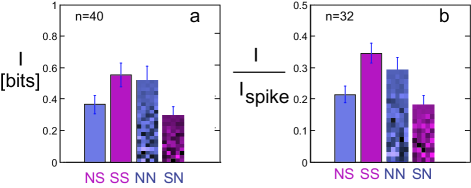
Figure 3: Receptive field adaptation increases information transmission. Bars show the mutual information between spikes and outputs of either noise (blue, N) or natural scenes (red, S) filter applied to natural scenes ensemble (solid) or noise ensemble (pixelated). NS, white noise filter applied to natural scenes ensemble; SS, natural scenes filter applied to natural scenes ensemble; NN, white noise filter applied to noise ensemble; SN, natural scenes filter applied to noise ensemble. The information values are given in bits (a) or in units of the total information carried by the arrival of a single spike $I_{spike}$Brenner et al. (2000b) (b).

The changes in receptive fields act to increase the information after changes in stimulus ensemble, and this information would be substantially reduced if receptive fields did not change with the ensemble. That is, the natural filter carries more information about responses to the natural ensemble than to the noise ensemble ($p<10^{-4}$, paired Wilcoxon two-tailed test), whereas the noise filter carries more information about responses to the noise ensemble than to the natural ensemble ($p=0.03$). The average information values across the population are shown in Fig. 3, and scatter-plots on a cell-by-cell basis are provided in Supplementary Fig. 4. Each filter produces roughly equal information about responses to its own ensemble: the difference in information values achieved by applying the noise filter to the noise ensemble versus applying the natural filter to the natural ensemble is not significant ($p=0.18$, paired Wilcoxon test). Each filter produces substantially less information about responses to the other ensemble ($p<10^{-4}$ for natural or noise ensemble filtered with natural versus noise filter; paired Wilcoxon tests), and there is no significant difference between the swapped combinations (natural filter applied to noise ensemble or visa versa, $p=0.06$, paired Wilcoxon test). We note that the changes in information are not due to overfitting or other computational artifacts, because information was calculated from responses to ensemble segments that were not used in calculating the filters, and the effects were not seen in data from a model linear-nonlinear cell with unchanging filter that was analyzed similarly, see Supplementary Information.

In addition to considering information $I$ in bits (Fig. 3a), we also measured information for each cell in units of $I_{\rm spike}$Brenner et al. (2000b), the information in the neuron’s response (as defined above) about the full stimulus (Fig. 3b). $I/I_{\rm spike}$ measures the fraction of the total possible information that is captured by the single most informative filter ($I_{\rm spike}$ is a separate measurement that was available only for a subset of cells, making the data set smaller). As can be seen, the MID captures roughly 35% of the possible information for simple cells. Each filter provides a greater fraction of the overall information when applied to its own ensemble than the other ($p\leq 10^{-4}$ for natural filter applied to natural vs. noise ensemble and for either ensemble filtered with natural vs. noise filter; $p=0.05$ for noise filter applied to natural vs. noise ensemble; paired Wilcoxon test).

IV Dynamics of receptive field adaptation

Even though the best linear-nonlinear model systematically changes with the stimulus ensemble, this does not establish that the neuron has changed its encoding strategy. The true encoding strategy may be complicated and nonlinear, so that even if it is static, the best linear-nonlinear estimate of it may change with the ensemble, much as the best linear approximation to a curve changes with position on the curve.

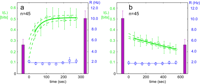
Figure 4: Adaptation dynamics. a,b, The neural filter derived from the last half of natural stimulation is applied to the first half of natural (a) or to the noise (b) ensemble. Symbols show information (green, left $y$ axis) and firing rate (blue, right $y$ axis) averaged across cells, versus time. The solid line is an exponential fit; dashed lines show one standard deviation based on the Jacobian of the fit [$p=0.01$ in a and $p=0.003$ in b using an $F$-test with null hypothesis of no time dependence]. The taller (shorter) red bars show information for the natural filter applied to natural (noise) inputs (as in Fig. 3, but $n=45$). The firing rates demonstrate that recordings are stable.

The most direct method to distinguish between an adaptive strategy and a complex but static coding strategy would be to estimate the filter as a function of time and see it change. This method yields very poor time resolution, because $\sim 5$ min of data are needed to estimate the filter, so adaptation that occurs on a faster timescale cannot be seen. Nonetheless we tried this method and saw appropriate, if weak, adaptation to noise stimuli even on this long time scale (see Supplementary Fig. 5). To achieve finer time resolution, we studied adaptation by measuring changes with time in the information carried by the output of a single, static filter; this information can be estimated from $\sim 30$ s of data. We used the following reasoning. If the coding is static, then the mutual information between this filter’s output and the neuron’s responses to a given ensemble should not systematically change in time. However, if the neuron’s receptive field adapts to the stimulus ensemble, then this information may systematically change in time. In particular, we take the static filter to be that characterizing a neuron when it is well adapted to a given ensemble – say the natural ensemble. When the neuron is newly exposed to a natural ensemble, the information carried by this filter should increase with increasing time of exposure to the natural ensemble, as the neuron adapts so that the filter that it actually uses to encode incoming stimuli into spikes becomes closer and closer to this static, fully adapted filter. Similarly, when the neuron is newly exposed to a noise ensemble, the information carried by this filter should decrease with increasing time of exposure to the noise ensemble, as the neuron’s own filter adapts to the noise and becomes less and less like the fully adapted natural scenes filter.

We derived filters from the last half of the 10-min presentations of each stimulus ensemble, when the neuron would be best adapted to the given ensemble if adaptation occurs. We then applied these static filters to both noise and natural stimuli, and measured information between spikes and filtered stimuli in successive 34-s periods during the first half of stimulus presentation (if the filter was derived from the second half of this stimulus) or in successive 68-sec periods during all of the presentation of the opposite ensemble. Most cells did not show significant adaptation when considered individually, presumably due to the variability in measuring information over such brief time periods. However, averaging over the entire population of simple cells revealed clear adaptation over time, consistent with an adaptive coding strategy (Fig. 4). The information progressively increased with time when natural inputs were filtered with the neural filter derived from the natural stimulus ensemble (Fig. 4a; see also Supplementary Discussion and Supplementary Fig. 6), while the information decreased with time when that same filter was applied to noise inputs (Fig. 4b).

Fits of a single exponential to the average data demonstrate that there is a statistically significant monotonic change with time, with time constants $\tau=42\pm 9$ s for adaptation to the natural ensemble and $\tau=22\pm 2$ min for adaptation to the noise ensemble. These time constants are consistent with the fact that we could not detect adaptation to the natural ensemble with the 5-min time scale of direct filter measurements, but we could detect adaptation to the noise ensemble (Supplementary Fig. 5). Note, however, that the time constants are based on the assumption of exponential decay, and do not exclude the possibility of multiple time scales, including scales faster than we were able to measure, or of alternative functional forms of decay.

We could not detect a significant trend with time in the information carried by the noise filter about either ensemble (see Supplementary Fig. 7). This is perhaps not surprising given that the average decrease in information for the noise filter applied to the noise versus natural ensembles was not significant ($p=0.14$, unpaired $t$-test), and that the slow time course of adaptation to the noise ensemble suggests that the filter we tested was not fully adapted to it (see also legend of Supplementary Fig. 7). Nonetheless, the presence of significant monotonic changes in the expected directions for the natural scenes filter applied to each ensemble demonstrates that the neuron’s coding strategy is adapting over time with exposure to a given ensemble.

V Discussion

Adaptation is ubiquitous throughout the nervous system, and it occurs in many forms. In vision, adaptation to luminance mean and variance (contrast) has been observed in the retinaShapley and Victor (1979); Shapley and Enroth-Cugell (1984); Smirnakis et al. (1997); Chander and Chichilnisky (2001); Baccus and Meister (2002); Victor (1987); Brown and Masland (2001), lateral geniculate nucleusSolomon et al. (2004) and primary visual cortexMaffei et al. (1973); Ohzawa et al. (1985); Saul and Cynader (1989); Albrecht et al. (1984), and related changes are observed in perceptionBlakemore and Campbell (1969). In the framework of our model, adaptation may affect the neural gain (the nonlinear input-output function), or the spatiotemporal filter itself. Adaptation of the gain to the mean and variance of the stimulus ensemble (and perhaps to higher-order statisticsKvale and Schreiner (2004)) serves to fit a neuron’s dynamic range to the dynamic range of the stimulusShapley and Victor (1979); Shapley and Enroth-Cugell (1984); Ohzawa et al. (1985); Smirnakis et al. (1997); Brenner et al. (2000a); Fairhall et al. (2001); Chander and Chichilnisky (2001); Baccus and Meister (2002); Solomon et al. (2004). In addition, adaptation of the filter to the mean and variance of the stimulusSceniak et al. (2002); Nolt et al. (2004); Shapley and Victor (1979); Shapley and Enroth-Cugell (1984); Baccus and Meister (2002); Victor (1987) has been observed, and it has been argued that such adaptation along with adaptation to the stimulus covariance can serve to maximize the information per spike in the neuron’s responseWainwright (1999); Atick and Redlich (1992). In general, filter adaptations are nearly instantaneous ($<0.1$ s), while changes in gain can be more gradual (time constants up to 10 s, and perhaps longer for some components of adaptation to mean luminance)Shapley and Victor (1979); Shapley and Enroth-Cugell (1984); Smirnakis et al. (1997); Chander and Chichilnisky (2001); Solomon et al. (2004); Victor (1987). Here we find an adaptive change in neural filters in response to stimulus statistics beyond the mean and variance, and one that occurs over much longer time scales than previously found even for contrast gain changes. This suggests that the observed adaptation represents a new mechanism for optimal coding.

Adaptation to the power spectrum could be considered a generalized form of contrast adaptation, in which different frequency channels providing input to cortical cells differentially adapt their gains so that channels with more stimulus power show greater adaptation. Indeed, variation of gain adaptation across different retinal pathways has been observedSmirnakis et al. (1997); Chander and Chichilnisky (2001); Solomon et al. (2004); Brown and Masland (2001). However, these observations, and a recently reported pattern-specific component of retinal adaptationHosoya et al. (2005), involved adaptation on significantly faster time scales than observed here. Also, in the lateral geniculate nucleus, adaptive changes between white noise and natural stimulation were not observed in the temporal domain, at least for a majority of cellsDan et al. (1996). This suggests that the adaptive changes reported here are of cortical origin. A pattern-specific component of cortical adaptation has been observed: for example, one that differentially affects responses according to the difference of the stimulus orientation, direction, or spatial frequency from that of the adapting stimulusSaul and Cynader (1989); Dragoi et al. (2000); Kohn and Movshon (2004); Movshon and Lennie (1979); Albrecht et al. (1984). At least in one case, this adaptation has been observed to have time constants on the order of a minute or longerDragoi et al. (2000). It is possible that the present observations may share some underlying mechanisms with such pattern-specific adaptation.

Many recent studies have used versions of the linear model or related models to estimate receptive fields from responses to natural stimuliTheunissen et al. (2000); David et al. (2004); Theunissen et al. (2001); Ringach et al. (2002); Smyth et al. (2003); Felsen et al. (2005). Some have reported that the estimates calculated from responses to natural stimuli differ from those calculated from responses to noiseTheunissen et al. (2000); David et al. (2004); Theunissen et al. (2001), whereas othersSmyth et al. (2003); Felsen et al. (2005) found no change in the major parameters of neural filters, such as optimal stimulus orientation and spatial frequency. It is not clear from these observations to what degree reported differences in neural filters are genuinely stimulus-induced or are due to biases in the estimation induced by the non-Gaussian statistics of natural stimuli together with the nonlinearity of the input-output function. The fact that the receptive field obtained for a given ensemble from the linear model best predicted responses to other examples of its own ensembleTheunissen et al. (2000); David et al. (2004); Theunissen et al. (2001) suggests at least partially genuine differences, which is also supported by our results on spatial frequency adaptation. However, the fact that we found larger differences between filters obtained in the linear approximation (dSTA for natural stimulus ensemble and STA for white noise ensemble) than between filters obtained in the linear-nonlinear model (MID for natural stimulus ensembles and STA or MID for white noise ensemble) suggests that biases also exist, and the new information maximization procedure used here removes these biases for real neurons, just as was demonstrated in numerical simulationsSharpee et al. (2004).

We have found that V1 neurons adapt their filters to stimulus statistics beyond the mean and variance. This filter adaptation occurs over 40 s to many minutes, suggesting it is not a consequence of previously described mechanisms of luminance or contrast adaptation. The adaptation serves to preserve information transmission and to reduce relative responses to stimulus components that are relatively more abundant in the stimulus ensemble, as predicted by optimal encoding arguments. It remains to be determined whether the neurons are adapting to changes in power spectra, in higher-order statistics, or both. The gradual nature of adaptive changes and their correspondence to optimization principles suggests that it might be possible to predict the direction and degree of adaptation to stimulus sets with statistics intermediate between those of white noise and natural stimuli. Thus, there is hope for creating a unified picture of neural responses across various input ensembles.

VI Methods

All experimental recordings were conducted under a protocol approved by the University of California, San Francisco on Animal Research with procedures previously describedEmondi et al. (2004). Spike trains were recorded using tetrode electrodes from the primary visual cortex of anesthetized adult cats and manually sorted off-line. Visual stimulus ensembles of white noise and natural scenes were each 546 s long. After manually estimating the size and position of the receptive field, neurons were probed with full-field moving periodic patterns (gratings). Cells were selected as simple if, under stimulation by a moving sinusoidal grating with optimal parameters, the ratio of their response modulation ($F_{1}$, that is amplitude of the Fourier transform of the response at the temporal frequency of the grating) to the mean response ($F_{0}$) was larger than oneSkottun et al. (1991). The rest of the protocol typically consisted of an interlaced sequence consisting of three different noise input ensembles of identical statistical properties, and three different natural input ensembles. The interval between presentations varied in duration as necessary to provide adequate animal care. All natural input ensembles were recorded in a wooded environment with a hand-held digital video camera in similar conditions on the same day, see Supplementary Movie. The noise ensembles were white overall, but the spatial frequency spectrum was divided into eight circular bands, and each particular frame was limited to one band at random; this white noise design was intended to increase the number of elicited spikes. The mean luminance and contrast of the noise ensembles were adjusted to match those of the natural ensembles. Both noise and natural inputs were shown at 128x128 pixel resolution, with angular resolution of approximately 0.12^o per pixel. To calculate receptive fields, input ensembles were down-sampled to 32x32 pixels. The receptive field center was determined from the maxima in the STAs for noise and natural ensembles and was set to the same position for analysis of both noise and natural inputs. A patch of 16x16 pixels was selected around the center (angular resolution of 0.48^o per pixel) to make analysis computationally feasible and to minimize effects due to undersampling (we strove to have the number of spikes greater than the dimensionality of the receptive fieldsSharpee et al. (2004)). In all cases subsequent analysis of receptive fields verified that the selected patch fully contained the receptive field. These receptive fields were used in all quantitative analyses, Figs 2-4. Examples in Fig. 1 were computed at and are shown at twice the angular resolution to illustrate the finer structure of the receptive field, as well as differences in performance of the various methods.

VII Acknowledgments

We acknowledge suggestions from W. Bialek on the design of experiments and subsequent data analysis. We thank M. Caywood, B. St. Amant , and K. MacLeod for help with experiments. We thank P. Sabes, M. Kvale and S. Palmer for many helpful suggestions on statistical aspects of data analysis. Computing resources were provided by the National Science Foundation under the following NSF programs: Partnerships for Advanced Computational Infrastructure at the San Diego Supercomputer Center through NSF cooperative agreement ACI-9619020, Distributed Terascale Facility (DTF) and Terascale Extensions: enhancements to the Extensible Terascale Facility. This research was supported through grant R01-EY13595 to K.M. from the National Eye Institute and by a grant from the Swartz Foundation and a career development award K25MH068904-02 from the National Institutes of Mental Health to T.S.

Correspondence and Requests for materials should be addressed to: sharpee@phy.ucsf.edu

VIII Supplementary Iinformation.

VIII.1 Supplementary Discussion.

Optimal filtering in a nonlinear system. The simple argument leading to Eq. (1) may appear reminiscent of the redundancy reduction principleWainwright (1999); Atick and Redlich (1992); Barlow (1961, 2001); Atick and Redlich (1990). However we do not assume that the response is linear, impose a particular constraint, or specify the optimality measure. We simply assume that the optimality measure, whatever it may be, is preserved under a change in ensemble. Due to the generality of this argument, we cannot make predictions for the optimal shape of frequency tuning, only for the relative changes in tuning upon a change in the input power spectra. For a linear system, the redundancy reduction arguments predictWainwright (1999); Atick and Redlich (1992, 1990) that neural filters should completely remove second-order correlations present in the input ensembles, i.e. the product $L(k)P(k)$ should be constant across frequencies for sufficiently small frequencies for any ensemble. Although this argument may reasonably describe subcortical visual processingAtick and Redlich (1992); Dan et al. (1996); Atick and Redlich (1990), it does not appear to describe visual cortex either in response to natural stimuli or to noise (Fig. 2c,f), where $L(k)P(k)$ depends on $k$. Therefore nonlinearities of simple cells and/or alternative optimization principles appear essential in describing optimal filter properties in the primary visual cortex.

SUPPLEMENTARY FIG. 1: This figure shows the spatial frequency profiles of receptive fields from the two example cells of Fig. 1. Spatial frequency sensitivity at zero temporal frequency (a,c) and at 10 Hz (b,d). Red indicates filter derived from responses to noise ensemble, blue indicates filter derived from responses to natural ensemble. The second of the two example cells is typical in all respects. The first of the two cells is atypical in that it did not change its sensitivity at low spatial frequency between natural and noise stimulation at 0 Hz, but exhibited an appropriate change in its tuning at 10 Hz, see Supplementary Fig. 2.

In the Discussion of the main text, we point out that the adaptation observed here may share some underlying mechanisms with previous observations of cortical pattern-specific adaptation. Indeed, it has been proposedWainwright (1999); Barlow (1990); Barlow and Foldiak (1989) that such pattern-specific adaptation arises from anti-Hebbian or decorrelating mechanisms that would more generally lead to adaptation to the stimulus power spectrum like that observed here. These models of adaptationWainwright (1999); Barlow (1990); Barlow and Foldiak (1989) are closely related to the redundancy reduction arguments just discussed and, more generally, to principles of optimal encodingBrenner et al. (2000b); Atick and Redlich (1992); Barlow (1961, 2001); Atick and Redlich (1990) that have been proposed to govern the design and operation of the nervous system. Despite the specific disagreements just discussed, our results support these general ideas in two respects. First, we have found that adaptation acts to reduce relative responsiveness to patterns that have relatively greater stimulus power, as these theories predict. Second, we have found that neural filters adapt to changes in stimulus ensemble in a manner that increases the information transmitted, relative to the information that would be transmitted if filters did not adapt (as seen by the decreased information when filter and ensemble are swapped, Fig. 3).

The optimality argument (1) for a nonlinear system analyzing Gaussian inputs predicts that the nonlinearity does not change its functional form. This is supported in our data by the fact that the average information values are roughly equal under natural and noise stimulation. The information $I$ can be rewritten in terms of the nonlinear function $f(x)$ of the filter output $x$ and the probability $P(x)$ that the filter output has value $x$: $I=\int dxP(x)f(x){\rm log}_{2}f(x)$. One way to preserve this sum is to use the strategy of our optimality argument: to leave $P(x)$ unchanged, which for a Gaussian ensemble is accomplished by changing the filter according to Eq. 1, and to leave the nonlinearity $f(x)$ unchanged. The extent to which this strategy is followed by our two example cells can be seen in Fig. 1 and Supplementary Fig. 3: the pink curves illustrate $P(x)$, while the blue curves illustrate $f(x)$, which in Fig. 1 is also scaled by the firing rate. As can be seen by comparing the curves for the noise MID to that for the natural MID, the curves are at least roughly preserved.

Sensitivity of simple cells to multiple stimulus dimensions. We find that even simple cells in primary visual cortex are sensitive to more than one stimulus dimension, in agreement with other recent workFelsen et al. (2005); Rust et al. (2005). A single filter corresponds to a single stimulus dimension; the filter output tells the strength of the stimulus along that dimension. The ratio $I/I_{\rm spike}$ (Fig. 3b) tells the proportion of the information encoded about the stimulus in the neuron’s spikes that can be accounted for by the output of the most informative filterSharpee et al. (2004). For simple cells, the dominant filter accounts for only about 35% of the overall information. Thus, other stimulus dimensions must significantly influence the neuron’s firingBrenner et al. (2000a); Felsen et al. (2005); Rust et al. (2005). Presumably all of these relevant dimensions also shift with changes in stimulus ensemble, of which we analyzed here only the dominant one. It is also possible that adaptive changes in the structure of each of the relevant dimensions will change their relative importance for eliciting a spike. In particular, the dominant filter for one input ensemble might become secondary in encoding the other input ensemble. The fact that we did not see qualitative changes in the structure of the dominant filter between natural and noise stimulation suggests that such shifts in the relative role of dimensions are not common. Future studies will extend the adaptation analysis to include other relevant dimensions beyond the dominant filter.

Optimal spatial frequency and orientation under natural and noise stimulation. Filters derived from noise and natural stimuli had similar optimal orientation and spatial frequency. The optimal values were obtained as the position of the maximum of the 2D Fourier transform in space at the temporal frequency of the grating (2Hz). We found a small but statistically significant shift in the optimal spatial frequency, with filters derived from noise inputs having a 21% ($\pm$ 3% s.d.) higher value of the optimal spatial frequency than filters derived from natural inputs ($p<10^{-4}$). This shift in optimal spatial frequency was small enough that neither the noise ensemble estimate nor the natural ensemble estimate was significantly different from direct measurements of the preferred spatial frequencies of these cells with gratings. We note that the measurements with gratings were done separately, before exposure to the noise or natural ensembles, and do not represent tests of grating spatial frequency sensitivity in the states of adaptation to white noise or natural stimuli. We note also that our conclusions about optimal coding depend on the sensitivity throughout the entire range of spatial frequencies and not on the position of the maximum of the spatial frequency tuning curve (the “optimal” spatial frequency) for a particular cell.

In agreement with previous findingsSmyth et al. (2003); Felsen et al. (2005), we did not see statistically significant changes in optimal stimulus orientation between grating, natural ensemble, or noise ensemble estimates. Natural stimuli have anisotropic power spectra with increased power at horizontal and vertical orientationsCoppola et al. (1998), and therefore one might have expected some shifts in optimal stimulus orientation away from horizontal or vertical for the natural filter relative to the noise filter. Adaptation to orientation is strongest when the difference between the preferred orientation of the neuron and the adapting orientation is between 20-60 degrees, and acts to shift the preferred orientation away from the adapting stimulusDragoi et al. (2000). Thus, shifts due to over-representation of vertical and horizontal orientations would both tend to occur on neurons preferring oblique orientations, and would be in opposite directions. We speculate that the two effects tend to cancel.

Dynamics of Adaptation to Natural Stimuli. Here we argue against certain artifactual explanations of Fig. 4a. It could be argued that the increase of information with time seen in Fig. 4a may occur because of correlations between the stimuli used for the information calculation (the “test set”) and those used in calculating the filters themselves (the “training set”). Natural movies tend to have correlations that diminish in time as a power law rather than an exponentialRuderman and Bialek (1994); Simoncelli and Olshausen (2001); Field (1987); Dong and Atick (1995), and in that sense are long-lasting. The training set was the last half of the movies, so it might be argued that, as time progresses from the beginning of the movies, the correlation of the test set with the training set would increase and this might explain the increase in information. One argument against this explanation is that information saturates after the first quarter of stimulus presentations, whereas the correlation with the training set would continue to increase throughout the first half. We tested this explanation more directly by using an alternative training set. We calculated the filters from the middle half of the movies (136 to 410 sec) and then calculated information on the first quarter and the last quarter. Now the first quarter and the last quarter are equally distant in time from the training set, and so if this explanation were correct we would expect them to be mirror images of each other: information would go up during the first quarter and go down by an equal amount during the last quarter. On the contrary, and in support of the adaptation argument, we see the same rise in information during the first quarter as before, even though the first quarter is now much closer in time to the training set, and we see no fall in information during the last quarter, cf. Supplementary Fig. 6a. An exponential fit gave a time constant of $55\pm 9$ s, which agrees with the time constant of $42\pm 9$ s derived from information during the first half of the data, cf. Fig. 4. Also, against the more general argument that the rise or fall in information in Fig. 4 might be due to some non-stationarity in the stimulus movies, we show that relevant stimulus components, such as the mean and the standard deviation of the outputs of the neural filters applied to these movies, are stable, cf. Supplementary Fig. 6 (b-e).

VIII.2 Supplementary Methods.

Dataset Selection. The present dataset is obtained from 4 animals and included 133 single units which were clustered using a manual spike sorter. For 85 of the 133 neurons, a reliable non-zero filter was obtained from natural inputs, as judged by visual inspection. We found that this subjective criterion correlated well with an objective criterion of having a significantly positive information value for the filter applied to its own ensemble (after finite-size correctionsStrong et al. (1998) are applied). The information was positive for all 85 cells, and exceeded its standard deviation in 81/85 cells. We used the latter criterion to select the dataset of 71 cells with reliable filter estimates to both noise and natural stimuli, of which 40 were classified as simple based on their responses to moving sinusoidal gratings of optimal orientation and spatial frequency. Specifically, simple cells were those with ratio of $F_{1}/F_{0}>1$, where $F_{1}$ is the response modulation (Fourier component at the frequency of the stimulus grating) and $F_{0}$ is the mean response to the optimal grating. Because results of Fig. 4 are based only on natural stimuli filters, we have included 5 additional simple cells for which the natural stimulus filter was reliable and noise stimulus filter was not.

Response Reconstruction: Neural Filters and Corresponding Nonlinearities. In the framework of the LN model, the probability of response to a particular input S is given by an arbitrary nonlinear function $f$ which only depends on the product of the input signal S and the neural filter L:

$$f=f({\bf L*S}).$$ (2)

More generally, reconstruction might require description in terms of a nonlinear function of the outputs of several filters, or curved subspaces instead of a strictly linear projection between signals and filters. However, in this paper we focus on the analysis of properties of the dominant filter L of the LN model obtained with noise or natural inputs. We note that the assumption of a single linear filter is more general than the assumption that the cell is linear overall, because the input/output function can be strongly nonlinear and is usually well described by a threshold or threshold-linear function.

In the case of white noise inputs, the linear filter can be found using the reverse correlation method, also known as the spike-triggered average (STA):

$$\hat{e}_{\rm STA}=\langle{\bf S}P\left({\rm spike}|{\bf S}\right)\rangle-P\left({\rm spike}\right)\langle{\bf S}\rangle,$$ (3)

where the expectations are taken over the stimulus ensemble probability distribution $P({\bf S})$. In other words, the STA vector is computed by taking the average stimulus weighted by the number of spikes it elicits and subtracting the average stimulus multiplied by the overall number of spikes. The magnitude of the filter is irrelevant, because its change can be accommodated by an appropriate rescaling of the input-output function (2), which converts stimulus components along the relevant filter into spike probability. Therefore, we normalize all of the derived filters to unit length or measure them with respect to the noise level.

If inputs are taken from a Gaussian distribution with correlations (colored noise), then the linear filter can be estimated by computing the STA according to Eq. (3) with a subsequent correction for input correlations. The decorrelated STA (dSTA) is obtained by multiplying the STA with the inverse of the stimulus covariance matrix $C_{ij}$:

$${\hat{e}}_{\rm dSTA}=C^{-1}{\hat{e}}_{\rm STA}$$ (4)

In the case of correlated Gaussian inputs, the dSTA filter Eq. (4) represents the solution of both the purely linear model and the LN model. This is no longer true for natural inputs, which are not GaussianSharpee et al. (2004). Therefore we calculate and treat the dSTA for the natural ensemble as the prediction of the purely linear model. It is known that higher signal-to-noise ratios and smoother filters can be achieved by various forms of regularization of the decorrelation process, including low-pass filtering the STA or imposing a high-frequency cutoff on the covariance matrixTheunissen et al. (2001); Smyth et al. (2003); Felsen et al. (2005). The increase in predictive power upon such regularization happens for three reasons. First, due to finite data or simply the nature of the stimulus ensemble, the covariance matrix might be singular or nearly so, so that its inversion would result in uncontrollably large eigenvalues for high frequencies where power in the stimulus ensemble is small. We have found that this is not the case for our covariance matrix: calculation of the dSTA according to Eq. (4) without any regularization, in numerical simulations for model linear cells, led to excellent agreement between the dSTA and the filter of the model cell with correlation coefficients $>0.99$Sharpee et al. (2004) (and unpublished data). Second, due to finite amounts of data, there is noise in the estimation of the STA. If this noise has a relatively flat spectrum, then at high frequencies where signal in the true STA is low, decorrelation may preferentially amplify noise rather than signal. Again, our results with the linear model with a finite number of spikes (e.g. 1000 spikes) suggest that this is not a problem, although we cannot be certain that the noise problem is not worse for real nonlinear neurons. Third, because the dSTA is a biased estimate of the filter of an LN neuron probed with natural scenes, the estimate might be improved by deviating from the linear model. This can be done by adding a parameter (a low-pass cutoff) and tuning this parameter on a cell-by-cell basis to maximize predictive power of the resulting filterTheunissen et al. (2001); Smyth et al. (2003). However, it is not clear to what degree a change in just one parameter could account for all deviations between filters of the fully linear model and those of the LN framework. For all of these reasons, we refrained from regularization in our calculations of the dSTA except in the illustrations of example cells in Fig. 1; we otherwise treated the dSTA calculated by Eq. (4) as the prediction of the fully linear model. It should also be noted that the inclusion of an ad-hoc low-pass filter parameter would make it impossible to reliably estimate the higher-frequency parts of the filter; this, along with the bias of the unregularized dSTA, is why the MID method was necessary for us to assay changes in the spatial frequency tuning across ensembles. In Fig. 1, for comparison purposes, we illustrate both regularized and unregularized forms of the dSTA. Regularization was based on selecting a cutoff on the eigenvalues of the covariance matrix $C$ below which none of the eigenvalues with the corresponding eigenvectors contributed to the inverse $C^{-1}$ in Eq. (4), making it a pseudo-inverseTheunissen et al. (2001); Smyth et al. (2003). For each possible value of the cutoff parameter, the dSTA vector was calculated according to Eq. (4) based on a trial set using 7/8 of the data. The optimal cutoff value was selected as that for which the corresponding dSTA provided maximal information on the remaining 1/8 of the data designated as a test set.

In addition to the above methods, we also derived neural filters using the method of most informative dimensionsSharpee et al. (2004), see next section. For all of the above methods, jackknife analysis of neural filters was performed: 8 filters were computed, each with 1/8 of the data left out. When information was computed for a filter on its own ensemble, it was calculated only on this $1/8$ of the data that was not used for computing the filter, except in Fig. 4 where a single filter was calculated from $1/2$ of the data and information was calculated on segments of the other half. In all other cases, information values reported are an average over the 8 values found with the 8 jackknife estimates. To establish statistical significance of the difference between filters derived with any two different methods and/or two stimulus ensembles, all 16 of the corresponding jackknife estimates (8 for each combination of method and ensemble) were projected on the direction of the difference between the mean filters describing the two groups, and an unpaired Students $t$-test was used on these projections. To calculate the signal-to-noise level of receptive fields shown in Fig. 1, we compute the average standard deviation across all components of the receptive field across all the jackknife estimates (normalized to unit length) and display receptive field values relative to that noise level.

SUPPLEMENTARY FIG. 2: Spatial frequency sensitivity on a cell-by-cell basis for the first 9 spatial frequencies from Fig. 2 (here called k1 to k8 from lowest to highest) for temporal frequencies of 0 and 10 Hz respectively. P-values on top of each graph show significance in sensitivity differences of filters derived from noise vs. natural stimulation. Color for each cell codes sensitivity to noise filter at lowest frequency (k1) and is retained in the plots of higher frequencies. The two example cells of Supplementary Fig. 1 are marked as a ’+’ and an ’X’ respectively. Note that the cell marked by a ’+’ is atypical in its behavior at 0Hz.

Once the filter L has been obtained as either the STA (3), dSTA (4), or the MIDSharpee et al. (2004), we can calculate the nonlinear input-output function (2) directly from the data. According to its definition it is given by the normalized spike probability given the stimulus S:

$$f({\bf S}*{\bf L})=\frac{P({\rm spike}|{\bf S})}{P({\rm spike})}.$$

When working in the framework of the linear-nonlinear model we assume that the spike probability only depends on stimulus components along the filter L of interest: $P({\rm spike}|{\bf S})=P({\rm spike}|{\bf S*L})$. Therefore the nonlinear input/output function can also be written as:

$$f({\bf S}*{\bf L})=\frac{P({\rm spike}|{\bf S}*{\bf L})}{P({\rm spike})}.$$

The last expression can be transformed using Bayes’ rule:

$$f({\bf S}*{\bf L})=\frac{P({\bf S}*{\bf L}|{\rm spike})}{P({\bf S}*{\bf L})}.$$ (5)

That is, the nonlinear input/output function $f$ is evaluated as a ratio of probability distributions of stimulus components along the filter L, $P({\bf S*L})$, and of the probability distribution of stimulus components $P({\bf S*L}|{\rm spike})$ conditional on a spike. Both of the probability distributions are readily available from the experimental data.

Reconstruction of Receptive Fields as Most Informative Dimensions. The justification for the method of most informative dimensions as a way to calculate neural receptive fields is described elsewhereSharpee et al. (2004), where performance of the method is illustrated on model visual and auditory neurons. For the convenience of the reader we describe here the methodology of maximizing information to find the receptive fields. It was shown that the information between the output of a particular vector L in the input space and the neuron’s response, regarded as a spike or no spike in each time bin, can be computed, to lowest order in the probability $P({\rm spike})$ of a spike in the time bin, as the Kullback-Leibler distance between the probability distributions $P(x)$ and $P(x|{\rm spike})$:

$$I({\bf L})=\int dxP_{\bf L}(x|{\rm spike}){\rm log}_{2}\left[\frac{P_{\bf L}(x|{\rm spike})}{P_{\bf L}(x)}\right],$$ (6)

where $P_{\bf L}(x)$ is the probability distribution of stimulus projections $x$ onto the vector L in the input ensemble, and $P_{\bf L}(x|{\rm spike})$ is the probability distribution of stimulus projections $x$ onto the vector L among inputs that led to a spike. We compute these two probability distributions as histograms in 21 bins covering the range of projection values (the same number of bins was used in finding MIDs from neural responses to noise and natural ensemble). For each trial vector, we also compute the gradient of information as:

$$\nabla_{\bf L}I=\int dxP_{\bf L}(x)\left[\langle{\bf s}|x,{\rm spike}\rangle-\langle{\bf S}|x\rangle\right]\frac{d}{dx}\left[\frac{P_{\bf L}(x|{\rm spike})}{P_{\bf L}(x)}\right],$$ (7)

where $\langle{\bf S}|x\rangle$ is the average of the stimuli having projection value of $x$ onto the vector L (using the same binning of $x$ as for the probability distributions $P_{\bf L}(x)$ and $P_{\bf L}(x|{\rm spike})$). Similarly, $\langle{\bf S}|x,{\rm spike}\rangle$ is the average of the stimuli that led to a spike that had projection value of $x$ onto the vector L. We evaluate the derivative at a particular value of x using Savitsky-Golay coefficients (W.H. Press et al., Numerical Recipes, Cambridge University Press 1998) based on two adjacent bins on either side of the bin with the value $x$; if projections values from any one of these bins were not encountered in the stimulus ensemble, the corresponding average did not contribute to the derivative. We find that the use of Savitsky-Golay smoothing coefficients is not required, but helps improve convergence of the algorithm [note that in the search algorithm, described below, the trial vectors are accepted based on information values, which are evaluated without smoothing]. This analysis requires that stimuli and spike trains are binned at the same time resolution (33 ms for natural stimuli and 16 ms for noise stimuli). Therefore occasional stimuli correspond to multiple spikes in a bin. If that happened, projections values of such stimuli were counted as many times as there were spikes for all the probability distributions and averages in Eqs. (6) and (7).

SUPPLEMENTARY FIG. 3: Panels (a,b) show that the nonlinear input/output function $f(x)=P({\rm spike}|x)/P({\rm spike})$ associated with the MID filters for two exemplary cells of Fig. 1 overlap under natural (solid) and noise (dashed) stimulation when stimulus projection $x$ along the corresponding receptive fields is measured in units of its standard deviation (x-axis). For comparison, in Fig. 1 we plot the input/output function $f(x)$ scaled by the firing rate, $P({\rm spike}|x)$ - the probability of a spike in 33ms window given a stimulus projection value x along the receptive field. Therefore the difference in scale for the nonlinearities observed between natural and noise conditions in Fig. 1, as for example cell 856 2, reflects only a change in the mean firing rate under the two conditions. Panels (c,d) show the probability distributions of projections x for natural (solid) and noise (dashed) stimulation.

The search for the most informative dimension (MID) is initialized by setting the starting vector equal to the STA. To generate a new trial vector, we perform a line maximization (W.H. Press et al., Numerical Recipes, Cambridge University Press 1998) along the line defined by the gradient (7), and choose, on average, the one with the largest information. Because information (6) as a function of components of the vector L has local maxima, smaller information values are accepted with Boltzmann probability, $\exp(-\Delta I/T)$, where $\Delta I$ is the decrease in information between the new and old trial vector measured in units of the information $I_{\rm spike}$ carried by the arrival of a single spike, and the parameter $T$ is called the effective temperature of the simulated annealing cooling scheme. Information values in these units are typically less than one (unless there is overfitting). Therefore, we start the simulated annealing scheme with $T=1$, and decrease it by a factor of 0.95 after each line maximization. If the search appears to have converged with a fraction precision of $5\times 10^{-5}$ and the effective temperature $T\leq 10^{-5}$, then the effective temperature is increased by a factor of 5, but not to exceed the starting temperature value. This results in repeated ”cooling” and ”remelting”, and is equivalent to restarting the algorithm multiple times. We limit the total number of line maximizations to 3000. The best vector found in terms of information during the overall maximization procedure is taken as the most informative dimension L. Cross-validation is performed by leaving out 1/8 of data and treating that 1/8 as a test set. We compute information on the test set after every 100 line maximizations, and if the information value has dropped on the test set by 25% of its maximum value, the optimization procedure is stopped and the current filter taken as the MID. Such early stopping seldom occurs when we compute receptive fields from responses to natural scenes, but is common when receptive fields are computed from noise ensembles. This is due to the fact that the starting point, the STA, is very close to the optimal value when neural responses to the noise ensemble are analyzed.

SUPPLEMENTARY FIG. 4: The increase in information on a cell-by-cell basis when the noise filter is applied to the noise vs. natural ensemble (a) or when the natural filter is applied to the natural vs. noise ensemble (b). Panels (c,d) show this effect in units of $I_{\rm spike}$. Notations are as in Fig. 3.

Because the MID method is based on a search in a high-dimensional space for an information maximum, there is of course a concern that our search might become stuck in a local maximum. We believe this is not a concern for the following reasons. First, as just noted, our search procedure is equivalent to restarting the search algorithm multiple times from multiple starting points, only the first of which is the STA, and we take the maximum of information over the entire search. Second, in studies of model cellsSharpee et al. (2004)(and unpublished data), we have found that the error (measured as 1 minus the projection between the true model filter and the MID found by the search) decreases as $1/N$ where $N$ is the number of spikes used to estimate the filter. This is the dependence predicted theoreticallySharpee et al. (2004), and would not be expected to hold if the true maximum were not being found. Third, we have previously verified on model cells that beginning with a random starting point rather than the STA does not produce better solutions. The STA represents a natural choice of a starting point in that it is clearly a stimulus direction that carries nonzero information about the neuron’s response.

The MID method produces an unbiased estimate. In this section we provide a detailed derivation for the fact, first published in Ref.Sharpee et al. (2004), that the MID method produces unbiased estimates of neural filters within a single-filter LN model. We will first consider the case of infinite data, and then go through details of the argument with finite data.

While the MID filter can be calculated with respect to any particular pattern of spikesSharpee et al. (2004), in this paper we have concentrated on finding filters associated with single spikes. Therefore we will do so in this section as well. Information carried by individual spikes about the incoming stimuli is given byBrenner et al. (2000b):

$$I_{\rm spike}=\int d^{D}{\bf S}P({\bf S})\frac{P({\rm spike}|{\bf S})}{P({\rm spike})}{\rm log}_{2}\frac{P({\rm spike}|{\bf S})}{P({\rm spike})}.$$ (8)

Because this is the information between single spikes and full, unfiltered, stimuli, information between spikes and stimuli filtered along any dimension may not exceed (8). To verify that the only filter that leads to an equal amount of information between spikes and stimuli filtered with it is the neural receptive field L, we invoke the main assumption of the single-filter LN model: $P({\rm spike}|{\bf S})=P({\rm spike}|{\bf S*L})$, so that:

$$I_{\rm spike}=\int d^{D}{\bf S}P({\bf S})\frac{P({\rm spike}|{\bf S*L})}{P({\rm spike})}{\rm log}_{2}\frac{P({\rm spike}|{\bf S*L})}{P({\rm spike})}.$$

The integration $d^{D}{\bf S}$ with along all stimulus dimensions can be carried out separately along the relevant stimulus dimension, S*L, and along the rest of stimulus dimensions, which we denote as ${\bf S}_{\perp}$:

$$I_{\rm spike} = \int d({\bf S*L})\frac{P({\rm spike}|{\bf S*L})}{P({\rm spike})}{\rm log}_{2}\frac{P({\rm spike}|{\bf S*L})}{P({\rm spike})}$$

$$\times\int d^{D-1}{\bf S}_{\perp}P({\bf S}_{\perp},{\bf S*L})$$

Integration with respect to all of the irrelevant stimulus dimensions ${\bf S}_{\perp}$ results in:

$$I_{\rm spike} = \int d({\bf S*L})\frac{P({\rm spike}|{\bf S*L})}{P({\rm spike})}{\rm log}_{2}\frac{P({\rm spike}|{\bf S*L})}{P({\rm spike})}$$

$$\times P({\bf S*L}),$$

which is precisely the information along the filter L, cf. Eq. (6). We have thus shown that information along the filter that represents the neural receptive field achieves the maximal information possible, $I_{\rm spike}$ and describes the encoding ${\bf S}\to{\bf S*L}\to{\rm spikes}$. Filtering along any other dimension V will correspond to encoding ${\bf S}\to{\bf S*V}\to{\bf S*L}\to{\rm spikes}$ or ${\bf S}\to{\bf S*L}\to{\bf S*V}\to{\rm spikes}$ and, by the data processing inequality (Cover and Thomas, John Wiley Inc. 1991), leads to a lower information processing value. The data processing inequality applies to stochastic inputs but presumes that we know exact probabilities such as $P({\bf S*L}|{\rm spike})$ and $P({\bf S*V}|{\rm spike})$. This shows that the MID method is unbiased in the limit of infinite data and stochastic neurons.

SUPPLEMENTARY FIG. 5: Coarse evolution of adaptive neural filters. (a,d) Comparison of neural filters derived from the first half (a,d), middle half (b,e) or last half (c,f) of stimulation with noise and natural inputs. Notations are as in Fig. 2(a,d). In panels (g,h) we plot only natural filters to show that they overlap. In panels (i,j) we compare three of the noise filters derived from the first half of the data (magenta), middle half of the data (yellow), and last of the data (red) to the natural filters of the last half of the data. With time, noise neural filters diverge from natural filters.

With finite data, we have only a limited number of samples to measure the probability distributions $P({\bf S*L}|{\rm spike})$ and $P({\bf S}|{\rm spike})$. With $N$ spikes, our empirical estimates of these probability distributions $P_{N}({\bf S*L}|{\rm spike})$ and $P_{N}({\bf S}|{\rm spike})$ will differ from experiment to experiment in such a way that the average across trials produces the true distribution and the variance across trials acquires a term of the order of $1/N$:

$$\langle P_{N}({\bf S}|{\rm spike})\rangle = P({\bf S}|{\rm spike})$$ (9)

$$\langle P_{N}({\bf S}|{\rm spike})^{2}\rangle = P({\bf S}|{\rm spike})^{2}+\frac{1}{N}P({\bf S}|{\rm spike})$$ (10)

$$\times\left(1-P({\bf S}|{\rm spike})\right)$$

where we have used the properties of the binomial distribution; each particular stimulus S can occur with a spike anywhere between 0 and $N$ times, if $N$ is the total number of spikes. Similar relations can be used with other probability distributions involved.

The deviation between the true filter and the MID filter obtained with a particular data set, $\delta{\bf V}$, is proportional to the gradient of information (evaluated with finite data) at the position of the true filter: $\delta{\bf V}\sim\nabla I({\bf L})$. Here we show that, as was stated in Ref.Sharpee et al. (2004), the gradient of information is zero, after averaging across trials, for the true filter. To verify this we represent information $I_{N}({\bf L})=I({\bf L})+\delta I_{N}({\bf L})$, as the information obtained with infinite data and the deviation from it due to finite sampling. The gradient of the information is zero at the true filter L. The deviation

$$\delta I_{N}({\bf L}) = \int dx\delta P_{N}(x|{\rm spike}){\rm log}_{2}\left[\frac{P(x|{\rm spike})}{P(x)}\right]$$ (11)

$$+\int dx\delta P_{N}(x|{\rm spike}),$$

where $x={\bf S*L}$, $\delta P_{N}(x|{\rm spike})=P_{N}(x|{\rm spike})-P(x|{\rm spike})$ is the difference between the empirical and true distributions, and there is no need to consider noise in the stimulus distribution $P(x)$ because it might be taken as the one actually used in the experiment. Next we take into account that the empirical distribution obeys a normalization constraint, such that $\int dxP_{N}(x|{\rm spike})=1$, and therefore $\int dx\delta P_{N}(x|{\rm spike})=0$, so that:

$$\delta I_{N}({\bf L})=\int dx\delta P_{N}(x|{\rm spike}){\log}_{2}\left[\frac{P(x|{\rm spike})}{P(x)}\right],$$ (12)

But the average of the empirical distributions is the true distribution (9), so $\delta I_{N}({\bf L})=0$ in the first-order approximation in the deviations between empirical and true distributions. The second-order approximation results, using the property Eq. (10), in a uniform correction: $\delta I_{N}({\bf L})\sim\frac{N_{\rm bins}-1}{N_{\rm spike}}$, where $N_{\rm spike}$ is the number of spikes and $N_{\rm bins}$ is the number of bins used in estimating the probability distribution $P(x|{\rm spike})$. Because this correction is independent of the direction in the stimulus space, it provides a zero contribution to the gradient at the position of the true filter. The second-order terms determine the variance of the MID filters on a trial-by-trial basis, because while the deviations themselves $\delta{\bf V}\sim\nabla I({\bf L})$ are proportional to the gradient of information, their variance $\langle\delta{\bf V}_{i}\delta{\bf V}_{j}\rangle\sim\langle\nabla_{i}I({\bf L})\nabla_{j}I({\bf L})\rangle$ is proportional to pairwise gradient correlations. Using Eqs. (11) and (10), one can show that the leading term determining this variance behaves as $\dim 1/N_{\rm spike}$. The exact coefficient can be found in Ref. Sharpee et al. (2004). This means that while different MID filters obtained based on different empirical distributions deviate from each other and from the true filter, these deviations have zero mean and finite variance that decreases as $\sim 1/N_{\rm spike}$ with increasing number of spikes. While there may be terms $\sim N_{\rm spike}^{-2}$ describing a shift in the mean, these will be masked by a much larger effect of variance between estimates decreasing as $N_{\rm spike}^{-1}$. This is what we mean by saying that the MID method is unbiased. Note that the gradient of information evaluated at the filters of the linear model (STA or decorrelated STA) will be non-zero, with terms of order $O(1)$, which do not depend on the number of spikes and remain finite even in the limit of infinite data.

SUPPLEMENTARY FIG. 6: (a) The neural filter derived from the middle half of natural stimulation is applied to the first and last quarter of the natural input ensemble. Notations are as in Fig. 4. The solid line is an exponential fit, dashed lines show one standard deviation based on the Jacobian of the fit, $p=0.007$. The remaining panels show that the relevant statistical properties of the input ensemble are stable and cannot account for the time dependence seen in Fig. 4. Here we show the mean and standard deviations (in arbitrary units) for natural and noise input stimuli filtered differently: (b) natural stimuli (first half of the data) filtered with natural neural filters computed from second half of the data; (c) natural stimuli (all duration) filtered with noise neural filters; (d) noise stimuli (all duration) filtered with natural neural filters; (e) noise stimuli (first half of the data) filtered with noise neural filters obtained from the second half.

SUPPLEMENTARY FIG. 7: Information carried by the noise filter about the neuron’s response, as a function of time after exposure to the noise ensemble (a) or natural stimulus ensemble (b). Information values were evaluated along the noise filter derived from the second half (a) and from full recording (b) of noise stimulation. No significant time dependence could be established. Notations are as in Fig. 4. Left and right blue bars show average information carried by noise filter about responses to noise ensemble (taller bar) or natural ensemble (shorter bar). Note that the average information values computed for the short time segments for the noise filter applied to the noise ensemble (a) are all smaller than the average information computed over the whole noise ensemble (right bar in a). This suggests that these short-time estimates are too noisy to be reliable in the case of the noise filter, which may provide another reason that we could observe no trend for the noise filter. A similar problem can be seen in (b). Note that a similar problem did not arise for the natural filter (main text, figure 4): short-time estimates were equal in size to the estimate over the whole ensemble after adaptation. We used the filter from the full recording in (b) (unlike in main text, figure 4, where the same filter was used in (a) and (b) for consistency) because the short-time estimates for the filter from the second half of the recording showed an even stronger tendency to have low information values; using the full recording helps fight noise and so improves the situation, but not sufficiently.

However there are ways in which the stimulus ensemble can influence the single MID even in a neuron that does not adapt, if the relevant subspace (RS) has two or more dimensions. In this case, as shown in Ref. Sharpee et al. (2004), Appendix B, the single MID for that ensemble may include a component outside of the RS if the ensemble is such that the average stimulus given the projections along the relevant dimensions is not a linear function of each projection (as can occur for non-Gaussian ensembles). Any such effects, however, would be instantaneous and would not yield a time-dependence to the calculation of information as in Fig. 4.

Details of stimulus presentation and filter analysis. The visual input signals were presented as two-dimensional spatiotemporal patterns of light intensities on a video monitor with a refresh rate of 120 Hz. The frame update rate was 60 Hz in the case of the white noise stimulus ensemble and 30 Hz in the case of the natural stimulus ensemble (our commercial cameras did not provide higher temporal resolution than that of television, which is 30Hz). No corrections were made for the camera nonlinear amplitude to intensity transformation function.

The optimal orientation was determined from responses to a set of evenly spaced orientations at 10 intervals, with a spatial frequency of 0.5 cycles/degree and a temporal frequency of 2 Hz. The optimal spatial frequency was derived from responses to a set of moving gratings of optimal orientation and variable spatial frequencies (approximately logarithmically spaced between 0.1 and 4 cycles/degree).

Spatial frequency profiles were obtained by taking the Fourier transform in time and, with zero-padding to 32x32, in space. Linear interpolation between pixels of the 2D transform was used to derive one-dimensional profiles along the preferred orientation of each cell. Before averaging across cells, the spatial frequency profiles of individual cells were normalized to unit length across all spatial and temporal frequencies. Identical procedures were used for receptive fields and stimuli comprising the input ensembles (averaging over all three frame subsequences, e.g. 1-2-3, 2-3-4, etc.).

In Fig. 3, the information $I$ was calculated from jackknife estimates of the filters. For each cell, for either the natural or noise ensemble, eight jackknife estimates were derived, each from 7/8 of the data with the remaining 1/8 of the data serving as a test set on which the information was calculated. The mean of these 8 estimates was assigned as information $I$ that cell and ensemble. $I_{\rm spike}$ is calculated from responses to 50-150 repetitions of an 11s-long segment of the natural or noise ensemble. Finite-size correctionsBrenner et al. (2000b) were applied to both $I$ and $I_{\rm spike}$. As a control for the information calculation, we calculated natural MID filters for a series of model simple cells with a static filter where the number of spikes emitted over the course of the test set varied from 80-13,000. The calculated information, of course, decreased substantially at low numbers of spikes, but it did so similarly whether the filter was applied to the natural or the noise ensemble. There was no significant difference between the information about the natural ensemble and about the noise ensemble for any choice of nonlinearity, that is for any signal-to-noise ratio.

References

- Theunissen et al. (2000) F. E. Theunissen, K. Sen, and A. J. Doupe, J. Neurosci. 20, 2315 (2000).
- Sceniak et al. (2002) M. P. Sceniak, M. J. Hawken, and R. Shapley, J. Neurophysiol. 88, 1363 (2002).
- Nolt et al. (2004) M. J. Nolt, R. D. Kumbhani, and L. A. Palmer, J. Neurophysiol. 92, 1708 (2004).
- Maffei et al. (1973) L. Maffei, A. Fiorentini, and S. Bisti, Science 182, 1036 (1973).
- Shapley and Victor (1979) R. Shapley and J. Victor, Vision Res. 19, 431 (1979).
- Shapley and Enroth-Cugell (1984) R. M. Shapley and C. Enroth-Cugell, Progress in Retinal Research 3, 264 (1984).
- Ohzawa et al. (1985) I. Ohzawa, G. Sclar, and R. D. Freeman, J. Neurophysiol. 54, 651 (1985).
- Saul and Cynader (1989) A. B. Saul and M. S. Cynader, Vis. Neurosci. 2, 593 (1989).
- Smirnakis et al. (1997) S. M. Smirnakis, M. J. Berry, D. K. Warland, W. Bialek, and M. Meister, Nature 386, 69 (1997).
- Brenner et al. (2000a) N. Brenner, W. Bialek, and R. R. de Ruyter van Steveninck, Neuron 26, 695 (2000a).
- Dragoi et al. (2000) V. Dragoi, J. Sharma, and M. Sur, Neuron 27, 287 (2000).
- Fairhall et al. (2001) A. L. Fairhall, G. D. Lewen, W. Bialek, and R. R. de Ruyter van Steveninck, Nature pp. 787–792 (2001).
- Chander and Chichilnisky (2001) D. Chander and E. J. Chichilnisky, J. Neurosci. 21, 9904 (2001).
- Baccus and Meister (2002) S. A. Baccus and M. Meister, Neuron 36, 909 (2002).
- Kohn and Movshon (2004) A. Kohn and J. A. Movshon, Nat. Neurosci. 7, 764 (2004).
- Solomon et al. (2004) S. G. Solomon, J. W. Peirce, N. T. Dhruv, and P. Lennie, Neuron 42, 155 (2004).
- Victor (1987) J. D. Victor, J. Physiol. 386, 219 (1987).
- Brown and Masland (2001) S. P. Brown and R. H. Masland, Nat. Neurosci. 4, 44 (2001).
- Movshon and Lennie (1979) J. A. Movshon and P. Lennie, Nature 278, 850 (1979).
- Albrecht et al. (1984) D. G. Albrecht, S. B. Farrar, and D. B. Hamilton, J. Physiol. 347, 713 (1984).
- David et al. (2004) S. V. David, W. E. Vinje, and J. L. Gallant, J. Neurosci. 24, 6991 (2004).
- Baddeley et al. (1997) R. Baddeley, L. F. Abbott, M. C. A. Booth, F. Sengpiel, T. Freeman, E. A. Wakeman, and E. T. Rolls, Proc. R. Soc. Lond. B 264, 1775 (1997).
- Theunissen et al. (2001) F. Theunissen, S. David, N. Singh, A. Hsu, W. Vinje, and J. Gallant, Network 3, 289 (2001).
- Ringach et al. (2002) D. L. Ringach, M. J. Hawken, and R. Shapley, Journal of Vision 2, 12 (2002).
- Smyth et al. (2003) D. Smyth, B. Willmore, G. E. Baker, I. D. Thompson, and D. J. Tolhurst, J. Neurosci. 23, 4746 (2003).
- Felsen et al. (2005) G. Felsen, J. Touryan, F. Han, and Y. Dan, PLoS Biol. 3, 1819 (2005).
- de Boer and Kuyper (1968) E. de Boer and P. Kuyper, IEEE Trans. Biomed. Eng. 15, 169 (1968).
- Rieke et al. (1997) F. Rieke, D. Warland, R. R. de Ruyter van Steveninck, and W. Bialek, Spikes: Exploring the neural code (MIT Press, Cambridge, 1997).
- Rust et al. (2005) N. C. Rust, O. Schwartz, J. A. Movshon, and E. P. Simoncelli, Neuron 46, 945 (2005).
- Sharpee et al. (2004) T. Sharpee, N. Rust, and W. Bialek, Neural Computation 16, 223 (2004), see also physics/0212110, and a preliminary account in Advances in Neural Information Processing 15 edited by S. Becker, S. Thrun, and K. Obermayer, pp. 261-268 (MIT Press, Cambridge, 2003).
- Ruderman and Bialek (1994) D. L. Ruderman and W. Bialek, Phys. Rev. Lett. 73, 814 (1994).
- Field (1994) D. Field, Neural Comp. 6, 559 (1994).
- Simoncelli and Olshausen (2001) E. P. Simoncelli and B. A. Olshausen, Annu. Rev. Neurosci. 24, 1193 (2001).
- Skottun et al. (1991) B. Skottun, R. De Valois, D. Grosof, J. Movshon, D. Albrecht, and A. Bonds, Vision Res. 31, 1079 (1991).
- Field (1987) D. J. Field, J. Opt. Soc. Am. A 4, 2379 (1987).
- Dong and Atick (1995) D. W. Dong and J. J. Atick, Network: Comput. Neural Syst. 6, 345 (1995).
- Brenner et al. (2000b) N. Brenner, S. P. Strong, R. Koberle, W. Bialek, and R. R. de Ruyter van Steveninck, Neural Computation 12, 1531 (2000b), see also physics/9902067.
- Blakemore and Campbell (1969) C. Blakemore and F. W. Campbell, J. Physiol. 200, 11 (1969).
- Kvale and Schreiner (2004) M. N. Kvale and C. E. Schreiner, J. Neurophysiol. 91, 604 (2004).
- Wainwright (1999) M. J. Wainwright, Vision Res 39, 3960 (1999).
- Atick and Redlich (1992) J. J. Atick and A. N. Redlich, Neural Comput. 4, 196 (1992).
- Hosoya et al. (2005) T. Hosoya, S. A. Baccus, and M. Meister, Nature 436, 71 (2005).
- Dan et al. (1996) Y. Dan, J. J. Atick, and R. C. Reid, J. Neurosci 16, 3351 (1996).
- Emondi et al. (2004) A. A. Emondi, S. P. Rebrik, A. V. Kurgansky, and K. D. Miller, J. Neurosci. Methods 135, 95 (2004).
- Barlow (1961) H. Barlow, in Sensory Communication, edited by W. Rosenblith (MIT Press, Cambridge, 1961), pp. 217–234.
- Barlow (2001) H. Barlow, Network: Comput. Neural Syst. 12, 241 (2001).
- Atick and Redlich (1990) J. J. Atick and A. N. Redlich, Neural Comput. 2, 308 (1990).
- Barlow (1990) H. Barlow, in Vision: Coding and Efficiency, edited by C. Blakemore (Cambridge University Press, Cambridge, UK, 1990), pp. 363–375.
- Barlow and Foldiak (1989) H. Barlow and P. Foldiak, in The computing neuron, edited by R. Durbin, C. Miall, and G. Mitchinson (Addison-Wesley, New York, 1989), pp. 54–72.
- Coppola et al. (1998) D. M. Coppola, H. R. Purves, A. N. McCoy, and D. Purves, PNAS 95, 4002 (1998).
- Strong et al. (1998) S. P. Strong, R. Koberle, R. R. de Ruyter van Steveninck, and W. Bialek, Phys. Rev. Lett. 80, 197 (1998).