Oscillation patterns in negative feedback loops

Abstract

Organisms are equipped with regulatory systems that display a variety of dynamical behaviours ranging from simple stable steady states, to switching and multistability, to oscillations. Earlier work has shown that oscillations in protein concentrations or gene expression levels are related to the presence of at least one negative feedback loop in the regulatory network. Here we study the dynamics of a very general class of negative feedback loops. Our main result is that in these systems the sequence of maxima and minima of the concentrations is uniquely determined by the topology of the loop and the activating/repressing nature of the interaction between pairs of variables. This allows us to devise an algorithm to reconstruct the topology of oscillating negative feedback loops from their time series; this method applies even when some variables are missing from the data set, or if the time series shows transients, like damped oscillations. We illustrate the relevance and the limits of validity of our method with three examples: p53-Mdm2 oscillations, circadian gene expression in cyanobacteria, and cyclic binding of cofactors at the estrogen-sensitive pS2 promoter.

Introduction

Physiological processes in living cells exhibit a wide range of dynamical behaviour. Response systems which regulate the levels of potentially poisonous substances like iron [1], or other stresses like DNA damage [2] are typically homeostatic, meaning that the concentrations and expression levels of the involved proteins and genes eventually return to a stable, constant level after an external perturbation. Other systems are designed to be multistable: $\lambda$ phage upon entering a host bacterium has a core regulatory network that puts it into either a virulent, lytic state or a dormant, lysogenic state [3]. The dynamics of such systems is similar to those having a single stable steady state except that noise and external perturbations can cause switching between states. For example, damage to the bacterial genome can cause the state of the $\lambda$ phage to switch from lysogenic to lytic [3]. A third class of subsystems consists of those that exhibit oscillations. The most obvious examples are cell division and circadian (24 hour) rhythms. Cellular processes are often coupled to the circadian clock, e.g. respiration and carbohydrate synthesis in cyanobacteria [4], which makes them periodic also. Recently several systems of interacting proteins have been found showing faster, “ultradian” oscillations with time periods of the order of hours, which influence the immune system (NF-$\kappa$B [5, 6]), apoptosis (p53 [7]), and development (Hes [8]).

Theoretical studies of these oscillatory systems [9, 10, 11, 12] usually describe the dynamics with differential equations modeling the following kinds of interactions: regulated gene transcription and translation, active or passive degradation of proteins and mRNA, protein modifications (e.g., phosphorylation, methylation), complex formation and transport processes. Among these, transcription, translation and degradation are the ones which occur on the slowest timescales – minutes to hours. Complex formation and protein modifications are typically much faster, on the order of seconds. Transport processes, even if they are actively catalyzed by molecular motors or pumps, are often slower than such chemical reactions. Thus, if one is interested in the dynamical behaviour only over long timescales, the models can be simplified by averaging over the faster processes [13]. This coarse grained description should be adopted with care, since some biochemical processes have recently been found to display oscillations on their own, even on very long (circadian) timescales [14, 15].

Mathematically, this simplification is very useful because the slower processes mentioned above, regulated transcription and translation, degradation and transport, are usually monotone: when the concentration of one chemical is changed, the qualitative effect on the other species (an increase or decrease of their concentration) is independent of the concentrations of the chemicals. In other words, in general, proteins that activate a particular process will not change to repress that process at a different concentration. Indeed, an important conjecture by Thomas [16], rigorously proven in refs. [17, 18], states that in a monotone system at least one positive feedback loop is needed in order to have multistability (i.e., existence of multiple steady states), and at least one negative feedback loop is needed in order to have periodic behavior.

Feedback loops may thus be seen as the building blocks of the nontrivial dynamical behaviors of these systems; a network without loops can only reach a unique fixed point, regardless of the initial conditions. A deeper understanding of the dynamics of these simple units would help us gain insight into the dynamics of more complex and structured biological networks. These more complicated models of oscillating biological systems can be built up not only by considering multiple, intertwined loops, but also by introducing time-delays [11, 12], noise [19] or spatial effects [20] in the dynamics: all these effects greatly enhance the range of dynamical behaviors of these systems. However, a drawback is that discriminating between these possibilities (and selecting the most reasonable model accordingly) often demands high precision data and long time series that may be difficult to obtain experimentally.

(a)

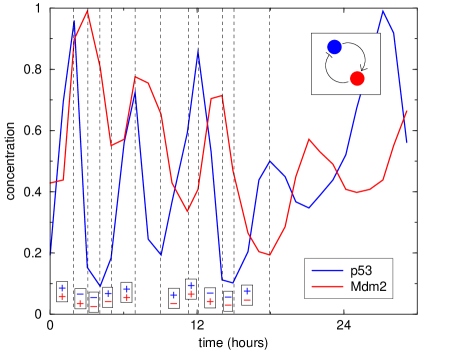
(b)

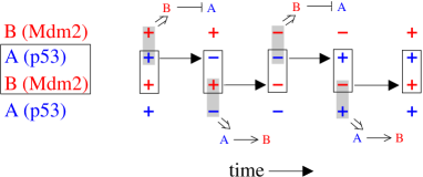
Figure 1: (a) p53-Mdm2 oscillations as recorded in a fluorescence microscopy experiment [7] and the reconstructed symbolic dynamics. Inset shows the negative feedback loop extracted using the algorithm in the text; the process is shown in (b). Here, and in subsequent figures, ordinary arrows represent activation, while barred arrows represent repression.

As an example, consider the p53-Mdmd2 oscillations observed in single-cell fluorescence experiments, shown in Fig. 1a. One could ask, what causes the fluctuations in the amplitude of the observed oscillations? Are they caused by an underlying chaotic dynamics, by noise due to interaction with other proteins or by time-delay effects? Even if there are rigorous time-series techniques to answer to this question [21], they are unlikely to give a conclusive answer because of the low statistics.

Nevertheless, the oscillations in Fig. 1a contain precious information about the real system: notice that the time order of the maxima and minima of the concentrations is always the same (where it is possible to discriminate the sequence). In this paper we show that these sequences have a precise pattern for a large class of deterministic, non-time-delayed models of negative feedback loops, meaning that they can be used to deduce the precise order of activators and repressors in the feedback loop generating the time series. We have devised a simple algorithm for doing this which is described in the next section. The mathematical basis for the algorithm is laid out in the subsequent two sections. In the final section, we apply our algorithm to reconstruct the feedback loop from oscillating time series of two more biological systems; the examples also clarify the the scope and limitations of the algorithm.

Extracting the feedback loop

As mentioned above, the time series in Fig. 1a shows a fixed order of maxima and minima of the concentrations. We can investigate this pattern by dividing the dataset into intervals whose ends are determined by the occurrence of an extremal value (maximum or minimum) of a variable. In each of these intervals, marked by vertical dotted lines in Fig. 1a, each variable shows an unchanging trend, either increasing or decreasing with time. We can therefore uniquely associate to each interval a “symbol” of the form $(+,-,+,\ldots)$, containing one sign for each variable, with a ‘$+$’ meaning that that variable is increasing and a ‘$-$’ meaning it is decreasing. In Fig. 1, each box corresponds to one such symbol (for convenience the signs are arranged vertically in all figures, but horizontally in the text). Thus, the continuous time series is converted into a discrete sequence of symbols, which we term the “symbolic dynamics” [22]. The algorithm listed below can then determine whether the sequence is consistent with the dynamics of a single negative feedback loop, and if so, the precise order of activators and repressors in that loop.

The algorithm

1. List the order in which the maxima and minima of the variables occur. E.g., in Fig. 1a, the order is p53 max, Mdm2 max, p53 min, Mdmd2 min, p53 max, Mdm2 max …

2. If the variables occur in this list in an unchanging cyclic order, then this fixes the order of species in the loop, i.e., a variable activates or represses the one immediately following it in the list. Otherwise, a single negative feedback loop is inconsistent with the time series.

3. Construct the symbolic dynamics for the time series, with +/- symbols listed in the order obtained in step 2.

4. If the symbolic dynamics is not periodic, a single negative feedback loop is inconsistent with the time series. Otherwise, start with any variable and the one pointing to it (say, variables B and A) and note the steps where B changes sign. If at the previous step (before B changed), A had the same sign as B then A represses B, else it activates B (see Fig. 1b).

5. This procedure is repeated for each variable to obtain the effect of the preceding variable. E.g., in Fig. 1 we conclude that p53 activates Mdm2, and Mdm2 represses p53. If the various sign changes of any variable give inconsistent conclusions, then a single negative feedback loop is inconsistent with the time series.

6. If the number of repressors in the loop is even, then a single negative feedback loop is inconsistent with the time series.

For p53-Mdm2 oscillations, there are only two possibilities for a single negative feedback loop involving only these two. Either p53 activates Mdm2 which represses p53, or p53 represses Mdm2 which activates p53. The above algorithm applied to Fig. 1a picks out the former, for which experimental evidence already existed [23] (discussed further in the “Examples” section). This is a particularly simple case, as it involves only two variables. Our algorithm aids model selection much more when there are more than two variables involved, as shown in the two other examples discussed in the final section of the paper. First, we establish the mathematical basis for this algorithm.

Figure 2: Examples of negative feedback loops: a) The simplest case consisting of one activator and one repressor. b) a 3-repressor loop, c) a general loop with $N$ variables and an odd number of repressors.

A general class of negative feedback loops

Consider a feedback loop composed of an arbitrary number, $N$, of nodes, where each node can be either an activator or a repressor (see Fig. 2c). Nodes could be genes, proteins, metabolites or any other chemical species which could, directly or indirectly, activate or repress other nodes in the system. The equations we study are of the form:

$$\frac{dx_{i}}{dt}=g_{i}^{(A,R)}(x_{i},x_{i-1})\qquad i=1\ldots N.$$ (1)

$x_{i}$ is a dynamical variable associated to node $i$, e.g., the concentration of the chemical species $i$, or the expression level of gene $i$. Henceforth, we will call $i$ a chemical species and $x_{i}$ its concentration. The vector field, whose components are $g_{i}(x,y)$, contains all the basal production, degradation, and possibly self-catalytic terms, and specifies the interaction between variables. We denote explicitly with the superscript that each species $i$ is either activated (A) or repressed (R) by the species $i-1$ immediately preceding it in the loop. We allow for heterogeneity, meaning that the different species can be characterized by different production and degradation rates, and different interaction strengths, i.e., different functions $g_{i}$ for each $i$. The functions can also be nonlinear. For instance, one way of implementing the 3-repressor loop in Fig. 2b would be:

$$\frac{dx_{i}}{dt}=c-\gamma x_{i}+\alpha\frac{1}{1+(x_{i-1}/K)^{h}},$$ (2)

for $i=1,2,3$ (with $i=0$ the same as $i=3$). These equations model the basal production of each protein ($c$), the uniform dilution of each proteins by cell growth ($\gamma$) and the production of each protein ($\alpha$) that is repressed by the one behind it in the circuit. The repression we have chosen to be of a standard Michaelis-Menten form, with half-maximum at $K$. The Hill coefficient, $h$, models the cooperative prevention of transcription by $h$ molecules of $i-1$ binding at the promoter of $i$. This is a simplified version of the repressilator [24].

This example simply provides a single illustration of possible $g_{i}$ functions. In fact, we do not constrain the $g_{i}$ to be like eq. 2. The only restrictions we put on the functions $g_{i}$ are the following two conditions:

1. All trajectories should be bounded and persistent, meaning that all the concentrations should stay positive and finite in the time evolution.

2. Monotonicity: all the $g_{i}(x,y)$s have to be monotonically decreasing functions of the first argument. Moreover, the $g^{R}(x,y)$ are decreasing functions of the second argument, while the $g^{A}(x,y)$ are increasing functions of the second argument.

Condition 1 is imposed to ensure that concentrations of the species are well defined and cannot grow infinitely, a biologically plausible constraint: typically for regulatory networks, $g_{i}$ is bounded above (i.e., there is a maximum possible rate of production) and is dominated by the degradation terms for sufficiently large concentrations, thus ensuring condition 1. Condition 2 implies that activators of a specific process are activators at all concentrations (and similarly for repressors). In other words, we exclude regulation like CI in lambda phage which can activate the $P_{\mathrm{RM}}$ promoter at low concentrations, but repress it at high concentrations [25]. Another example is the galactose regulator GalR, which at high concentrations of galactose is an activator of the promoter galP2 but in the absence of galactose forms a DNA loop, in which state galP2 is completely repressed [26]. Such examples are, however, relatively rare and we exclude them from the class of networks we study.

The monotonicity condition can be used to prove that if the number of repressors in the loop is even there can be multiple fixed points. This is necessary for bistable or multistable systems, as previously analyzed in [27]. In the following we focus on the case of an odd number of repressors, i.e., negative feedback. Then, as shown in supplementary material, there is one and only one fixed point. Further, a linear stability analysis shows that the transition to instability is necessarily a Hopf bifurcation, which implies that near the transition point there exists a periodic orbit (see supplementary material). However, this stability analysis allows one to study the dynamics only locally, both in the phase space, i.e., close to the fixed point, and in parameter space, i.e., close to the bifurcation value. In the next section, we show that in general, whether the fixed point is stable or unstable, there are restrictions on the trajectory of the system.

Symbolic dynamics

Our argument is the direct consequence of how the nullclines, i.e., the $N$ manifolds defined by the equations $g_{i}(x_{i},x_{i-1})=0$, partition the phase space (the positive orthant $x_{i}>0\ \ \forall i$.) Each nullcline separates two fully connected regions, one in which the $i$th component of the field, $g_{i}$, is positive and one in which it is negative. Furthermore, all these manifolds have exactly one point in common, the unique fixed point ${\mathbf{x}}^{*}$. The phase space is thus the union of $2^{N}$ sectors, each characterized by the signs of the components of the field. These sectors correspond precisely to the symbols $(+,-,-,+,\ldots,-)$ defined previously.

Notice that there cannot be an attractor entirely contained in the interior of a sector because the field does not change sign, the trajectory is bounded and there is only one fixed point. Thus, either the trajectory of the system spirals in towards a stable fixed point, or, if the fixed point is unstable, it will keep crossing from one sector to another indefinitely. In the first case, the symbolic dynamics is a finite sequence of symbols, which ends when the trajectory stops crossing sector boundaries. In the latter case, it will be an infinite sequence of symbols. In either case, adjacent symbols in the sequence will differ by only one sign change.

The key point of our argument is that any of the boundaries can be crossed in just one specific direction, due to the monotonicity of the functions $g_{i}(x_{i},x_{i-1})$. This means that not all possible sign changes are allowed. In Fig. 3, we illustrate this using the example of the 2-species negative feedback loop of Fig. 2a, one repressor and one activator. Fig. 3b shows the only 4 transitions possible in this system. Thus, starting from any initial condition, the symbolic dynamics will follow the order shown in Fig. 3b until the trajectory converges to the stable fixed point and there are no further sign changes. This example gives a good pictorial idea of the fact that the nullclines behave like one-way doors.

Figure 3: (a) Schematic diagram of the phase-space of the 2-variable negative feedback loop of Fig. 2a. Solid lines show the two nullclines, which intersect and divide the space into four sectors, labelled by the signs of $g_{1}$ (top sign) and $g_{2}$ (bottom) in that sector. Arrows on the nullclines show the local direction of the vector field, which determines the direction in which the nullcline can be crossed by a trajectory. The dotted line is an example trajectory which follows these rules, while spiralling in towards the stable fixed point. (b) The allowed transitions for moving from one sector to another. The symbolic dynamics of any trajectory has to be consistent with these rules.

In the general $N$-species case, the same phenomenon occurs, with the symbolic dynamics obeying the following rules (see supplementary material for more information).

• If the variable $(i-1)$ represses $i$, the nullcline $i$ can be crossed if $g_{i}$ and $g_{i-1}$ have the same sign.

• If the variable $(i-1)$ activates $i$, the nullcline $i$ can be crossed if $g_{i}$ and $g_{i-1}$ have opposite signs.

To emphasise the point further, the direction in which the nullcline $g_{i}=0$ can be crossed at a given point depends on the position of that point relative to only one other nullcline, $g_{i-1}=0$. It does not depend on any other nullcline. In simple words, the rules encode the fact that an increasing activator can make the affected concentration increase (but not decrease), while an increasing repressor can make the affected concentration decrease (but not increase). Note that the allowed transitions apply to any trajectory, even transients. Thus, if one is analysing oscillatory time series it doesn’t matter whether the oscillations are sustained, or the measurement is of transients or damped oscillations.

To determine the general scenario which is compatible with these rules, consider that when a nullcline is crossed, the symbolic dynamics makes a transition between two states differing by just a single sign. We say that there is a mismatch between two adjacent signs if the nullcline depending on these two variables can be crossed according to the rules defined above. The effect of crossing the nullcline $i$ is to remove the mismatch between $i$ and $i-1$. If there was also a mismatch between $i$ and $i+1$, it too is removed, otherwise it is created. For a negative feedback loop, we can show that the number of mismatches has to be odd, and cannot increase.

Now consider what happens if the fixed point is unstable. If there is just one mismatch, it can only keep traveling around the loop, in the direction of the loop arrows. This means that the symbolic trajectory is periodic of period $N$. In the general case we can visualise the symbolic dynamics as several mismatches traveling around the loop in the same direction. Whenever two mismatches “hit” each other, they annihilate. Eventually the number of mismatches will reach some limit, where each mismatch stays safely distant from the others. The length of the loop limits how many mismatches can, in principle, coexist; for example, only one mismatch can survive if $N<4$. In practice, even in long loops, it is likely that only one mismatch survives and we will restrict to this case in the following.

An interesting consequence of this periodicity is that any of the $N$ nullclines defines a Poincaré map for the dynamical system. Periodic oscillations in the symbolic dynamics translate into a stable periodic orbit if the dynamics on the Poincaré map reaches a fixed point, or into chaotic oscillations if the dynamics on the Poincaré map is chaotic.

Whether the orbits are chaotic or not we have proven, for this general class of systems, that when the fixed point is unstable, the dynamics is oscillatory with well defined properties. For example, each of the concentrations has exactly one maximum and one minimum during a time period of the symbolic dynamics, and the fact that the mismatch travels in the direction of the feedback loop implies that the sequence of maxima and minima has to follow the order of the species in the loop. From the particular order observed it is also possible to argue which species acts as an activator and which as a repressor. Furthermore, the observation of a time series which is incompatible with the symbolic dynamics rules allows one to exclude a dynamics of the form of eq. (1), generally suggesting a topology more complicated than a simple feedback loop or more subtle effects like time delays and non-monotonic regulation. The algorithm described previously is a straightforward consequence of these rules.

Notice that our method works even if one does not measure the time series of all the species belonging to the loop. The algorithm gives a coherent conclusion about the overall sign between the variables: for example, a variable A will appear as an activator of a variable B if there is an even number of “unobserved” repressing links between them (see supplementary material). The following examples will further clarify these points.

Examples

We now apply the above ideas to extract information about the loop structure from experimentally observed time series of three systems: p53-Mdm2 oscillations in mammalian cells, circadian expression of kai genes in Synechocystis cyanobacteria, and cyclic binding of protein cofactors with DNA at the estrogen-sensitive pS2 promoter in human breast cancer cells.

Our first example is the well-known p53-Mdm2 negative feedback loop, already discussed in the introduction. The tumor suppressor protein, p53, is a transcription factor that affects the expression of a large number of genes including several involved in cell cycle arrest and apoptosis, while Mdm2 is an important regulator of p53 activity [28]. For the oscillating concentrations of p53 and Mdm2 in Fig. 1, in a couple of cases there is some ambiguity about the order of maxima and minima. However, the pattern is clarified by comparing two separate time intervals in which the symbolic sequence is unambiguous. Notice that both regions exhibit the same periodic symbolic sequence. According to the rules we stated in the previous section, this sequence is allowed if p53 activates Mdm2 and Mdm2 represses p53. This is completely consistent with independent experimental knowledge of the system. p53 activates transcription of the mdm2 gene [23]. Mdm2, once produced, binds to p53 preventing it from acting as a transcription factor, and subsequently ubiquitinates it, which enhances its proteolytic breakdown [23]. Thus, Mdm2 is a repressor of p53. Therefore, we conclude: (i) the observed oscillations are consistent with a dynamics of the form of eq. (1), (ii) however, for this there must be at least one other unobserved species taking part in the loop, since the fixed point is always stable for $N=2$. Indeed, several three variable models of p53-Mdmd2 oscillations have been examined, which assume the third variable to be either an Mdm2 precurser (e.g., Mdm2 mRNA) or a third protein which interacts with p53 or Mdm2 [7]. Of course, it is hard to say at this level if a simple, deterministic negative feedback loop is a good model for this specific system. For example, the same sequences of symbols could be observed in a time-delay model [11]. In addition, experiments suggest the presence of at least 10 feedback loops involving p53 [29]. It is also nontrivial to assess whether the aperiodicity of the trajectory is due to internal mechanisms (chaos, time delays), or to interaction with other proteins. Still, we can conclude that a model like eq. (1) is a good candidate for a zero-order model, being simple and reproducing correctly the qualitative behavior of the components with the correct interaction signs.

The next example involves circadian oscillations of gene expression in cyanobacteria. Cyanobacteria are the only bacterial species with a circadian clock and several of their cellular functions appear to be under circadian control [4]. In Synechococcus elongatus a cluster of three genes, kaiA,B,C, were found to be essential: deletion of any of these genes eliminated the oscillations [30]. Fig. 4a shows circadian rhythms in the expression levels of genes coding for homologues of the KaiA,B,C proteins in one Synechocystis strain. The symbolic dynamics is consistent with a three-variable feedback loop (Fig. 4a, inset), where kaiA activates kaiC1, which represses kaiB3, which, in turn, activates kaiA. The first two of these predicted interactions exist in Synechococcus [30], while the third is a new prediction for how kaiA is brought into the loop. Note that our analysis only provides the sign of this interaction. It does not reveal the molecular mechanism of the interaction, nor whether the interaction is direct or through intermediate steps.

(a)

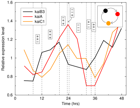
(b)

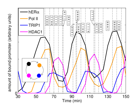
Figure 4: (a) Circadian rhythms of three kai genes in a Synechocystis cyanobacterial strain (data from ref. [31]). (b) Periodic binding of four proteins to the pS2 promoter following addition of estradiol (data from ref. [33], based on ref. [32]). In each case the corresponding symbolic dynamics is also shown, with symbols in the same order as the legend (where maxima/minima of two variables occur very close we have exaggerated the separation between the dotted lines for visual clarity). The insets shows the topology deduced from the symbolic dynamics.

Finally, we consider the cyclic binding of cofactors to the estrogen-sensitive pS2 promoter. A coordinated sequence of binding and unbinding events modifies the DNA packing and nucleosome structure to enable transcription to proceed [32]. This is a case where no model exists and not all the proteins involved have been identified. Our method is particularly suited for such a case, because it does not matter if the dynamics of only a subset of the proteins involved is available. Ref. [32] measured the temporal dynamics of binding of several proteins at the pS2 promoter using ChIP assays. Fig. 4b shows oscillations in the binding of 4 proteins, after the addition of estradiol. ER, estradiol receptor, binds estradiol and is required for initiating transcription. Pol II is the RNA polymerase that transcribes the gene. TRIP1 is a component of the APIS proteasome subunit, while HDAC1 is involved in deacetylation of histones [32]. The symbolic dynamics is consistent with the model shown in Fig. 4b, inset. Notice that in this case, each variable measures the amount of bound protein at the pS2 promoter (albeit in arbitrary units, which are different for each protein). The predicted links indicate how a bound protein affects the probability of binding (or of remaining bound) of another one in the sequence. For example, the link from ER to Pol II indicates that ER, when bound at the promoter, increases the recruitment probability of Pol II. Ref. [33] models the dynamics of Fig. 4b using a positive feedback loop, requiring over 200 intermediate steps, which has only activating links. Our analysis predicts the existence of a repressive link between HDAC1 and ER. One could imagine this repression as a result of a change in the conformational state of the DNA or histones, or the blocking of a binding site for ER at the promoter. However, we emphasise again that our analysis does not give any information about the molecular mechanism for this repression or whether there are intermediate steps. The analysis does suggest that, for this system, a negative feedback loop is a plausible hypothesis as the cause of oscillations.

Supplementary Material for “Oscillation patterns in negative feedback loops”

Fixed point analysis

In this section we study the fixed point properties of a feedback loop composed of an arbitrary number, $N$, of nodes whose dynamics is given by Eq. (1) in the main text, which we repeat here:

$$\frac{dx_{i}}{dt}=g_{i}^{(A,R)}(x_{i},x_{i-1})\qquad i=1\ldots N.$$ (3)

Our analysis proceeds by noting that, using the monotonicity condition, we can write explicit functional relations between neighboring variables in the steady state (when $dx_{i}/dt=0$):

$$g_{i}^{(A,R)}(x_{i}^{*},x_{i-1}^{*})=0\quad\Rightarrow\quad x_{i}^{*}=f_{i}^{(A,R)}(x_{i-1}^{*})$$ (4)

Notice that the functions $f_{i}$ have the same monotonicity properties as the $g_{i}$s with respect to the second argument (for this it is necessary that $g_{i}(x,y)$ be a monotonically decreasing function of $x$). By iterative substitution, we obtain:

$$x_{i}^{*}=f_{i}(x^{*}_{i-1})=f_{i}(f_{i-1}(x^{*}_{i-2}))=\ldots=$$

$$=f_{i}\circ f_{i-1}\circ f_{i-2}\circ\ldots\circ f_{i+1}(x^{*}_{i})\equiv F_{i}(x^{*}_{i})$$ (5)

where $\circ$ denotes convolution of functions. Here, we introduced the function $F_{i}(x)$, which quantifies how the species $i$ interacts with itself by transmitting signals along the loop. Notice also that if Eq.(Fixed point analysis) holds for one value of $i$, then it holds for any $i$, since it is sufficient to apply $f_{i+1}()$ on both sides to obtain the equation for $x_{i+1}^{*}$ and so on. For feedback loops, much useful information can be obtained from the properties of $F_{i}(x)$. Firstly, by applying the chain rule, we obtain the slope of $F_{i}(x)$ at $x$: $F_{i}^{\prime}(x)=\prod_{j}f_{j}^{\prime}(x_{j})|_{x_{i}=x}$. The r.h.s is always greater (less) than zero if the number of repressors present in the loop is even (odd). In the former case, there can be multiple fixed points, i.e., this is a necessary condition for multistability. On the other hand, when there are an odd number of repressors, then $F_{i}(x)$ is positive and monotonically decreasing, meaning that there is one and only one solution to the fixed point equation $x^{*}_{i}=F_{i}(x_{i}^{*})$. The system of equations (1) has one unique fixed point, which we denote ${\bf x}^{*}$. To perform the stability analysis, we write the characteristic polynomial evaluated at this point:

$$\prod_{i}\left[\lambda-\partial_{x}g_{i}(x,y)|_{x=x^{*}}\right]=\prod_{i}\partial_{y}g_{i}(x,y)|_{x=x^{*}}.$$ (6)

The above equation can be greatly simplified using the relation $F^{\prime}(x)=\prod_{i}\partial_{y}g_{i}(x,y)/\partial_{x}g_{i}(x,y)$, which is a consequence of the implicit function theorem and the chain rule. One then obtains the following equation:

$$\prod_{i=1}^{N}\left(\frac{\lambda}{h_{i}}+1\right)=F^{\prime}(x^{*})$$ (7)

where the $h_{i}=-\partial_{x}g_{i}(x_{i},x_{i=1})|_{x^{*}}$ are the degradation rates at the fixed point. Notice that, because $F^{\prime}(x)$ is always negative in a negative feedback loop, all coefficients of the characteristic polynomial are non-negative, hence it can not have real positive roots. This means that the destabilization of the fixed point can only occur via a Hopf bifurcation, i.e. with two complex conjugate eigenvalues crossing into the positive real half-plane.

In the simple case in which all the degradation rates are equal and unchanging (i.e, $h_{i}=\gamma$, a constant) the roots of the polynomial (7) in the complex plane are the vertices of a polygon centered on $-\gamma$ with a radius $|F^{\prime}|$ as sketched in Fig. 5.

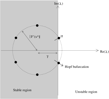
Figure 5: Sketch of the Hopf bifurcation in the eigenvalue complex plane, in the case in which all the degradation rates are equal to a constant $\gamma$.

Therefore, the fixed point will remain stable as long as

$$|F^{\prime}(x^{*})|\cos(\pi/N)<\gamma.$$ (8)

In this case, Hopf’s theorem (see e.g. [1]) ensures the existence of a periodic orbit close to the transition value, whose period is:

$$T=2\pi/Im(\lambda)$$ (9)

which, in the simple case of equal degradation timescales, becomes $T=2\pi/[|F^{\prime}(x^{*})|\cdot\sin(\pi/N)]$. Notice that the Hopf theorem does not ensure that the orbit is stable; however, since the system is bounded and there are no other fixed points, we expect the orbit to be attracting, at least close to the transition point.

Now we apply these ideas to the 3-repressor example discussed in the main text:

$$\frac{dx_{i}}{dt}=c-\gamma x_{i}+\alpha\frac{1}{1+(x_{i-1}/K_{i})^{h}}\qquad i=1\ldots 3.$$ (10)

The coordinates of the fixed point are all equal due to symmetry. We denote by $x^{*}$ the solution to the equation $\gamma x=c+\alpha/(1+(x/K)^{h})$. Then the characteristic polynomial is simply:

$$(\lambda+\gamma)^{3}=-\left(\frac{\alpha}{1+(x^{*}/K_{i})^{h}}\right)^{3}$$ (11)

Notice, that this can be written as:

$$\left(\frac{\lambda}{\gamma}+1\right)^{3}=F^{\prime}(x^{*})$$ (12)

The stability condition is then:

$$|F^{\prime}(x^{*})|\cos(\pi/3)<\gamma.$$ (13)

Fig. 6a shows that $|F^{\prime}|$ satisfies this condition for $h=2$ (black curve) but not for $h=4$ (red curve), when the other parameters are kept fixed at the values $\alpha=3.0,~{}c=0.1,~{}K=1,~{}\gamma=1$. Consequently, for $h=2$ the trajectory converges to a stable fixed point, whereas it converges to a stable limit cycle for $h=4$, as shown in the inset of Fig. 6a.

(a) (b)  

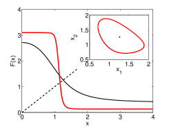
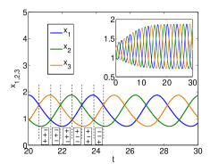
Figure 6: A simple genetic oscillator described by eq. (10). (a) Plot of $F_{1}(x)$ for $h=2$ (black solid curve) and $h=4$ (red curve). Other parameters are kept fixed: $\alpha=3.0,~{}c=0.1,~{}K=1,~{}\gamma=1$. The fixed point value of $x_{1}$ in each case lies at the intersection of the curves with the dotted line. Inset shows the corresponding trajectories in the $x_{1}x_{2}$ plane. (b) Time evolution of $x_{1,2,3}$ for the $h=4$ case after a stable limit cycle is reached (inset shows a longer time plot including the transient). Also shown is the symbolic dynamics for this time evolution.

Symbolic dynamics

In this section we give the mathematical details of the section “Symbolic dynamics” in the paper. This section is organized in the same order as in the main text and we will repeat the statements made there in a mathematically more rigorous way.

Let us use $\Gamma$ to denote the phase space, i.e. the positive orthant:

$$\Gamma=\{x_{i}>0\}\qquad\forall i=1\ldots N.$$ (14)

In the systems in which trajectories are bounded only when the concentrations do not grow more than some maximum value (this is the case of saturated degradation), all the following considerations still hold, with the prescription of taking $\Gamma$ to be the subset of the positive orthant in which the concentrations are bounded.

Our goal is to describe how the space $\Gamma$ is partitioned by the $N$ nullclines $\mu_{i}$ defined by $g_{i}(x_{i},x_{i-1})=0$. The properties we are about to state are all consequences of the monotonicity of the functions $g_{i}(x_{i},x_{i-1})=0$, the constraint of having bounded and persistent orbits and the existence of a unique fixed point $\mathbf{x}^{*}$.

It is worth remarking here that the existence of a fixed point is more a consequence of the boundedness condition, rather than the monotonicity condition. Indeed, if the function $f_{i}(x_{i-1})$ and $f_{i-1}^{-1}(x_{i-1})$ (see Eq.(2)) have independent support, they will obviously have no intersection. But in this case the system will not be persistent: persistence requires that $\lim_{x\rightarrow 0}g(x,y)>0\ \forall y$ and boundedness requires that $\lim_{x\rightarrow\infty}g(x,y)<0\ \forall y$; in this case, the nullclines have to cross. This fact is crucial also for the other considerations in this section on the phase space portrait. Actually the existence of a fixed point could have been demonstrated using only the boundedness and persistence hypothesis by means of Brouwer’s fixed point theorem (see e.g. [2]).

Returning to the partitioning of $\Gamma$, the first important property is that any nullcline divides $\Gamma$ into two simply connected sets, one in which $g_{i}(\mathbf{x})>0$ and one in which $g_{i}(\mathbf{x})<0$. Notice also that these manifolds cannot be tangent at the fixed point because of monotonicity and since they can depend on at most one common variable. All these properties imply that the $\Gamma$ space is partitioned by the nullclines into $2^{N}$ simply connected subsets, which we called “sectors” in the main text. In each of these sectors every component of the vector field has a definite, unchanging, sign. We use here the same notation as the main text and denote each of these sectors with a sign vector like $(+,-,-....+)$. As stated in the paper, the uniqueness of the fixed point and the fact that the field has a constant sign inside a sector allows one to exclude the possibility of an attractor entirely contained within a sector. In the rest of this section, we discuss the case in which the fixed point is unstable. Since we assume that trajectories are bounded, starting from a sector the trajectory has to leave it by crossing one of the $N$ boundaries. We show in Fig. 3 in the main text that a given boundary $g_{i}=0$ can be crossed in just one direction using a simple, two dimensional example. We show here a three dimensional example of how a stable periodic orbit crosses the nullclines. We consider the following model, consisting of one repressor and two activators (this is similar to one of the 3-variable models of the p53 system discussed in [3]):

$$dx_{1}/dt = s-x_{3}x_{1}/(K+x_{1})$$

$$dx_{2}/dt = x_{1}^{2}-x_{2}$$

$$dx_{3}/dt = x_{2}-x_{3}$$ (15)

This system of equations has a stable periodic orbit as an attractor for parameters values $s=30$, $K=.1$. The phase space portrait, together with a plot of the nullclines, is shown in Fig.(7).

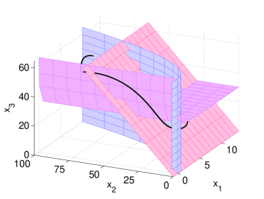
Figure 7: Stable periodic orbit and plot of the nullclines for a model of the p53 system, defined by the system of equations (Symbolic dynamics).

Indeed, due to the fact that a given nullcline $g_{i}=0$ is “flat” in all directions perpendicular to $x_{i}$ and $x_{i-1}$, no new topological features appear in the higher dimensional cases; in particular the direction in which this nullcline can be crossed depends only on the sign of $g_{i}$ and $g_{i-1}$, and never on any other nullcline. This directly follows from the fact that all the manifolds $\mu_{i}\cap\mu_{j}$ (intersections of a pair of nullclines) are simply connected; it is easy use the function $f_{i}(x)$ defined in Eq.(2) to write an explicit and continuous parameterization of these manifolds. It should be clear at this point that the following fact is true in any dimension $N$: the portion of the nullcline which forms the boundary between two adjacent sectors can only be crossed in one direction.

The above italicised statement directly implies the two transition rules stated in the main text, which we repeat here:

• If the variable $(i-1)$ represses $i$, the nullcline $i$ can be crossed if $g_{i}$ and $g_{i-1}$ have the same sign.

• If the variable $(i-1)$ activates $i$, the nullcline $i$ can be crossed if $g_{i}$ and $g_{i-1}$ have opposite signs.

We associate to a given symbol, or sector, the quantity $H$ defined as the number of boundaries that can be crossed from that sector. Notice that $H=0$ is impossible. For this to happen, the above rules must be violated by every adjacent pair of signs, i.e., the signs on both ends of an activation arrow must be the same, while the two signs on both ends of a repression arrow must be different. As there are an odd number of repressors, this is impossible. Therefore, $1\leq H\leq N$. When the trajectory crosses a nullcline $g_{i}=0$, as a simple consequence of the transition rules, $H$ either stays constant if the nullcline $g_{i+1}$ can be crossed from the new sector, or decreases by two if $g_{i+1}$ cannot be crossed (see Fig. 8). Physically, if we think of a crossable boundary as an unsatisfied bond between sign $i$ and $i-1$ (termed “mismatches” in the main text), $H$ is the number of such mismatches, hence it quantifies the level of “frustration” in the system. The time evolution can then (i) solve two neighboring unsatisfied bonds, or (ii) shift an unsatisfied bond one place to the right, i.e. from $i$ to $i+1$. As a consequence: $H$ can never increase, and it must always be an odd number.

$i-1$ (see Fig 8).

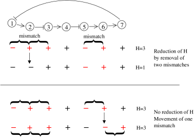
Figure 8: Consequences of crossing a nullcline for the sign vector and the quantity $H$. Upper panel: a sign is changed between two mismatches and, consequently, $H$ decreases by 2. Lower panel: a sign is changed next to just one mismatch. In this case, the mismatch simply moves one step ahead in the loop; the value of $H$ does not change.

We expect the system to end up in a state in which $H=1$ and the unsatisfied bond keeps on moving around the loop in the direction of the arrows. This represents, at the level of symbolic dynamics, a single “signal” traveling around the loop. A direct implication is that the extremal points (maxima or minima) of all variables should appear in the time series in the order in which the species are arranged in the cycle.

This is the simplest scenario and is the only one for $N<4$. What can actually happen for $N\geq 4$ is that $H=3$ can become a stable state, with $3$ different signals traveling along the feedback loop. However, even if there is an attractor with $H=3$, it must anyway coexist with an $H=1$ attractor, since if a trajectory ever starts from, or enters, a sector with $H=1$, it can never return to an $H=3$ sector. Further, the $H=3$ attractor is likely to require some fine tuning of parameters to avoid one mismatch travelling “faster”, catching up and annihilating another one. It is thus likely that any perturbation or noise would bring the system to the “ground state” attractor characterized by $H=1$, and that is the one we expect to observe in biological systems.

Unobserved variables

We conclude by arguing that the presence of unobserved variables does not alter our conclusions. Essentially the rules we stated depend only on the overall sign between two variables and it is irrelevant if there are species in between mediating their interaction. This can be easily shown by considering all the possible cases of an intermediate species being an activator/repressor and being activated/repressed. Then it can be generalized by induction to an arbitrary number of mediators. Since the general demonstration is straightforward, consisting essentially of considering all the possible cases, we show here just one example: the three-repressor loop of the previous section, in which one of the species is unobserved. We write its symbolic dynamics (as in Fig. 6b) by means of the rules we shown and simply cancel the second row:

$$\begin{array}[]{c}x_{1}\\ x_{2}\\ x_{3}\end{array}\left(\begin{array}[]{c}-\\ +\\ -\end{array}\right)\left(\begin{array}[]{c}+\\ +\\ -\end{array}\right)\left(\begin{array}[]{c}+\\ -\\ -\end{array}\right)\left(\begin{array}[]{c}+\\ -\\ +\end{array}\right)\left(\begin{array}[]{c}-\\ -\\ +\end{array}\right)\left(\begin{array}[]{c}-\\ +\\ +\end{array}\right)$$ (37)

$$\longrightarrow\left(\begin{array}[]{c}-\\ -\end{array}\right)\left(\begin{array}[]{c}+\\ -\end{array}\right)\left(\begin{array}[]{c}+\\ +\end{array}\right)\left(\begin{array}[]{c}-\\ +\end{array}\right)\begin{array}[]{c}x_{1}\\ x_{3}\end{array}$$ (48)

The resulting symbolic dynamics is that of a two species loop with one activator and one repressor (like the p53-Mdm2 oscillations in Fig. 1 in the main text). Here, as expected, two repressing links become one activating link if the intermediate species, $x_{2}$, is unobserved.

References

- [1] Massé E. and Arguin M. (2005) Trends Biochem. Sci. 30, 462–468.
- [2] Friedman, N., et al., (2005) PLoS Biol. 3, e238.
- [3] Oppenheim, A. B., Kobiler, O., Stavans, J., Court, D. L. and Adhya, S. (2005) Annu. Rev. Genet. 39, 409–429.
- [4] Golden, S. S., Ishiura, M., Johnson, C. H., Kondo, T. (1997) Annu. Rev. Plant Physiol. Plant Mol. Biol. 48, 327–354.
- [5] Hoffmann, A., Levchenko, A., Scott, M. L. & Baltimore, D. (2002) Science 298, 1241–1245.
- [6] Nelson, D. E., Ihekwaba, A. E. C., Elliott, M., Johnson, J. R., Gibney, C. A., Foreman, B. E., Nelson, G., See, V., Horton, C. A., Spiller, D. G. et al. (2004) Science 306, 704–708.
- [7] Geva-Zatorsky, N et al. (2006) Molecular System Biology 2 doi:10.1038/msb4100068.
- [8] Hirata, H., Yoshiura, S., et al. (2002) Science 298, 840–843.
- [9] Leloup, J.-C & Goldbeter, A. (2003) Proc. Natl. Acad. Sci. (USA) 100, 7051–7056.
- [10] Krishna S., Jensen M. H. and Sneppen K. (2006) Proc. Natl. Acad. Sci. 103, 10840-10845.
- [11] Tiana G., Jensen M.H., Sneppen K. (2004) Eur. J. Phys. B 29(1), 135-140.
- [12] Jensen, M. H., Sneppen, K., Tiana, G. (2003) FEBS Lett. 541, 176–177.
- [13] Chen, L. et al (2004) Phys. Rev. E 70, 011909.
- [14] Nakajima M. et al., (2005) Science 308 414-415.
- [15] Lakin-Thomas P. L. (2006) Journal of biological rhythms 21(2), 83-92.
- [16] Thomas, R. (1981) in Quantum Noise, Springer Series in Synergetics 9, ed. Gardiner, C. W. (Springer, Berlin), pp. 180-193.
- [17] Snoussi, E. H. (1998) J. Biol. Sys. 6, 3-9.
- [18] Gouzé, J. L. (1998) J. Biol. Sys. 6, 11-15.
- [19] Forger D.B. and Peskin C. S. (2005) Proc. Natl. Acad. Sci. 102(2), 321-324.
- [20] Lauzeral, J., Halloy, J., Goldbeter, A. (1997) Proc. Natl. Acad. Sci. (USA) 94, 9153–9158.
- [21] Kantz H. and Schreiber T. (2003) Nonlinear time series analysis, Cambridge University Press.
- [22] Strogatz, S. Nonlinear Dynamics and Chaos, Addison-Wesley, Reading MA, 1994.
- [23] Wu, X., Bayle, J. H., Oldon, D., Levine, A. J. (1993) Genes Dev. 7, 1126–1132.
- [24] Elowitz M. B. and Leibler S. (2000) Nature 403, 335-338.
- [25] Dodd, I. B., Perkins, A. J., Tsemitsidis, D., Egan, J. B. (2001) Genes Dev. 15, 3013–3022.
- [26] Semsey S, Virnik K, Adhya S. (2006) J Mol Biol. 358, 355–63.
- [27] Angeli D., Ferrell J. E., and Sontag E.D. (2004) Proc. Natl. Acad. Sci. 101(7), 1822-1827.
- [28] Levine A.J., Hu W. and Feng Z., Cell Death and Differentiation (2006) 13, 1027-1036.
- [29] Harris S. L. and Levine H. J., (2005) Oncogene 24, 2899-2908.
- [30] M. Ishiura et al. (1998), Science 281, 1519-1523.
- [31] Ken-ichi Kucho et al., (2005), Journ. Bacteriol. 187(6), 2190-2199.
- [32] Métivier R. et al. (2003) Cell, 115 751-763.
- [33] Lemaire V. et al., (2006) Phys. Rev. Lett. 96, 198102.

References

- [1] Murray J.D. (2004) Mathematical Biology, Springer.
- [2] J Hofbauer J., Sigmund, K. (1998) Evolutionary games and population dynamics, Cambridge University Press.
- [3] Geva-Zatorsky, N. et al. (2006) Molecular System Biology 2 doi:10.1038/msb4100068.