Towards the Human Genotope

Abstract

The human genotope is the convex hull of all allele frequency vectors that can be obtained from the genotypes present in the human population. In this paper we take a few initial steps towards a description of this object, which may be fundamental for future population based genetics studies. Here we use data from the HapMap Project, restricted to two ENCODE regions, to study a subpolytope of the human genotope. We study three different approaches for obtaining informative low-dimensional projections of this subpolytope. The projections are specified by projection onto few tag SNPs, principal component analysis, and archetypal analysis. We describe the application of our geometric approach to identifying structure in populations based on single nucleotide polymorphisms.

1 Introduction

The HapMap Project [12] is an international effort to identify the genetic variation in the human population. This includes the identification of all single nucleotide polymorphisms (SNPs) arising in human populations. In the first major published study [12], approximately ten million SNPs are described throughout the human genome, derived from the genotypes of 269 individuals from four populations. A crucial component of the project has involved the comprehensive detection of all SNPs in ten $500$kb regions of the human genome. The ten regions were selected from targets studied by the ENCODE project [8], whose goal is to annotate 1% of the human genome. Thus, while the haplotype map of the human genome is not complete, substantial progress has been made to date, and there is every reason to expect a completed map in the near future.

The characterization of genetic variation in the human population is only a first step towards the fundamental goal of relating phenotypes to genotypes. While in principle every SNP may contribute individually to a phenotype, interactions among loci are common. Furthermore, the problem of identifying relevant SNPs, and understanding the interactions among them, is confounded by the vast number of SNPs in the genome. These issues make it non-trivial to perform association mapping, in which phenotypes are mapped by analyzing genotypes of cases and controls. Fortunately, this problem is ameliorated by two factors. First, the number of individuals in the human population is far smaller than the number of possible haplotypes, so that even if every individual on earth were genotyped, the description of the data would not involve all possible haplotypes. Secondly, there is a lot of linkage disequilibrium (LD), which describes the situation in which some combinations of alleles occur more or less frequently in a population than would be expected by the overall frequency of the alleles in the population. Thus, “informative” SNPs, also known as tag SNPs, can be identified and used to simplify the measurement of variation, and also to reduce the number of loci that need to be considered for association mapping.

The data produced by the HapMap project are useful to understand these issues. By way of example, we consider ENCODE region ENr131. This is a $500064$-base region from chromosome 2. The HapMap project has revealed that there are $2995$ SNPs in the region, meaning that even though there are $500064$ bases, the genomes of any two individuals differ in at most $2995$ sites. These sites typically contain one of two possible alleles, so a human haplotype is described by a binary vector of length $2995$, and a genotype by a vector of length $2995$ whose entries are either $0,1$ or $2$. A $0$ or $2$ indicates that the two haplotypes agree (homozygous), and specifies the allele, and a $1$ indicates disagreement (heterozygous). For our analysis, it is essential that $0$ and $2$ are the homozygotes. This encoding differs from the standard encoding where $0$ and $1$ are homozygotes, and $2$ is the heterozygote (see, e.g., [13]).

In general, a genotype is a vector of length $n$ whose elements are from the alphabet $\{0,1,2\}$. The genotypes for a population of $k$ individuals form a matrix of size $k\times n$. In the case of ENr131, the HapMap project genotyped $1910$ of the $2995$ SNPs in 269 individuals, resulting in a $269\times 1910$ matrix. In fact, it is possible to reduce the number of SNPs that need to be considered in an association mapping study by a factor of 10 by selecting tag SNPs.

The notion of a genotope was introduced in [1] and further developed in [2, 11]. A genotope is the convex hull of all possible genotypes in a population. The regular triangulations of the genotope describe the possible epistatic interactions among the loci. These objects are fundamental for analyzing linkage disequilibrium. For example, the sign of the standard measure of LD for a pair of loci [6] corresponds to one of the two triangulations of the respective genotope (the square). For the data to be examined in this paper, the genotope is the convex hull of $k$ points in $\{0,1,2\}^{n}$, so it is a subpolytope of the $n$-dimensional cube with side length two. In Section 2 we review the relevant mathematical theory and we discuss the meaning of the genotope for population genetics.

The human genotope is the convex hull of about $\,k=6.5\cdot 10^{9}\,$ points, one for each individual in the human population, and the ambient dimension $n$ is bounded above by the number of all SNPs. What can currently be derived from the HapMap data is a subpolytope of the human genotope which is the convex hull of only $k=269$ points, one for each sequenced individual. In this paper we also restrict our attention to two specific ENCODE regions, so that the number $n$ of informative SNPs is on the order of hundreds. We refer to the resulting subpolytopes as the ENCODE genotopes.

In Sections 4-6 we study several different low-dimensional projections of the ENCODE genotopes. These projections are chosen in a statistically meaningful manner, and we argue that the low-dimensional polytopes are a useful geometric representation of the data. In Section 4 we apply Principal Component Analysis (PCA) to determine the most significant projections of our data. We compute the image of the ENCODE genotopes under projection into the six most significant PCA directions. These projections reveal the population structure of the HapMap genotypes in a manner consistent with [15]. We then contrast PCA projections with low-dimensional projections based on tag SNPs. The resulting polytope data are presented in Section 5. This geometric analysis suggests a new statistical test, the volume criterion, for identifying informative SNPs.

In Section 6 we apply a statistical method which is less well-known than PCA but possibly more informative in the population genetics context. Archetypal analysis was introduced by Cutler and Breiman [4] for identifying a small collection of $\ell$ archetypes from $k$ given data points. We apply this method to our $k=269$ genotypes. The archetypes are either genotypes or mixtures of genotypes, so their convex hull is a polytope with $\ell$ vertices inside an ENCODE genotope. We call it the $\ell$-th archetope. Its defining property is that the total least squares error is minimal when each genotype is replaced by its nearest mixture of archetypes. We compute various archetopes and explain how these may be useful for designing genetic studies.

Our studies are preliminary and merely foreshadow the possibilities for a geometric organization of the large amount of genotype data that are currently being produced. We believe that low-dimensional projections of genotopes will be useful for correctly quantifying population structure variation, and also for studying interaction. Our results demonstrate the feasibility of computing low-dimensional projections of genotopes, and our analysis of the HapMap data provides a first step towards the construction of the human genotope.

2 The Human Genotope

The geometric concept of a genotope was introduced in [1] for studying epistasis and shapes of fitness landscapes. This model was applied in [2] to fitness data in E. coli, and its relevance for human genetics was demonstrated in [11].

We briefly review the mathematical setup in [1] but with emphasis on diploids rather than haploids. We consider $n$ genetic loci each of which is a diploid locus with alleles $0,1,2$. A $0$ or $2$ indicates that the two haplotypes agree, and specifies the allele, and a $1$ indicates disagreement. The connection to the classical genetics notation, used to discuss diploids in [1, Example 2.5], is as follows:

$$0\,=\,aa\,,\quad 1\,=\,aA=Aa\,,\quad 2\,=\,AA.$$

There are $3^{n}$ genotypes, one for each element of the set $\{0,1,2\}^{n}$. A population is a list of $k$ such genotypes. It determines an empirical probability distribution on $\{0,1,2\}^{n}$. The set of all probability distributions on $\{0,1,2\}^{n}$ is a simplex of dimension $3^{n}-1$. It is denoted by $\Delta$ and called the population simplex.

The vector $v\in\{0,1,2\}^{n}$ which represents a given genotype records the allele at each of the $n$ sites. If $p\in\Delta$ is a population then $p_{v}$ is a number between $0$ and $1$ which indicates the fraction of the population which has genotype $v$. The allele frequency vector of the population $p$ is the vector $\,\sum_{v\in\{0,1,2\}^{n}}p_{v}\cdot v\,$ which lies in $\mathbb{R}^{n}$. The $i$-th coordinate of this vector indicates the average number of occurrences of the lower case letter $a$ at the $i$-th site in the population.

A genotype space is any subset $\mathcal{G}$ of $\{0,1,2\}^{n}$. The elements of $\mathcal{G}$ are the genotypes that actually occur in some population. The genotype space $\mathcal{G}$ will always be a very small subset of $\{0,1,2\}^{n}$ because the cardinality of $\mathcal{G}$ is bounded above by the number $k$ of individuals, which is usually much smaller than $3^{n}$. For example, the size of the human population, $k=6.5\cdot 10^{9}$, is less than $3^{n}$ as soon as the number $n$ of sites exceeds twenty.

We define the genotope to be the convex hull, denoted ${\rm conv}(\mathcal{G})$, of the given genotype space $\mathcal{G}$. Equivalently, ${\rm conv}(\mathcal{G})$ is the polytope in $\mathbb{R}^{n}$ which consists of the allele frequency vectors of all possible populations with individuals in $\mathcal{G}$.

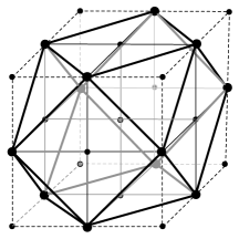
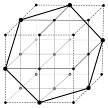
Figure 1: Genotopes for three loci: a cubeoctahedron and a hexagon.

We illustrate the concept of a genotope for the case of $n=3$ loci. Here $\mathcal{G}$ is any subset of the $27$ genotypes in $\{0,1,2\}^{3}$, and the genotope ${\rm conv}(G)$ is a convex polytope of dimension at most three. A basic invariant of such a polytope is the triple $(v,e,f)$ where $v$ is the number of vertices, $e$ is the number of edges and $f$ is the number of facets. Figure 1 shows three concrete examples:

• If ${\cal G}=\{0,1,2\}^{3}$ then the genotope $\,{\rm conv}(G)$ is the three-dimensional cube with side lengths two. It has $(v,e,f)=(8,12,6)$. The eight vertices correspond to the genotypes that are homozygous at all three sites.

• If the eight purely homozygous genotypes cannot occur in a population then ${\cal G}$ consists of the remaining $19$ genotypes. Now the genotope ${\rm conv}(G)$ is a cubeoctahedron, with $(v,e,f)=(12,24,14)$. Its twelve vertices correspond to genotypes with precisely two homozygous sites.

• If the alleles at all three sites must be distinct then

  $${\cal G}\,\,\,=\,\,\,\bigl{\{}(012),(021),(102),(120),(201),(210)\bigr{\}},$$

  and the dimension of the genotope drops to two. It is a regular hexagon with $(v,e,f)=(6,6,0)$.

The theory developed in [1] concerns gene interactions and the shapes of fitness landscapes. By definition, a fitness landscape is any function $\,w:\mathcal{G}\rightarrow\mathbb{R}$. In population genetics, $w(g)$ measures the expected number of offspring of an individual with genotype $g\in\mathcal{G}$. The regular triangulations of the genotope describe epistatic interactions among the genotypes. In the context of human genetics, it makes sense to replace the notion of fitness by penetrance values for a disease [14] or by expression levels of a gene [5]. A classification of two-dimensional genotopes and their triangulations from this perspective is presented in [11].

We cannot construct the human genotope at this time because the HapMap project is not complete. However, in Section 3 we explain how the existing preliminary HapMap data can already be used to reveal something about the human genotope. By restricting our attention to the ENCODE regions, and by taking advantage of linkage disequilibrium, we are able to compute biologically meaningful low-dimensional projections of the human genotope.

3 Human Variation Data

In this section we explain the data we used, how they were obtained, and how they were prepared. Our data consists of 269 genotypes over dbSNP loci in the two ENCODE regions ENr131 and ENm014 sampled by the HapMap project. These are the two regions listed in [12, Table 8]. In our study, we used the non-redundant version of the dataset which is available for download at

www.hapmap.org/genotypes/latest_ncbi_build34/ENCODE/

The data are grouped into four populations: Utah-European (CEU), Han-Chinese (CHB), Japanese (JPT) and Yoruba (YRI). The region ENm014 has 2315 SNPs, of which 1968 were sampled in all four populations. Only one of the SNPs was triallelic in the HapMap data, but many SNPs had incomplete data due to sequencing errors. In fact the number of SNPs in ENm014 successfully sequenced in all 269 individuals is 790, about a third of the total number of SNPs. It seems that a disproportionate number of loci in region ENm014 had missing data, evidently due to unusual sequencing problems in several individuals.

For simplicity we restricted our attention to the portion of SNP loci that had two or fewer observed alleles in the HapMap data, and which were successfully sampled in all 269 HapMap individuals. This implies that our projections of the human genotope are all representable as subpolytopes of a standard hypercube. After so restricting the set of loci, our data comprise 269 diploid genotypes, over 1154 loci from region ENr131 and 790 loci from region ENm014.

For each SNP locus, the lexicographically smaller nucleotide was used as the reference allele, and each of the observed 269 diploid genotypes was encoded as a numerical genotype in $\{0,1,2\}$. For example, for each SNP locus with nucleotide $A$ or $G$ we have $AA=0$, $GG=2$, and $AG=GA=1$. We thereby encoded the 269 genotypes as a $269\times 1154$ matrix over $\{0,1,2\}$ for region ENr131 and a $269\times 790$ matrix for region ENm014. The convex hull of the rows of one of our matrices gives a projection of a subpolytope of the human genotope.

As an illustration of our data, below is the $10\times 15$ upper left submatrix of the matrix for region ENr131. It encodes the first 15 out of the 1154 biallelic SNPs, which were sampled in our first 10 HapMap individuals in the CEU population:

$${\tt\left({\begin{tabular}[]{ccccccccccccccc}2&0&2&0&2&0&2&0&0&0&2&0&2&2&1\\ 2&0&2&0&2&0&2&0&1&0&2&1&1&1&0\\ 2&1&2&0&1&1&2&0&1&0&1&1&1&1&1\\ 2&0&2&0&2&0&2&1&0&0&2&2&0&0&0\\ 1&1&2&0&1&0&2&1&0&0&1&2&0&0&0\\ 1&0&2&0&2&0&2&0&0&0&2&1&1&1&0\\ 1&0&2&0&2&0&2&0&0&0&2&1&1&1&0\\ 1&0&2&0&2&0&2&1&0&0&2&2&0&0&0\\ 2&0&2&0&2&0&2&0&0&0&2&1&1&1&1\\ 2&0&2&0&2&0&2&0&0&0&2&1&1&1&1\\ \end{tabular}}\right)}$$

Already in the above submatrix we see likely linkage between the 5th and 6th columns, and also between the 12th, 13th, and 14th columns. Such covariance among SNPs will allow us to work with various projections of genotopes, which we discuss in the following sections. We also note that the individuals in rows 6 and 7 as well as those in rows 9 and 10 have identical sequences in this matrix. The eight distinct rows in this example are affinely independent, so this projection of the human genotope into $\mathbb{R}^{15}$ is a $7$-dimensional simplex.

All of our data, along with the Linux utility used to convert the HapMap data files into matrices can be downloaded at our supplementary website

bio.math.berkeley.edu/humangenotope/

The utility takes the four population files for a particular ENCODE region, downloaded from the above hapmap site, and it converts each file into the corresponding matrix over $\{0,1,2\}$, in both MAPLE and MATLAB format.

4 Projections Onto Principal Components

Principal Component Analysis (PCA) is a standard statistical technique for reducing the dimension of high-dimensional data. In our study, the data is a $k\times n$-matrix $X$ with entries in $\{0,1,2\}$. The genotope under consideration is the convex hull of the row vectors of the matrix $X$. Our mathematical problem consists of applying PCA to our data in a manner that is consistent with the affine geometry of convex polyhedra. For this reason, we augment the matrix $X$ to a $k\times(n+1)$-matrix $X^{\prime}$ by adding a column of $1$’s. In our situation, we have $n\geq k$, and PCA amounts to computing the singular value decomposition

$$X^{\prime}\quad=\quad U\cdot\Sigma\cdot V,$$

where $\Sigma$ is a real diagonal $k\times(n+1)$-matrix whose main diagonal entries satisfy $\sigma_{1}\geq\sigma_{2}\geq\cdots\geq\sigma_{k}\geq 0$. The columns of the $k\times k$-matrix $U$ are the left singular vectors of $X^{\prime}$; they form an optimal orthonormal basis for the column space of $X^{\prime}$. Likewise, the rows of the $(n+1)\times(n+1)$-matrix $V$ are the right singular vectors of $X^{\prime}$; they are an optimal orthonormal basis of the row space of $X^{\prime}$. Here optimality means that the matrix obtained from $U\cdot\Sigma\cdot V$ by setting $\,\sigma_{\ell+1}=\cdots=\sigma_{k}=0\,$ is closest (in the Euclidean norm) to $X^{\prime}$ among all $k\times(n+1)$-matrices of rank $\leq\ell$.

Consider any positive integer $\,\ell\leq k$. Let $\,(\Sigma\cdot V)_{\ell}\,$ denote the submatrix of $\,\Sigma\cdot V\,$ consisting of the first $\ell$ columns. We define the $\ell$-th PCA projection of the genotope represented by $X$ to be the convex hull in $\mathbb{R}^{\ell}$ of the row vectors of the matrix $(\Sigma\cdot V)_{\ell}$. This polytope can be regarded as the statistically most significant orthogonal projection into $\mathbb{R}^{\ell}$ of the given genotope in $\mathbb{R}^{n}$.

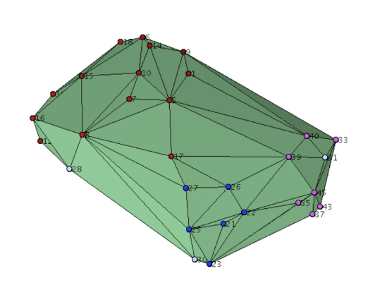
Figure 2: The 3-dimensional PCA projection of the ENr131 ENCODE genotope. The colors of the vertices represent the different populations: red=CEU, blue=CHB, cyan=JPT, pink=YRI.

The numerical computation of PCA projections is straightforward, equivalent to computing the SVD of the data matrix. Using MATLAB on a Pentium 4 PC, we can compute PCA projections of a HapMap ENCODE region in a matter of seconds. However, there are non-trivial numerical issues with these computations which makes them more difficult in our case. What we are seeking is the correct combinatorial structure of the genotopes and their projections. However, arbitrarily small round-off errors can change the combinatorics of a polytope. An example is the standard $3$-dimensional cube: if we slightly perturb one vertex, then at least one square face will be broken into two triangles.

To solve this round-off problem, we computed each PCA projection of our ENCODE genotopes using very high precision arithmetic. Whenever we observed a facet of a projected genotope nearly parallel to one of its neighboring facets, we merged the two facets together. This process gives the correct facets.

$\ell$	$\sigma_{\ell}$ (r131, m014)	ENr131   $f$-vector	ENm014   $f$-vector
$1$	$696,\,611$	$(\,2\,)$	$(\,2\,)$
$2$	$117,\,76$	$(\,11,\,11\,)$	( 10,  10 )
$3$	$91,\,64$	$(\,46,\,132,\,88\,)$	$(41,\,117,\,78\,)$
$4$	$69,\,52$	$(\,82,\,505,\,846,\,423\,)$	$(90,\,549,\,918,\,459\,)$
$5$	$67,\,41$	$(\,135,\,1567,\,4938,$	$(136,\,1582,\,4988,$
		$\,\,\,\,\,\,\,\,\,\,\,\,\,\,\,\,\,\,\,\,\,\,\,\,\,\,\,5840,\,2336\,)$	$\,\,\,\,\,\,\,\,\,\,\,\,\,\,\,\,\,\,\,\,\,\,\,\,\,\,\,5900,\,2360\,)$
$6$	$57,\,37$	$(\,179,\,3570,\,18699,\,$	$(\,182,\,3544,\,18370,$
		$\,\,\,\,\,\,\,\,\,\,\,39142,\,35751,\,11917\,)$	$\,\,\,\,\,\,\,\,\,\,\,38300,\,34938,\,11646\,)$

Table 1: Singular values and $f$-vectors of the $\ell$-th PCA projection of the ENCODE genotopes for regions ENr131 and ENm014, for $\ell=2,3,4,5,6$.

We computed the $\ell$-th PCA projection of the two ENCODE genotopes for $\ell$ up to $6$. For each projection we give the $f$-vector, which records the number of faces of each dimension. The results are shown in Table 1. We note that the first few principal components explain most of the variation in the data, and that the $f$-vectors of the $\ell$-th PCA projections are quite similar between the two regions. Figure 2 shows the 3-dimensional PCA projection of the ENr131 genotope. The $f$-vector is $(46,132,88)$ which means that the polytope has $46$ vertices, $132$ edges, and $88$ facets. Each vertex of the polytope is a projection of one of the $269$ genotypes in the four populations, which are indicated by colors.

We found that the projected genotopes give an excellent representation of the four different populations, in the sense that they correspond to four distinct regions on the polytope boundary. The only exception in Figure 2 is one of the Japanese genotypes that occurs among the Utah genotypes. While this may be a coincidence, it is noteworthy that only the identification of Japanese in the genotyping process was solely based on self-reporting.

5 Projections Onto Few SNPs

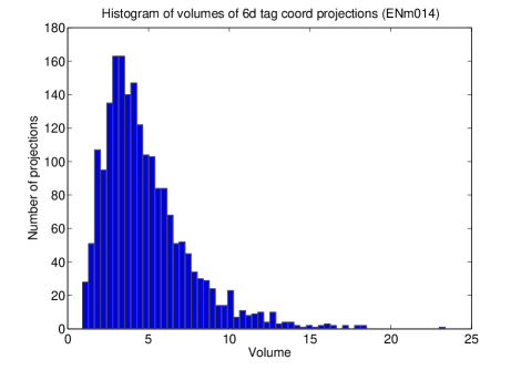
Figure 3: Volumes of projections of the ENm014 genotope onto tag SNPs.

In this section we discuss coordinate projections of the ENCODE genotopes. Such projections are relevant because of the commonplace practice of selecting tag SNPs for genetics studies. Such SNPs are subsets of the available SNPs that are, as much as possible, in pairwise linkage disequilibrium. Thus, despite the fact that $\ell$ tag SNPs capture less of the variation in the data than the $\ell$th PCA projection, they are useful in re-sequencing applications where it is desirable to sample as few SNPs as possible.

The polyhedral analog of restricting analysis to tag SNPs is the projection of the genotope onto the tag SNP coordinates. Each individual projection onto $\ell$ SNPs is easy to compute, provided $\ell$ is not too big. What makes the computation of all coordinate projections challenging is the combinatorial explosion in the number of $\ell$-element subsets of the $n$ SNPs. We did not attempt to exhaustively compute all of these projections. Instead we computed the projections of the two ENCODE genotopes onto tag SNPs selected for further study.

Using the software Hclust.R [16], we chose 35 tags out of the 790 SNPs for region ENm014, and 109 tags out of the 1154 SNPs for region ENr131. These rather small sets of tag SNPs still capture most of the variation in the data: for region ENm014, the sum of estimated variances of the original 790 columns is 108, and after projecting all columns onto the span of the 35 tag columns (and an added column of ones), the sum of the 790 estimated variances is 95. Similarly for region ENr131, the original sum of estimated variances is 288, and becomes 274 after projecting. Many of the SNPs not chosen as tags were monomorphic in the HapMap data, or had low observed minor allele frequencies. For example, in region ENm014 there were 206 monomorphic sites and 331 with low minor allele frequency. Hclust.R reported that 253 candidate SNPs were considered for region ENm014, and 726 candidate SNPs were considered for region ENr131. We then investigated random samples of coordinate projections of the ENCODE projections onto $\ell$ tag SNPs for $\ell=2,3,4,5,6$. This computation of tens of thousands of polytopes was accomplished by automating polyhedral software. The packages we used are polymake [9] and iB4e [7].

Our geometric analysis suggests a new test for identifying informative SNPs. For each coordinate projection, we compute the volume of the resulting projected genotope. Since points in a genotope correspond to allele frequency vectors which can be realized by populations over the genotypes, there is a natural probabilistic interpretation of such volumes of genotopes. The volume criterion seeks to identify the subset of $\ell$ SNPs which maximizes this polytope volume.

As an example of our coordinate projections data, Figure 3 shows the empirical distribution of the volumes of the $6d$ tag SNP projections of the ENm014 genotope. In our random sample of 2000 6d projections onto tag SNPs for region ENm014, the largest volume we observed was 23.36. The projection attaining this maximal volume is a genotope with 84 vertices and 377 facets, which is high compared to randomly chosen 6d projections onto tag SNPs. Moreover, this particular 6d projection explains almost half of the variation in our data matrix for region ENm014. Out of the random sample of 2000 6d tag SNP projections, only 13 produced a higher sum of variances of the projected columns. We take this as strong empirical support for our proposed volume criterion.

6 Archetypal Analysis

Archetypal analysis was introduced by Cutler and Breiman [4] as an alternative to PCA. Its aim is to find low-dimensional projections of the data points onto meaningful mixtures of the high-dimensional points. Our data points in this section are the rows of our data matrix $X$, i.e., the $k$ genotypes $x_{1},\ldots,x_{k}\in\{0,1,2\}^{n}$. They represent the individuals in the four populations.

Archetypal analysis finds archetypes that have the property that when each genotype is replaced by its nearest mixture of archetypes, the total least squares error is minimal. More precisely, if $\ell$ is the number of archetypes to be found (specified by the user), then the goal is to find archetypes $z_{1},\ldots,z_{\ell}$ together with $\alpha_{im}$ and $\beta_{mi}$ ($0\leq\alpha_{im},\beta_{mi}$ and $\sum_{m}\alpha_{im}=\sum_{i}\beta_{mi}=1$) such that

$$z_{m}\quad=\quad\sum_{j=1}^{k}\beta_{mj}x_{j},\qquad m=1,\ldots,\ell,$$

and

$$\sum_{i=1}^{k}||x_{i}-\sum_{m=1}^{\ell}\alpha_{im}z_{m}||^{2}$$

is minimized.

The benefit of archetypal analysis is that the archetypes have a useful and meaningful interpretation. For the data studied here, the archetypes are mixtures of genotypes. Thus the inferred archetypes can be interpreted as representative populations for the measured genotypes. No efficient algorithm is known that guarantees finding the $\ell$ optimal archetypes, but the alternating optimization procedure suggested in [4, §4.1] appears to perform well in practice.

In our view, computing archetypes from human variation data may be useful for designing population based genetic studies. In particular, the allele frequencies of the archetype populations suggest sampling strategies for controls in case-control studies, where it may be useful to sample a small number of groups of controls whose allele frequencies match the archetype populations.

We now explain our implementation of archetypal analysis. The function to be minimized is a large biquadratic polynomial, that is, a polynomial which is separately quadratic in two groups of unknowns. This biquadratic polynomial is the residual sum of squares (RSS) whose derivation is given in [4, §4]. Our problem is to minimize the residual sum of squares subject to non-negativity constraints. This optimization problem can have many local minima, and, in general, we cannot hope to find the global minima. The heuristic of alternating optimization for computing local minima works as follows. If we keep one of the two sets of variables fixed, then the objective function is just quadratic in the other set of unknowns and we can easily find the global minimum. We then fix those values and we allow the other set of unknowns to vary, solving again a quadratic optimization problem. Iterating this procedure leads to a local optimum [4, §5]. This process can be repeated with many different starting values to reach a local optimum that is eventually satisfactory.

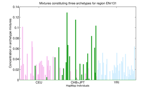
Figure 4: Thearchetypes for region ENr131 showing the population structure.

We implemented this alternating optimization algorithm in MATLAB, using the high-performance optimization package SeDuMi [17] to solve the arising quadratic optimization subproblems. As a heuristic to speed up computations, we first restricted our attention to tag SNPs and computed archetypes for these much smaller data sets. We then used the obtained archetypes as an initial guess for the archetypes in the full-dimensional data.

We computed sets of three archetypes for ENr131 and ENm014. The number $\ell=3$ is of particular interest in our study since we advocate that archetypes should be interpreted as representative populations, and the HapMap data is derived from three populations (CEU, JPT+CHB, and YRI).

Figure 4 depicts the three archetypes computed for region ENr131. By definition, each archetype can be expressed as a mixture $\sum\beta_{i}x_{i}$ where the $x_{i}$ are the genotypes of the 269 HapMap individuals, and all $\beta_{i}\geq 0$, with $\sum\beta_{i}=1$. For each archetype, we plot the 269 coefficients $\beta_{i}$ as 269 bars in the figure. We plotted all three archetypes on the same figure, using a different bar color for each archetype. We confirm that the three archetypes correspond to the three main geographic populations CEU, JPT+CHB, and YRI. Although there is some mixing between CEU and JPT+CHB in two of the archetypes, the third archetype is purely YRI and it is the only archetype containing YRI. This is consistent with the fact that YRI is an outgroup among the three populations.

7 Discussion

As the amount of human variation data continues to increase, it is becoming imperative to find representations of the data that are informative and convenient for analysis. The human genotope offers one such representation: a geometric description of the data that is useful for studying population structure and epistasis. In this paper, we have computed three low-dimensional projections of a subpolytope of the human genotope. The projections are all compatible with the geometric structure of the genotope, and are useful in different ways.

In terms of population structure, we believe that the results using archetypal analysis are particularly interesting, and we were surprised at the natural separation of the populations that emerged in the archetypes (Figure 4). In our computations we picked the number of archetypes to be $\ell=3$ based on information we had about the data. In general, it is an interesting problem to determine, in a statistically meaningful way, the “optimal” number of archetypes to use for an analysis. We believe that information theoretic measures, such as the Jensen-Shannon divergence, may be useful for this problem [10]. The principal component projections in Section 4 demonstrate that the genotope is a representation that is compatible with existing approaches to dimensionality reduction. In particular, we have shown that principal component projections can be applied to polytopes, and not just points. Our results in Figure 2 offer a geometric analog of Cavalli-Sforza’s gene-based population analyses [3].

We conclude by reiterating that our results are an initial first step towards the construction of the human genotope. Next steps include the extension to more SNPs, association of phenotype data with the genotypes so that epistasis can be studied, and an analysis of how the genotope changes over time.

References

- [1] N. Beerenwinkel, L. Pachter and B. Sturmfels, Epistasis and shapes of fitness landscapes, to appear in Statistica Sinica, ArXiv:q-bio.PE/0603034.
- [2] N. Beerenwinkel, L. Pachter, B. Sturmfels, S. Elena, R. Lenski, Analysis of epistatic interactions and fitness landscapes using a new geometric approach, submitted.
- [3] L.L. Cavalli-Sforza, P. Menozzi and A. Piazza, The History and Geography of Human Genes, Princeton University Press (1994).
- [4] A. Cutler and L. Breiman, Archetypal analysis, Technometrics 36 (1994) 338–347.
- [5] E.J. Chesler, L. Lu, S. Shou, Y. Qu, J. Gu, J. Wang, H.C. Hsu, J. D. Mountz, N.E. Baldwin, M. A. Langston et al., Complex trait analysis of gene expression uncovers polygenic and pleiotropic networks that modulate nervous system function, Nature Genetics, 37 (2005) 233–242.
- [6] F.B. Christiansen, Population Genetics of Multiple Loci, Wiley (2000).
- [7] C. Dewey, P. Huggins, K. Woods, B. Sturmfels and L. Pachter, Parametric alignment of Drosophila genomes, PLoS Computational Biology 2(6) (2006) p e73.
- [8] The ENCODE project consortium, The ENCODE (ENCylopedia Of DNA Elements) Project, Science 306(5696) (2004) 636–640.
- [9] E. Gawrilow, M. Joswig, Geometric reasoning with polymake, arXiv:math/0507273
- [10] I. Grosse, P. Bernaola-Galván, P. Carpena, R. Román-Roldán, J. Oliver and H.E. Stanley, Analysis of symbolic sequences using the Jensen-Shannon divergence, Physical Review E 65(041904-1) (2002) 1063–1065.
- [11] I. Hallgrímsdóttir, D. Yuster: A complete classification of two-locus disease models, submitted.
- [12] The International HapMap Consortium, A haplotype map of the human genome, Nature 437(7063) (2005) 1299–1320.
- [13] G. Kimmel and R. Shamir, A block-free hidden Markov model for genotypes and its application to disease association, Journal of Computational Biology 12(10) (2005) 1243–1260.
- [14] J. Ott, Analysis of Human Genetic Linkage (3rd edition), Johns Hopkins University Press (1999).
- [15] A.L. Price, N.J. Patterson, R.M. Plenge, M.E. Weinblatt, N.A. Shadlick, D. Reich, Principal components analysis corrects for stratification in genome-wide association studies, Nature Genetics 38 (2006) 904–909.
- [16] A. Rinaldo, S.A. Bacanu, B. Devlin, V. Sonpar, L. Wasserman, K. Roeder, Characterization of multilocus linkage disequilibrium, Genetic Eipdemiology 28(3) (2005) 193–206.
- [17] J.F. Sturm, Using SeDuMi, a Matlab toolbox for optimization over symmetric cones, Optimization Methods and Software 11–12 (1999) 625–653.