Evolution Equation of Phenotype Distribution: General Formulation and Application to Error Catastrophe

Abstract

An equation describing the evolution of phenotypic distribution is derived using methods developed in statistical physics. The equation is solved by using the singular perturbation method, and assuming that the number of bases in the genetic sequence is large. Applying the equation to the mutation-selection model by Eigen provides the critical mutation rate for the error catastrophe. Phenotypic fluctuation of clones (individuals sharing the same gene) is introduced into this evolution equation. With this formalism, it is found that the critical mutation rate is sometimes increased by the phenotypic fluctuations, i.e., noise can enhance robustness of a fitted state to mutation. Our formalism is systematic and general, while approximations to derive more tractable evolution equations are also discussed.

I Introduction

For decades, quantitative studies of evolution in laboratories have used bacteria and other microorganismsLenski ; Lenski-Rose ; Kishony . Changes in phenotypes, such as enzyme activity and gene expressions introduced by mutations in genes, are measured along with the changes in their population distribution in phenotypes Bactreia-many-generations ; Dekel-Alon ; Kashiwagi-Noumachi ; Ito . Following such experimental advances, it is important to analyze the evolution equation of population distribution of concerned genotypes and phenotypes.

In general, fitness for reproduction is given by a phenotype, not directly by a genetic sequence. Here, we consider evolution in a fixed environment, so that the fitness is given as a fixed function of the phenotype. A phenotype is determined by mapping a genetic sequence. This phenotype is typically represented by a continuous (scalar) variable, such as enzyme activity, protein abundances, and body size. For studying the evolution of a phenotype, it is essential to establish a description of the distribution function for a continuous phenotypic variable, where the fitness for survival, given as a function of such a continuous variable, determines population distribution changes over generations.

However, since a gene is originally encoded on a base sequence (such as AGCTGCTT in DNA), it is represented by a symbol sequence of a large number of discrete elements. Mutation in a sequence is not originally represented by a continuous change. Since the fitness is given as a function of phenotype, we need to map base sequences of a large number of elements onto a continuous phenotypic variable $x$, where the fitness is represented as a function of $x$, instead of the base sequence itself. A theoretical technique and careful analysis are needed to project a discrete symbol sequence onto a continuous variable.

Mutation in a nucleotide sequence is random, and is represented by a stochastic process. Thus, a method of deriving a diffusion equation from a random walk is often applied. However, the selection process depends on the phenotype. If a phenotype is given as a function of a sequence, the fitness is represented by a continuous variable mapped from a base sequence. Since the population changes through the selection of fitness, the distribution of the phenotype changes accordingly. If the mapping to the phenotype variable is represented properly, the evolutionary process will be described by the dynamics of the distribution of the variable, akin to a Fokker-Planck equation.

In fact, there have been several approaches to representing the gene with a continuous variable footnote . KimuraKimura2 developed the population distribution of a continuous fitness. Also, for certain conditions, a Fokker-Planck type equation has been analyzed by LevineLevine . Generalizing these studies provides a systematic derivation of an equation describing the evolution of the distribution of the phenotypic variable. We adopt selection-mutation models describing the molecular biological evolution discussed by EigenEigen , Kauffmankauffmann-book , and others, and take a continuum limit assuming that the number of bases $N$ in the genetic sequence is large, and derive the evolution equation systematically in terms of the expansion of $1/N$.

In particular, we refer to Eigen’s equationEigen , originally introduced for the evolution of RNA, where the fitness is given as a function of a sequence. Mutation into a sequence is formulated by a master equation, which is transformed to a diffusion-like equation. With this representation, population dynamics over a large number of species is reduced to one simple integro-differential equation with one variable. Although the equation obtained is a non-linear equation for the distribution, we can adopt techniques developed in the analysis of the (linear) Fokker-Planck equation, such as the eigenfunction expansion and perturbation methods.

So far, we have assumed a fixed, unique mapping from a genotype to a phenotype. However, there are phenotypic fluctuations in individuals sharing the same genotype, which has recently been measured quantitatively as a stochastic gene expression Koshland ; Elowitz ; Kaern-Collins ; Collins ; Furusawa ; Ueda ; noise-review . Relevance of such fluctuations to evolution has also been discussedSatoPNAS ; kaneko-book ; KKFurusawaJTB ; Ancel . In this case, mapping from a gene gives the average of the phenotype, but phenotype of each individual fluctuates around the average. In the second part of the present paper, we introduce this isogenic phenotypic fluctuation into our evolution equation. Indeed, our framework of Fokker-Planck type equations is fitted to include such fluctuations, so that one can discuss the effect of isogenic phenotypic fluctuations on the evolution.

The outline of the present paper is as follows: We first establish a sequence model in section (II). For deriving the evolution equation from the sequence model, we postulate the assumption that the transition probability of phenotype values is uniquely determined by the original phenotype value. The assumption may appear too demanding at a first sight, but we show that it is not unnatural from the viewpoint of evolutionary biology. In fact, most models studied so far satisfy this postulate. With this assumption, we derive a Fokker-Planck type equation of phenotypic distribution using the Kramers-Moyal expansion method from statistical physicsvanKampen ; KuboMatsuoKitahara . We discuss the validity of this expansion method to derive the equation, also from a biological point of view.

As an example of the application of our formulation, we study the Eigen’s model in section (III), and estimate the critical mutation rates at which error catastrophe occurs, using a singular perturbation method. In section (V), we discuss the range of the applicability of our method and discuss possible extensions to it.

Following the formulation and application of the Fokker-Planck type equations for evolution, we study the effect of isogenic phenotypic fluctuations. While fluctuation in the mapping from a genotype to phenotype modifies the fitness function in the equation, our formulation itself is applicable. We will also discuss how this fluctuation changes the conditions for the error catastrophe, by adopting Eigen’s model.

For concluding the paper, we discuss generality of our formulation, and the relevance of isogenic phenotypic fluctuation to evolution.

II Derivation of evolution equation

We consider a population of individuals having a haploid genotype, which is encoded on a sequence consisting of $N$ sites (consider, for example, DNA or RNA). The gene is represented by this symbol sequence, which is assigned from a set of numbers, such as $\{-1,1\}$. This set of numbers is denoted by $S$. By denoting the state value of the $i$th site by $s_{i}$ ($\in S$), the configuration of the sequence is represented by the ordered set $s=\{s_{1},...,s_{N}\}$.

We assume that a scalar phenotype variable $x$ is assigned for each sequence $s$. This mapping from sequence to phenotype is given as function $x(s)$. Examples of the phenotype include the activity of some enzyme (protein), infection rate of bacteria virus, and replication rate of RNA. In general, the function $x(s)$ is a degenerate function, i.e., many different sequences are mapped onto the same phenotypic value $x$.

Each sequence is reproduced with rate $A$, which is assumed to depend only on the phenotypic value $x$, as $A(x)$; this assumption may be justified by choosing the phenotypic value $x$ to relate to the replication. For example, if a protein concerns with the metabolism of a replicating cell, its activity may affect the replication rate of the cell and of the protein itself.

In the replication of the sequence, mutation generally occurs; for simplicity, we consider only the substitution of $s(i)$. With a given constant mutation rate $\mu$ over all sites in the sequence, the state $s^{\prime}_{i}$ of the daughter sequence is changed from $s_{i}$ of the mother sequence, where the value $s^{\prime}_{i}$ is assigned from the members of the set $S$ with an equal probability. We call this type of mutation symmetric mutation Baake2 . The mutation is represented by the transition probability $Q(s\rightarrow s^{\prime})$, from the mother $s$ to the daughter sequence $s^{\prime}$. The probability $Q$ is uniquely determined from the sequence $s$, the mutation rate $\mu$, and the number of members of $S$. The setup so far is essentially the same as adopted by Eigen et al.Eigen , where the fitness is given as a function of the RNA sequence or DNA sequence of virus.

Now, we assume that the transition probability depends only on the phenotypic value $x$, i.e., the function $Q$ can be written in terms of a probability function $W$, which depends only on $x$, $W(x\rightarrow x^{\prime})$, as

$$\sum_{s^{\prime}\in\{s^{\prime}|x^{\prime}=x(s^{\prime})\}}Q(s\rightarrow s^{\prime})=W(x(s)\rightarrow x^{\prime}).$$ (1)

This assumption may appear too demanding. However, most models of sequence evolution somehow adopt this assumption. For example, in Eigen’s model, fitness is given as a function of the Hamming distance from a given optimal sequence. By assigning a phenotype $x$ as the Hamming distance, the above condition is satisfied (this will be discussed later). In Kauffman’s NK model, if we set $N\gg 1$, $K\gg 1$, and $K/N\ll 1$, this assumption is also satisfied (see Appendix A). For the RNA secondary structure modelWaterman , this assumption seems to hold approximately, from statistical estimates through numerical simulations. Some simulations on a cell model with chemical reaction networksFurusawa ; Furusawa-KK also support the assumption. In fact, a similar assumption has been made in evolution theory with a gene substitution processGillespie ; Orr .

The validity of this assumption in experiments has to be confirmed. Consider a selection experiment to enhance some function through mutation, such as the evolution of a certain protein to enhance its activityIto . In this case, the assumption means that the activity distribution over the mutant proteins is statistically similar as long as they have the same activity, even though their mother protein sequences are different.

With the above setup, we consider the population of these sequences and their dynamics, allowing for overlap between generations, by taking a continuous-time modelBaake2 . We do not consider the death rate of the sequence explicitly since its consideration introduces only an additional term, as will be shown later. The time-evolution equation of the probability distribution $\hat{P}(s,t)$ of the sequence $s$ is given by:

$$\frac{\partial\hat{P}(s,t)}{\partial t}=-\bar{A}(t)\hat{P}(s,t)+\sum_{s^{\prime}}A(x(s^{\prime}))Q(s^{\prime}\rightarrow s)\hat{P}(s^{\prime},t),$$ (2)

as specified by EigenEigen . Here the quantity $\bar{A}(t)$ is the average fitness of the population at time $t$, defined by $\bar{A}(t)=\sum_{s}A(x(s))\hat{P}(s,t)$ and $Q$ is the transition probability satisfying $\sum_{s}Q(s^{\prime}\rightarrow s)=1$ for any $s^{\prime}$.

According to the assumption (1), eq. (2) is transformed into the equation for $P(x,t)$, which is the probability distribution of the sequences having the phenotypic value $x$, defined by $P(x,t)=\sum_{s\in\{s|x=x(s)\}}\hat{P}(s,t)$. The equation is given by

$$\frac{\partial P(x,t)}{\partial t}=-\bar{A}(t)P(x,t)+\sum_{x^{\prime}}A(x^{\prime})W(x^{\prime}\rightarrow x)P(x^{\prime},t),$$ (3)

where the function $W$ satisfies

$$\sum_{x}W(x^{\prime}\rightarrow x)=1\qquad\mbox{for any $x^{\prime}$,}$$ (4)

as shown.

Since $N$ is sufficiently large, the variable $x$ is regarded as a continuous variable. By using the Kramers-Moyal expansionvanKampen ; KuboMatsuoKitahara ; Haken , with the help of property (4), we obtain:

$$\frac{\partial P(x,t)}{\partial t}=(A(x)-\bar{A}(t))P(x,t)+\sum_{n=1}^{\infty}\frac{(-1)^{n}}{n!}\frac{\partial{}^{n}}{\partial x^{n}}m_{n}(x)A(x)P(x,t),$$ (5)

where $m_{n}(x)$ is the $n$th moment about the value $x$, defined by $m_{n}(x)=\int(x^{\prime}-x)^{n}W(x\rightarrow x^{\prime})dx^{\prime}$.

Let us discuss the conditions for the convergence of expansion (5), without mathematical rigor. For convergence, it is natural to assume that the function $W(x^{\prime}\rightarrow x)$ decays sufficiently fast as $x$ gets far from $x^{\prime}$, by the definition of the moment.

Here, the transition $W(x^{\prime}\rightarrow x)$ is a result of $n$ point mutants of the original sequence $s^{\prime}$ for $n=0,1,2,...,N$. Accordingly, we introduce a set of quantities, $w_{n}(x(s^{\prime})\rightarrow x)$, as the fitness distribution of $n$ point mutants of the original sequence $s^{\prime}$ (Naturally, $w_{0}(x(s^{\prime})\rightarrow x)=\delta(x(s^{\prime})-x)$, which does not contribute to the $n$th moment $m_{n}$ ($n\geq 1$)). Next, we introduce the probability $p_{n}$ that a daughter sequence is an $n$ point mutant $(n=0,1,2,...,N)$ from her mother sequence, which are determined only by the mutation rate $\mu$ and the sequence length $N$. Indeed, ${p_{n}}^{\prime}s$ form a binomial distribution, characterized by $\mu$ and $N$.

In terms of the quantities $w_{n}$ and $p_{n}$, we are able to write down the transition probability $W$ as

$$W(x(s^{\prime})\rightarrow x)=\sum_{n=0}^{N}p_{n}w_{n}(x(s^{\prime})\rightarrow x).$$ (6)

Now, we discuss if $W(x(s^{\prime})\rightarrow x)$ decays sufficiently fast with $|x(s^{\prime})-x|$. First, we note that the width of the domain, in which $w_{n}(x(s^{\prime})\rightarrow x)$ is not close to zero, increases with $n$ since $n$-point mutants involve increasing number of changes in the phenotype with larger values of $n$. Then, to satisfy the condition for $W(x(s^{\prime})\rightarrow x)$, at least the single-point-mutant transition $w_{1}(x(s^{\prime})\rightarrow x)$ has to decay sufficiently fast with $|x(s^{\prime})-x|$. In other words, the phenotypic value of a single-point mutant $s$ of the mother sequence $s^{\prime}$ must not vary much from that of the original sequence, i.e., $|x(s^{\prime})-x(s)|$ should not be large (“continuity condition”).

In general, the domain $|x-x(s^{\prime})|$, in which $w_{n}(x(s^{\prime})\rightarrow x)\neq 0$, increases with $n$. On the other hand, the term $p_{n}$ decreases with $n$ and with the power of $\mu^{n}$. Hence, as long as the mutation rate is not large, the contribution of $w_{n}$ to $W$ is expected to decay with $n$. Thus, if the continuity condition with regards to a single-point mutant and a sufficiently low mutation rate are satisfied, the requirement on $W(x(s^{\prime})\rightarrow x)$ should be fulfilled. Hence, the convergence of the expansion is expected.

Following the argument, we further restrict our study to the case with a small mutation rate $\mu$ such that $\mu N\ll 1$ holds. The transition probability $W$ in eq. (6) is written as

$$W(x(s^{\prime})\rightarrow x)\simeq(1-\mu N)\delta(x(s^{\prime})-x)+\mu Nw_{1}(x(s^{\prime})\rightarrow x),$$ (7)

where we have used the property that ${p_{n}}^{\prime}s$ form the binomial distribution characterized by $\mu$ and $N$. Introducing a new parameter, $\gamma$ ($\gamma=\mu N$), that gives the average of the number of changed sites at a single-point mutant, and using the transition probability (7), we obtain

$$\frac{\partial P(x,t)}{\partial t}=(A(x)-\bar{A}(t))P(x,t)+\gamma\sum_{n=1}^{\infty}\frac{(-1)^{n}}{n!}\frac{\partial{}^{n}}{\partial x^{n}}m_{n}^{(1)}(x)A(x)P(x,t),$$ (8)

where $m_{n}^{(1)}(x)$ is the $n$th moment of $w_{1}(x\rightarrow x^{\prime})$, i.e., $m_{n}^{(1)}(x)=\int(x^{\prime}-x)^{n}w_{1}(x\rightarrow x^{\prime})dx^{\prime}$.

When we stop the expansion at the second order, as is often adopted in statistical physics, we obtain

$$\frac{\partial P(x,t)}{\partial t}=(A(x)-\bar{A}(t))P(x,t)+\gamma\frac{\partial{}}{\partial x}\left[-m_{1}^{(1)}(x)+\frac{1}{2}\frac{\partial{}}{\partial x}m_{2}^{(1)}(x)\right]A(x)P(x,t).$$ (9)

Eqs. (8) and (9) are basic equations for the evolution of distribution function. Eq. (9) is an approximation. However, it is often more tractable, with the help of techniques developed for solving the Fokker-Planck equation ( see Appendix B and PhysicalBiology ), while there is no established standard method for solving eq. (8).

At the boundary condition we naturally impose that there are no probability flux, which is given by

$$\left.\sum_{n=1}^{\infty}\frac{(-1)^{n}}{n!}\frac{\partial{}^{(n-1)}}{\partial x^{(n-1)}}m_{n}^{(1)}(x)A(x)P(x,t)\right|_{x=x_{1},x_{2}}=0,$$ (10)

in the case of (8) and

$$\left.\left[-m_{1}^{(1)}(x)+\frac{1}{2}\frac{\partial{}}{\partial x}m_{2}^{(1)}(x)\right]A(x)P(x,t)\right|_{x=x_{1},x_{2}}=0$$ (11)

in the case of (9), where $x_{1}$ and $x_{2}$ are the values of the left and right boundaries, respectively.

Next, as an example of the application of our formula, we derive the evolution equation for Eigen’s model, and estimate the error threshold, with the help of a singular perturbation theory. Through this application, we can see the validity of eq. (9) as an approximation of eq. (8).

Two additional remarks: First, introduction of the death of individuals is rather straightforward. By including the death rate $D(x)$ into the evolution equation, the first term in eq. (8) (or eq. (9)) is replaced by $\left[(A(x)-D(x))-(\bar{A}(t)-\bar{D}(t))\right]P(x,t)$, where $\bar{D}(t)\equiv\int D(x)P(x,t)dx$. Second, instead of deriving each term in eq. (9) from microscopic models, it may be possible to adopt it as a phenomenological equation, with parameters (or functions) to be determined heuristically from experiments.

III Application of error threshold in Eigen model

In the Eigen modelEigen , the set $S$ of the site state values is given by $\{-1,1\}$, and the fitness (replication rate) of the sequence is given as a function of its Hamming distance from the target sequence $\{1,...,1\}$, i.e., the fitness of an individual sequence is given as a function of the number $n$ of the sites of the sequence having value $1$. Hence it is appropriate to define a phenotypic value $x$ in the Eigen model as a monotonic function of the number $n$; we determine it as $x=\frac{2n-N}{N}$, in the range $[-1,1]$. Accordingly, the replication rate $A$ of the sequence can be written as a function of $x$, i.e., $A(x)$; it is natural to postulate that $A$ is a non-negative and bounded function over the whole domain. If the sequence length $N$ is sufficiently large, the phenotypic variable $x$ can be regarded as a continuous variable, since the step size of $x$ ($\Delta x=\frac{2}{N}$) approaches 0 as $N$ goes to infinity.

In order to derive the evolution equation of form (8) corresponding to the Eigen model, we only need to know the function $w_{1}$ in that model. (Recall that in our formulation the mutation rate $\mu$ is assumed to be so small that only a single-point mutation is considered.) Due to the assumption of the symmetric mutation, this distribution function is obtained as $w_{1}(x\rightarrow x-\Delta x)=\frac{1+x}{2}$, $w_{1}(x\rightarrow x+\Delta x)=\frac{1-x}{2}$, and $w_{1}(x\rightarrow x^{\prime})=0$ for any other $x^{\prime}$. Accordingly, the $n$th moment is given by $m_{n}^{(1)}(x)=\frac{1+x}{2}(-\Delta x)^{n}+\frac{1-x}{2}(\Delta x)^{n}$. Now, we obtain

$$\frac{\partial P(x,t)}{\partial t}=(A(x)-\bar{A}(t))P(x,t)+\gamma\sum_{n=1}^{\infty}\frac{1}{n!}\frac{\partial{}^{n}}{\partial x^{n}}\left[\frac{1+x}{2}\left(\frac{2}{N}\right)^{n}+\frac{1-x}{2}\left(-\frac{2}{N}\right)^{n}\right]A(x)P(x,t)$$ (12)

where $\gamma=N\mu$, the mutation rate per sequence. When we ignore the moment terms higher than the second order, we have

$$\frac{\partial P(x,t)}{\partial t}=(A(x)-\bar{A}(t))P(x,t)+\frac{2\gamma}{N}\frac{\partial}{\partial x}\left[x+\frac{1}{N}\frac{\partial}{\partial x}\right]A(x)P(x,t).$$ (13)

In fact, if we focus on a change near $x\sim 0$ ( to be specific $x\sim O(1/\sqrt{N})$), the truncation of the expansion up to the second order is validated (Or equivalently, if we define $x^{\prime}=(2n-N)/\sqrt{N}$ instead of $(2n-N)/N$, and expand eq.(3) by $1/\sqrt{N}$ instead of $1/N$, terms higher than the second order are negligible, as is also discussed in Levine . However, in this case, the validity is restricted to $x^{\prime}\sim O(1)$ (i.e., $(n-N/2)\sim O(1)$), which means $x\sim O(1/\sqrt{N})$ in the original variable).

Now, we solve the eq. (13) with a standard singular perturbation method (see Appendix B), and then return to eq. (12). According to the analysis in Appendix B, the stationary solution of the equation of form (13) is given by the eigenfunction corresponding to the largest eigenvalue of the linear operator $L$ defined by $L=A(x)+2\gamma\varepsilon\frac{\partial}{\partial x}\left[x+\varepsilon\frac{\partial}{\partial x}\right]A(x)$ with $\varepsilon=\frac{1}{N}$. Now we consider the eigenvalue problem

$$A(x)P(x)+2\gamma\varepsilon\frac{\partial}{\partial x}\left[x+\varepsilon\frac{\partial}{\partial x}\right]A(x)P(x)=\lambda P(x),$$ (14)

where $P(x)\geq 0$, with $\lambda$ to be determined.

Since $\varepsilon$ is very small (because $N$ is sufficiently large), a singular perturbation method, the WKB approximationMorse-book , is applied. Let us put

$$P(x)=e^{\frac{1}{\varepsilon}\int_{x0}^{x}R(\varepsilon,x^{\prime})dx^{\prime}},$$ (15)

where $x_{0}$ is some constant and $R$ is a function of $\varepsilon$ and $x$, which is expanded with respect to $\varepsilon$ as

$$R(\varepsilon,x)=R_{0}(x)+\varepsilon R_{1}(x)+\varepsilon^{2}R_{2}(x)+...$$ (16)

Retaining only the zeroth order terms in $\varepsilon$ in eq. (14), we get

$$A(x)+2\gamma\left[xR_{0}(x)+R_{0}^{2}(x)\right]A(x)=\lambda,$$ (17)

which is formally solved for $R_{0}$ as $R_{0}^{(\pm)}(x)=\frac{-x\pm\sqrt{g(x)}}{2}$ where $g(x)=x^{2}+\frac{2}{\gamma}(\frac{\lambda}{A(x)}-1)$. Hence the general solution of eq. (14) up to the zeroth order in $\varepsilon$ is given by $P(x)=\alpha e^{\frac{1}{\varepsilon}\int_{x_{0}}^{x}R_{0}^{(+)}(x^{\prime})dx^{\prime}}+\beta e^{\frac{1}{\varepsilon}\int_{x_{0}}^{x}R_{0}^{(-)}(x^{\prime})dx^{\prime}}$ with $\alpha$ and $\beta$ constants to be determined.

Now, recall the boundary conditions (11); $P$ has to take the two branches in $R_{0}$ as $P(x)=\alpha e^{\frac{1}{\varepsilon}\int_{x_{b}}^{x}R_{0}^{(+)}(x^{\prime})dx^{\prime}}$ for $x<x_{b}$ and $P(x)=\beta e^{\frac{1}{\varepsilon}\int_{x_{b}}^{x}R_{0}^{(-)}(x^{\prime})dx^{\prime}}$ for $x>x_{b}$, where $x_{b}$ is defined as the value at which $g(x)$ has the minimum value. Next, from the continuity of $P$ at $x_{b}$, $\alpha=\beta$ follows, while from the continuity of $\frac{\partial P}{\partial x}$ at $x_{b}$, the function $g$ has to vanish at $x=x_{b}$. This requirement $g(x_{b})=0$ determines the value of the unknown parameter $\lambda$ as

$$\lambda=A(x_{b})(1-\frac{\gamma}{2}{x_{b}}^{2}).$$ (18)

From function $P$, we find that $P$ has its peak at the point $x=x_{p}$, where $R_{0}(x)$ vanishes, i.e., at $A(x_{p})=\lambda$. Then, $P(x)$ approaches $\delta(x-x_{p})$ in the limit $\varepsilon\rightarrow+0$. These results are consistent with the requirement that the mean replication rate in the steady state be equal to the largest eigenvalue of the system (see Appendix B).

The stationary solution of eq.(12) is obtained by following the same procedure of singular perturbation. Consider the eigenvalue problem

$$A(x)P(x)+\gamma\sum_{n=1}^{\infty}\frac{1}{n!}\frac{\partial{}^{n}}{\partial x^{n}}\left[\frac{1+x}{2}\left(2\varepsilon\right)^{n}+\frac{1-x}{2}\left(-2\varepsilon\right)^{n}\right]A(x)P(x)=\lambda P(x).$$ (19)

By putting $P(x)=e^{\frac{1}{\varepsilon}\int_{x0}^{x}R_{0}(x^{\prime})dx^{\prime}}$ and taking only the zeroth order terms in $\varepsilon$, we obtain

$$A(x)+\gamma\left[\frac{1+x}{2}\left(e^{2R_{0}(x)}-1\right)+\frac{1-x}{2}\left(e^{-2R_{0}(x)}-1\right)\right]A(x)=\lambda,$$

which gives

$$R_{0}^{(\pm)}(x)=\frac{1}{2}\log\frac{1+\frac{1}{\gamma}(\frac{\lambda}{A(x)}-1)\pm\sqrt{\hat{g}(x)}}{1+x}$$

with $\hat{g}(x)=(1+\frac{1}{\gamma}(\frac{\lambda}{A(x)}-1))^{2}-(1-x^{2})$.

By defining again the value $x=x_{b}$ at which $\hat{g}(x)$ takes the minimum, $P$ is represented as $P(x)=\alpha e^{\frac{1}{\varepsilon}\int_{x_{b}}^{x}R_{0}^{(+)}(x^{\prime})dx^{\prime}}$ for $x<x_{b}$ and $P(x)=\beta e^{\frac{1}{\varepsilon}\int_{x_{b}}^{x}R_{0}^{(-)}(x^{\prime})dx^{\prime}}$ for $x>x_{b}$. The continuity of $\frac{\partial P}{\partial x}$ at $x=x_{b}$ requires $\hat{g}(x_{b})=0$, which determines the value of $\lambda$ as

$$\lambda=A(x_{b})\left[1-\gamma\left(1-\sqrt{1-{x_{b}}^{2}}\right)\right].$$ (20)

Again, $P(x)=\delta(x-x_{p})$, in the limit $\varepsilon\rightarrow+0$, with $x_{p}$ given by the condition $A(x_{p})=\lambda$. When $|x_{b}|\ll 1$, the form (20) approaches eq. (18) asymptotically. This implies that the time evolution equation (8), if restricted to $|x|\ll 1$, is accurately approximated by eq.(9) that keeps the terms only up to the second moment.

Let us estimate the threshold mutation rate for error catastrophe. This error threshold is defined as the critical mutation rate $\gamma^{*}$ at which the peak position $x_{p}$ of the stationary distribution drops from $x_{p}\neq 0$ to $x_{p}=0$, with an increase of $\gamma$. We use the following procedure to obtain the critical value $\gamma^{*}$.

First consider an evaluation function whose form corresponds to that of eigenvalue (20) as

$$f(x)=A(x)\left[1-\gamma\left(1-\sqrt{1-{x}^{2}}\right)\right],$$ (21)

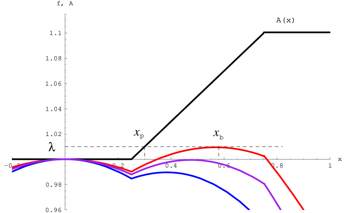
Figure 1: Examples of profiles of the evaluation function $f$ for three values of $\gamma$. The red, purple, and blue curves give the profiles of $f$ for $\gamma=0.31$, $\gamma=0.386$, and $\gamma=0.49$, respectively, where $f$ is defined by $f(x)=A(x)(1-\gamma(1-\sqrt{1-x^{2}}))$ and $A$ is given by $A(x)=1+0.2(x-0.25)\Theta(x-0.25)\Theta(0.75-x)+0.1\Theta(x-0.75)$; the profile of $A$ is indicated by the black curve. This illustrates determination of $x_{b}$ and $x_{p}$; $x_{b}$ is given by the position where $f$ takes a maximum, while $x_{p}$ is given as the position where the line $y=f(x_{b})$ crosses the curve of $A$. For $\gamma<0.386$, $f(x)$ has a maximum value at $x=x_{b}$, and thus the critical mutation rate for the error threshold is estimated to be $\gamma^{*}=0.386$.

and find the position at which the function $f(x)$ takes the maximum value. This procedure is equivalent to obtaining $x_{b}$ in the above analysis, since the relation $f(x)=\lambda-\frac{\gamma^{2}A^{2}(x)}{\lambda-A(x)\left(1-\gamma\left(1+\sqrt{1-x^{2}}\right)\right)}\hat{g}(x)$ and the requirement on $x_{b}$ that $\hat{g}(x_{b})=0$ and $\left.\frac{d\hat{g}(x)}{dx}\right|_{x=x_{b}}=0$ lead to $\left.\frac{df(x)}{dx}\right|_{x=x_{b}}=0$. Obviously, $x_{b}$ is given as a function of $\gamma$, thus, we denote it by $x_{b}(\gamma)$. The position $x_{b}$ determines the position $x_{p}$ of the stationary distribution through the relation $A(x_{p})=\lambda=f(x_{b})$ as in the above analysis. If $A$ has flat parts around $x=0$ and higher parts in the region ($x>0$), $x_{p}(\gamma)$ discontinuously changes from $x_{p}\neq 0$ to $x_{p}=0$ at some critical mutation rate $\gamma^{*}$, when $\gamma$ increases from zero. A schematic illustration of this transition is given in Fig.(1).

As a simple example of this estimate of error threshold, let us consider the case

$$A(x)=1+A_{0}\Theta(x-x_{0}),$$ (22)

with $A_{0}>0$ and $0<x_{0}<1$, and $\Theta$ as the Heaviside step function, defined as $\Theta(x)=0$ for $x<0$ and $\Theta(x)=1$ for $x\geq 0$. According to the procedure given above, the critical mutation rate is straightforwardly obtained as $\gamma^{*}=\frac{A_{0}}{(1+A_{0})\left(1-\sqrt{1-{x_{0}}^{2}}\right)}$, for $\gamma<\gamma^{*}$, $x_{p}=x_{0}$ and for $\gamma>\gamma^{*}$, $x_{p}=0$.

Remark

An exact transformation from the sequence model (Eigen modelEigen ) into a class of Ising modelsLeuthausser ; Baake has recently been reported, such that the sequence model is treated analytically with methods developed in statistical physics. Rigorous estimation of the error threshold for various fitness landscapesBaake2 ; Taiwan and relaxation times of species distribution have been obtainedTaiwan2 . In fact, our estimate (above) agrees with that given by their analysis.

Their method is indeed powerful when a microscopic model is prescribed in correspondence with a spin model. However, even if such microscopic model is not given, our formulation with a Fokker-Planck type equation will be applicable because it only requires estimation of moments in the fitness landscape. Alternatively, by giving a phenomenological model describing the fitness without microscopic process, it is possible to derive the evolution equation of population distribution. Hence, our formulation has a broad range of potential applications.

IV Consideration of phenotypic fluctuation

In this section, we include the fluctuation in the mapping from genetic sequence to the phenotype into our formula, and examine how it influences the error catastrophe. We first explain the term “phenotypic fluctuation” briefly, and show that in its presence our formulation (8) remains valid by redefining the function $A(x)$. By applying the formulation, we study how the introduction of the phenotypic fluctuation changes the critical mutation rate $\gamma^{*}$ for the error catastrophe.

In general, even for individuals with identical gene sequences in a fixed environment, the phenotypic values are distributed. Some examples are the activities of proteins synthesized from the identical DNA Yang-et-al , the shapes of RNA molecules of identical sequences ancel-fontana , and the numbers of specific proteins for isogenic bacteria Elowitz ; Kaern-Collins ; Collins ; Furusawa . Next, the phenotype $x$ from each individual with the sequence $s$ is distributed, which is denoted by $P_{phe}(s,x)$.

We assume that the form of distribution $P_{phe}$ is characterized only in terms of its mean value, i.e., the distributions ${P_{phe}}^{\prime}s$ having the same mean value $X$ take the same form. By representing the mean value of the phenotype $x$ by $\bar{x}(s)$, the distribution $P_{phe}$ is written as $P_{phe}(s,x)=\hat{P}_{phe}(\bar{x}(s),x)$, where $\hat{P}_{phe}$ is a function of $\bar{x}$ and $x$, which is normalized with respect to $x$, i.e., satisfying $\int\hat{P}_{phe}(\bar{x},x)dx=1$.

In our formulation, the replication rate $A$ of the sequence with the phenotypic value $x$ is given by a function of phenotypic value $x$, denoted by $A(x)$. The mean replication rate $\hat{A}$ of the species $s$ is calculated by

$$\hat{A}(\bar{x}(s))=\int\hat{P}_{phe}(\bar{x}(s),x)A(x)dx.$$ (23)

As in the case of (1), we assume that the transition probability from $s$ to $s^{\prime}$ during the replication is represented only by its mean values $\bar{x}(s)$ and $\bar{x}(s^{\prime})$, i.e., the transition probability function is written as $W(\bar{x}(s)\rightarrow\bar{x}(s^{\prime}))$. With this setup, the population dynamics of the whole sequences is represented in terms of the distribution of the mean value $\bar{x}$ only, so that we can use our formulation (8) even when the phenotypic fluctuation is taken into account; we need only replace the replication rate $A$ in (8) by the mean replication rate $\hat{A}$ obtained from eq. (23).

Now, we can study the influence of phenotypic fluctuation on the error threshold by taking the step fitness function $A(x)$ of eq. (22) and including the phenotypic fluctuation as given in eq.(23 ). We consider a simple case where the form of $\hat{P}_{phe}$ is given by a constant function within a given range (we call this the piecewise flat case). Our aim is to illustrate the effect of the phenotypic fluctuation on the error threshold, so we evaluate the critical mutation rate $\gamma^{*}$ using the simpler form $f(x)=A(x)(1-\frac{\gamma}{2}x^{2})$ from eq.(18), while the use of the form (21) gives the same qualitative result. With this simpler evaluation function, the critical mutation rate $\gamma^{*}$ is given by

$$\gamma_{0}^{*}=\frac{2A_{0}}{(1+A_{0}){x_{0}}^{2}},$$ (24)

in the case without phenotypic fluctuation. Here we examine if this critical value $\gamma^{*}_{0}$ increases under isogenic phenotypic fluctuation.

We make two further technical assumptions in the following analysis: first we assume that $A_{0}$ in the form (22) is sufficiently small, so that the value of critical $\gamma^{*}$ is not large. Second, we extend the range of $x$ to $[-\infty,\infty]$ for simplicity. This does not cause problems because we have set the range of $x_{0}$ to $(0,1)$. Hence, the stationary distribution has its peak around the range $0\leq x<1$; everywhere outside this range, the distribution vanishes.

We consider the case in which distribution $\hat{P}_{phe}$ of the phenotype of the species $s$ is given by

$$\hat{P}_{phe}^{(F)}(\bar{x}(s),x)=\left\{\begin{array}[]{ll}0&\quad\mbox{for $x<\bar{x}-\ell$}\\ \frac{1}{2\ell}&\quad\mbox{for $\bar{x}-\ell\leq x\leq\bar{x}+\ell$}\\ 0&\quad\mbox{for $\bar{x}+\ell<x$, }\end{array}\right.$$ (25)

where $\ell$ gives the half-width of the distribution. ($(F)$ represents the piecewise-flat distribution case). Then, $\hat{A}$ is calculated by

$$\hat{A}^{(F)}(x)=\left\{\begin{array}[]{ll}1&\quad\mbox{for $x<x_{0}-\ell$}\\ 1+\frac{A_{0}}{2\ell}(x-(x_{0}-\ell))&\quad\mbox{for $x_{0}-\ell\leq x\leq x_{0}+\ell$}\\ 1+A_{0}&\quad\mbox{for $x_{0}+\ell<x$. }\end{array}\right.$$

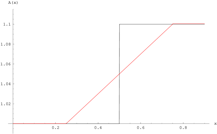
Figure 2: Example of profiles of the mean fitness functions without phenotypic fluctuation case (black); with a constant phenotypic fluctuation over a given range given by eq.(25) (red), where we set $A(x)=1+0.1\Theta(x-0.5)$ and $\ell=0.25$.

An example of $\hat{A}^{(F)}(x)$ is shown in Fig. (2). The evaluation function $f$ in section (III) is given by $f^{(F)}(x)=\hat{A}^{(F)}(x)(1-\frac{\gamma}{2}x^{2})$.

We study the case where the position ${x_{b}^{*}}^{(F)}(\equiv{x_{b}^{(F)}}(\gamma^{*}))$ is within the range $[x_{0}-\ell,x_{0}]$ because the profile of $\hat{A}^{(F)}$ shows that ${\gamma^{*}}^{(F)}$ is smaller than $\gamma^{*}_{0}$ if ${x_{b}^{*}}^{(F)}>x_{0}$. If $\frac{x_{0}}{2+A_{0}}\leq\ell<x_{0}$, the position ${x_{b}^{*}}^{(F)}$ is within the range $[x_{0}-\ell,x_{0}]$. In that case, ${\gamma^{*}}^{(F)}$ is given by ${\gamma^{*}}^{(F)}\simeq\frac{A_{0}}{4\ell(x_{0}-\ell)}$ to the first order of $A_{0}$. Comparing ${\gamma^{*}}^{(F)}$ with $\gamma^{*}_{0}$ in (24), we conclude that ${\gamma^{*}}^{(F)}<\gamma^{*}_{0}$ for $0<\ell<\frac{2+\sqrt{2}}{4}x_{0}$, and ${\gamma^{*}}^{(F)}>\gamma^{*}_{0}$ for $\frac{2+\sqrt{2}}{4}x_{0}<\ell<x_{0}$. Hence, when the half width $\ell$ of the distribution $P_{phe}$ is within the range $(\frac{2+\sqrt{2}}{4}x_{0},x_{0})$, the critical mutation rate for the error catastrophe threshold is increased. In other words, the isogenic phenotypic fluctuation increases the robustness of high fitness state against mutation.

We also studied the case in which $\hat{P}_{phe}(\bar{x},x)$ decreases linearly around its peak, i.e., with a triangular form. In this case, the phenotypic fluctuation decreases the critical mutation rate as long as $A_{0}$ is small, while it can increase for sufficiently large values of $A_{0}$, for a certain range of the values of width of phenotypic fluctuation.

V Discussion

In the present paper, we have presented a general formulation to describe the evolution of phenotype distribution. A partial differential equation describing the temporal evolution of phenotype distribution is presented with a self-consistently determined growth term. Once a microscopic model is provided, each term in this evolution equation is explicitly determined so that one can derive the evolution of phenotype distribution straightforwardly. This eq. (8) is obtained as a result of Kramers-Moyal expansion, which includes infinite order of derivatives. However, this expansion is often summed to a single term in the large number limit of base sequences, with the aid of singular perturbation.

If the value of a phenotype variable $|x|$ is much smaller than unity (which is the maximal possible value giving rise to the fittest state), the terms higher than the second order can be neglected, so that a Fokker-Planck type equation with a self-consistent growth term is derived. The validity of this truncation is confirmed by putting $x^{\prime}=(2n-N)/\sqrt{N}$ and verifying that the third or higher order moment is negligible compared with the second-order moment. Thus the equation up to its second order, (9), is relevant to analyzing the initial stage of evolution starting from a low-fitness value.

As a starting point for our formalism, we adopted eq. (2), which is called the “coupled” mutation-selection equationHofbauer . Although it is a natural and general choice for studying the evolution, a simpler and approximate form may be used if the mutation rate and the selection pressure are sufficiently small. This form given by $\frac{\partial\hat{P}(s,t)}{\partial t}=-\bar{A}(t)\hat{P}(s,t)+\sum_{s^{\prime}}Q(s^{\prime}\rightarrow s)\hat{P}(s^{\prime},t)$, is called the “parallel” mutation-selection equationkimura1970 ; Akin . It approaches the coupled mutation-selection equation (2), in the limits of small mutation rate and selection pressure, as shown in Hofbauer . If we start from this approximate, parallel mutation-selection equation, and follow the procedure presented in this paper, we obtain $\frac{\partial P(x,t)}{\partial t}=(A(x)-\bar{A}(t))P(x,t)+\gamma\frac{\partial{}}{\partial x}\left[-m_{1}^{(1)}(x)+\frac{1}{2}\frac{\partial{}}{\partial x}m_{2}^{(1)}(x)\right]P(x,t)$.

In general, this equation is more tractable than eq. (9), as the techniques developed in Fokker-Planck equations are straightforwardly applied as discussed in PhysicalBiology , and it is also useful in describing of evolution. Setting $A(x)=x^{2}$ and replacing $m_{1}^{(1)}$ and $m_{2}^{(1)}$ with some constants, the equation is reduced to that introduced by KimuraKimura2 ; while setting $A(x)=x$, $m_{1}^{(1)}(x)\propto x$, and replacing $m_{2}^{(1)}$ with some constant derives the equation by LevineLevine . Because our formalism is general, these earlier studies are derived by approximating our evolution equation suitably.

Besides the generality, another merit of our formulation lies in its use of the phenotype as a variable describing the distribution, rather than the fitness (as adopted by Kimura). Whereas the phenotype is an inherent variable directly mapped from the genetic sequence, the fitness is a function of the phenotype and environment, and strongly influenced by environmental conditions. The evaluation of the transition matrix by mutation in eq.(8) would be more complicated if we used the fitness as a variable, due to crucial dependence of fitness values on the environmental conditions. In the formalism by phenotype distribution, environmental change is feasible by changing the growth term $A(x)$ accordingly. Our formalism does include the fitness-based equation as a special case, by setting $A(x)=x$.

Another merit in our formulation is that it easily takes isogenic phenotypic fluctuation into account without changing the form of the equation, but only by modifying $A(x)$. By applying this equation, we obtained the influence of isogenic phenotype fluctuations on error catastrophe. The critical mutation rate for the error catastrophe increases because of the fluctuation, in a certain case. This implies that the fluctuation can enhance the robustness of a high-fitness state against mutation.

In fact, the relevance of isogenic phenotypic fluctuations on evolution has been recently proposedSatoPNAS ; kaneko-book ; KKFurusawaJTB , and change in phenotypic fluctuation through evolution has been experimentally verifiedIto ; SatoPNAS . In general, phenotypic fluctuations and a mutation-selection process for artificial evolution have been extensively studied recently. The present formulation will be useful in analysing such experimental data, as well as in elucidating the relevance of phenotypic fluctuations to evolution.

Figures

Appendix A Estimation of the transition probability in the NK model

In the NK modelwell-written-NK ; kauffmann-book , the fitness $f$ of a sequence $s$ is given by

$$f(s)=\frac{1}{N}\sum_{i=1}^{N}\omega_{i}(s),$$

where $\omega_{i}$ is the contribution of the $i$th site to the fitness, which is a function of $s_{i}$ and the state values of other $K$ sites. The function $\omega_{i}$ takes a value chosen uniformly from $[0,1]$ at random. We assume that the phenotype $x$ of the sequence $s$ is given by $x=f(s)$.

When $N\gg 1$, $K\gg 1$, and $K/N\ll 1$, the phenotype distribution of mutants of a given sequence $s$ (whose phenotype is $x$) is characterized only by the phenotype $x$ (without the need to specify the sequence $s$). For showing this, we first examine the one-point mutant case.

We consider the “number of changed sites” of sites at which $\omega^{\prime}s$ are changed due to a single-point mutation. By assuming that the average number of changed sites is $K$, the distribution of the number of changed sites $n$, denoted by $P_{site}(n)$, is approximately given by

$$P_{site}(n)\simeq e^{-\frac{(n-K)^{2}}{2K}},$$ (26)

with the help of the limiting form of binomial distribution. Here, we have omitted the normalization constant.

Next, we study the distribution of the difference between the phenotype $x$ of the original sequence and the phenotype $x^{\prime}$ of its one-point mutant, given the number $n$ of changed sites of the single-point mutant. We denote the distribution as $P_{dif\!f}(n;X)$, where $X=x^{\prime}-x$. Here the average of $x^{\prime}$ is $x(N-n)/N$, since $(N-n)$ sites are unchanged. Thus, according to the central limit theorem, the distribution is estimated as

$$P_{dif\!f}(n;X)\simeq\exp\left[{-\frac{(X+\frac{n}{N}x)^{2}}{2n\frac{\sigma^{2}}{N^{2}}}}\right],$$ (27)

where $\sigma^{2}$ is the variance of the distribution of the value of $\omega$. This variance is estimated from the probability distribution $P_{(s,\{\omega_{i}\})}(\omega)$ that the sequence $\omega$ is generated.. Although the explicit form of $P_{(s,\{\omega_{i}\})}$ is hard to obtain unless $\{\omega_{i}\}$ and $s$ are given, it is estimated by means of the “most probable distribution,” obtained as follows: Find the distribution that maximizes the evaluation function $S$ (called “entropy”) defined by $S=-\int_{0}^{1}P(\omega)\log P(\omega)d\omega$ under the conditions $\int_{0}^{1}P(\omega)d\omega=1$ and $\int_{0}^{1}\omega P(\omega)d\omega=x$. Accordingly the variance $\sigma^{2}$ may depend on $x$.

Combining these distributions (26) and (27) gives the distribution of $X$ without constraint on the number of changed sites:

$$P(X)=\sum_{n=1}^{N}P_{site}(n)P_{dif\!f}(n;X)\simeq\exp\left[{-\frac{(X+\frac{K}{N}x)^{2}}{2K\frac{(\sigma^{2}+x^{2})}{N^{2}}}}\right].$$

This result indicates that the phenotype distribution of single-point mutants from the original sequence $s$ having the phenotype $x$ is characterized by its phenotype $x$ only; $s$ is not necessary. Similarly, one can show that phenotype distribution of $n$-point mutants is also characterized only by $x$. Hence, the transition probability in the NK model is described only in terms of the phenotypes of the sequences, when $N\gg 1$, $K\gg 1$, and $K/N\ll 1$.

Appendix B Mathematical structure of the equation of form (9)

We first rewrite eq. (9) as

$$\frac{\partial P(x,t)}{\partial t}=-\bar{A}(t)P(x,t)+L(x)P(x,t),$$ (28)

where $L$ is a linear operator, defined by $L(x)=A(x)+\frac{\partial{}}{\partial x}f(x)+\frac{\partial{}^{2}}{\partial x^{2}}g(x)$ with $f(x)=-\gamma m_{1}^{(1)}(x)A(x)$ and $g(x)=\frac{\gamma}{2}m_{2}^{(1)}(x)A(x)$.

The linear operator $L$ is transformed to an Hermite operator using variable transformations (see below) so that $L$ is represented by a complete set of eigenfunctions and corresponding eigenvalues, which are denoted by $\{\phi_{i}(x)\}$ and $\{\lambda_{i}\}$ ($i=0,1,2,...$), respectively. Eigenvalues are real and not degenerated, so that they are arranged as $\lambda_{0}>\lambda_{1}>\lambda_{2}>...$.

According to PhysicalBiology , $P(x,t)$ is expanded as

$$P(x,t)=\sum_{i=0}^{\infty}a_{i}(t)\phi_{i}(x),$$ (29)

where $a_{i}$ satisfies

$$\frac{da_{i}(t)}{dt}=a_{i}(t)(\lambda_{i}-{\sum_{j=0}^{\infty}}^{\prime}a_{j}(t)\lambda_{j}).$$ (30)

The prime over the sum symbol indicates that the summation is taken except for those of noncontributing eigenfunctions as defined in PhysicalBiology .

Stationary solutions of eq. (30) are given by $\{a_{k}=1$ and $a_{i}=0$ for $i\neq k\}$. Among these stationary solutions, only the solution $\{a_{0}=1$ and $a_{i}=0$ for $i\neq 0\}$ is stable. Hence, the eigenfunction for the largest eigenvalue (the largest replication rate) gives the stationary distribution function. Now it is important to obtain eigenfunctions and eigenvalues of $L$, in particular the largest eigenvalue $\lambda_{0}$ and its corresponding eigenfunction $\phi_{0}$. Hence, we focus our attention on the eigenvalue problem

$$\left[A(x)+\frac{\partial{}}{\partial x}f(x)+\frac{\partial{}^{2}}{\partial x^{2}}g(x)\right]P(x)=\lambda P(x),$$ (31)

where $\lambda$ is a constant and P is a function of $x$.

We can transform eigenvalue problem (31) to a Schroedinger equation-type eigenvalue problem as follows: First we introduce a new variable $y$ related to $x$ as $y(x)=\int_{x_{0}}^{x}\sqrt{\frac{h}{g(x^{\prime})}}dx^{\prime}$ where $x_{0}$ and $h$ are constants. Next, we consider a new function $\Psi(y)$ related to $P(x)$ as

$$\Psi(y)=\left.\sqrt{\frac{g(x)}{h}}e^{{\int_{y_{0}}^{y}\frac{\hat{f}(y^{\prime})}{2h}dy^{\prime}}}P(x)\right|_{x=x(y)}$$

where $y_{0}$ is some constant, $x(y)$ the inverse function of $y(x)$, and $\hat{f}$ a function of $y$ defined by

$$\hat{f}(y)=\left.\sqrt{\frac{h}{g(x)}}(f(x)+\frac{1}{2}\frac{dg(x)}{dx})\right|_{x=x(y)}.$$

Using these new quantities $y$ and $\Psi$ and rewriting eigenvalue problem (31) suitably, we get

$$\left[V(y)+h\frac{\partial{}^{2}}{\partial y^{2}}\right]\Psi(y)=\lambda\Psi(y),$$ (32)

where $V(y)=\hat{A}(y)+\frac{\frac{d\hat{f}(y)}{dy}}{2}-\frac{\hat{f}^{2}(y)}{4h}$ with $\hat{A}(y)=A(x(y))$.

References

- (1) S. F. Elena and R. E. Lenski, Nat. Rev. Genet. 4, 457 (2003).
- (2) R. E. Lenski, M. R. Rose, S. C. Simpson, and S. C. Tadler, Am. Nat. 183, 1315-1341 (1991).
- (3) M. Hegreness, N. Shoresh, D. Hartl, and R. Kishony, Science 311, 1615 (2006).
- (4) A. E. Mayo, Y. Setty, S. Shavit, A. Zaslaver, and U. Alon, PLoS Biol. 4, 556-561 (2006).
- (5) E. Dekel and U. Alon, Nature 436, 588-592 (2005).
- (6) A. Kashiwagi, W. Noumachi, M. Katsuno, M. T. Alam, I. Urabe, and T. Yomo, J. Mol. Evol. 52, 502-509 (2001).
- (7) Y. Ito, T. Kawama, I. Urabe, and T. Yomo, Mol. Evol. 58(2), 196-202 (2004).
- (8) A well established theory in population genetics, which adopts diffusion equation or Fokker-Planck type equation, is related to the frequency of genes in alleles in population as developed by Wright, Fisher, and KimuraFisher ; Wright ; kimura1970 . How new genes spread in population is analyzed by the diffusion equation. In contrast, we are concerned with the changes in the distribution of a base sequence consisting of a haploid gene.
- (9) R. A. Fisher, Proc. Roy. Soc. Edinb. 50, 205 (1930); The genetical theory of natural selection (Oxford University Press, Oxford, 1999).
- (10) S. Wright, Proc. Natl. Acad. Sci. USA 31, 382 (1945); The theory of gene frequencies (University of Chicago Press, Chicago, 1969).
-
(11)
J. F. Crow and M. Kimura, An introduction to population genetics theory
(Harper
&Row, New York, 1970). - (12) M. Kimura, Proc. Natl. Acad. Sci. USA 54, 731-736 (1965).
- (13) L. S. Tsimring, H. Levine, and D.A. Kessler, Phys. Rev. Lett. 76, 4440 (1996).
- (14) M. Eigen, J. McCaskill, P. Schuster, J. Phys. Chem. 92, 6881-6891 (1988).
- (15) S. Kauffman, The Origins of Order (Oxford University Press, New York, 1993).
- (16) J. Spudich and D. Koshland, Nature 262, 467-471 (1976).
- (17) M. B. Elowitz, A. J. Levine, E. D. Siggia, and P. S. Swain, Science 297, 1183 (2002).
- (18) M. Kaern, T. C. Elston, W. J. Blake, and J.J. Collins, Nat. Rev. Genet. 6, 451-464 (2005).
- (19) J. Hasty, J. Pradines, M. Dolnik, and J. J. Collins, Proc. Natl. Acad. Sci. USA 97, 2075-2080 (2000).
- (20) C. Furusawa, T. Suzuki, A. Kashiwagi, T. Yomo, and K. Kaneko, BIOPHYSICS 1, 25 (2005).
- (21) M. Ueda, Y. Sako, T. Tanaka, P. Devreotes, and T. Yanagida, Science 294, 864 (2001).
- (22) A. Bar-Even, J. Paulsson, N. Maheshri, M. Carmi, E. O’Shea, Y. Pilpel, and N. Barkai, Nat. Genet. 38, 636-643 (2006).
- (23) K. Sato, Y. Ito, T. Yomo, and K. Kaneko, Proc. Nat. Acad. Sci. USA 100, 14086 (2003).
- (24) K. Kaneko, Life: An Introduction to Complex Systems Bioilogy (Springer, Berlin, 2006).
- (25) K. Kaneko and C. Furusawa, J. Theo. Biol. 240, 78-86 (2006).
- (26) L. W. Ancel, Theor. Popul. Biol. 58, 307-319 (2000).
- (27) N. G. van Kampen, Stochastic processes in physics and chemistry (North-Holland, Amsterdam, 1992).
- (28) R. Kubo, K. Matsuo, and K. Kitahara, J. Stat. Phys. 9, 51 (1973).
- (29) E. Baake and H. Wagner, Genet. Res. 78, 93-117 (2001).
- (30) M. S. Waterman, Introduction to computational biology : maps, sequences and genomes (Chapman and Hall, London, 1995).
- (31) C. Furusawa, K. Kaneko, Phys. Rev. E 73, 011912 (2006).
- (32) J. H. Gillespie, Theor. Popul. Biol. 23, 202-215 (1983).
- (33) H. A. Orr, Evolution 56, 1317-1330 (2002).
- (34) H. Haken, Synergetics: an introduction nonequilibrium phase transitions and self-organization in physics, chemistry and biology (Springer-Verlag, Berlin, 1978).
- (35) K. Sato and K. Kaneko, Phys. Biol. 3, 74-82 (2006).
- (36) P. M. Morse and H. Feshbach, Methods of theoretical physics (McGraw-Hill, New York, 1953), pp. 1092-1106.
- (37) I. Leuthausser, J. Stat. Phys. 48, 343-360 (1987).
- (38) E. Baake, M. Baake and H. Wagner, Phys. Rev. Lett. 78, 559 (1997).
- (39) D. B. Saakian and C. K. Hu, Proc. Natl. Acad. Sci. USA 103, 4935-4939 (2006).
- (40) D. Saakian and C. K. Hu, Phys. Rev. E 69, 021913 (2004).
- (41) H. Yang, G. Luo, P. Karnchanaphanurach, T. M. Louie, I. Rech, S. Cova, L. Xun, and X. S. Xie, Science 302, 262-266 (2003).
- (42) L. W. Ancel and W. Fontana, J. Exp. Zool. 288, 242-283 (2000).
- (43) J. Hofbauer, J. Math. Biol. 23, 41-53 (1985).
- (44) E. Akin, The geometry of population genetics (Springer-Verlag, Berlin, 1979).
- (45) B. Levitan and S. Kauffman, Mol. Divers. 1, 53-68 (1995).