Function Constrains Network Architecture and Dynamics: A Case Study on the Yeast Cell Cycle Boolean Network

Abstract

We develop a general method to explore how the function performed by a biological network can constrain both its structural and dynamical network properties. This approach is orthogonal to prior studies which examine the functional consequences of a given structural feature, for example a scale free architecture. A key step is to construct an algorithm that allows us to efficiently sample from a maximum entropy distribution on the space of boolean dynamical networks constrained to perform a specific function, or cascade of gene expression. Such a distribution can act as a “functional null model” to test the significance of any given network feature, and can aid in revealing underlying evolutionary selection pressures on various network properties. Although our methods are general, we illustrate them in an analysis of the yeast cell cycle cascade. This analysis uncovers strong constraints on the architecture of the cell cycle regulatory network as well as significant selection pressures on this network to maintain ordered and convergent dynamics, possibly at the expense of sacrificing robustness to structural perturbations.

I Introduction

A central problem in biology involves understanding the relationship between structure and function. This problem becomes especially intricate in the era of systems biology in which the objects of study are biological networks composed of large numbers of interacting molecules. To what extent does the structure of a biological network constrain the range of functions, or types of dynamical behaviors, that the network is capable of producing? Conversely, to what extent does the requirement of carrying out a specific function constrain the structural and more general dynamical properties of a network?

There already exists a large body of theoretical work addressing the former question. For example Kauffman Kauffman and others performed an extensive study of ensembles of simplified boolean networks with fixed structural properties, such as the number of nodes and the mean degree of connectivity. A principal finding was a phase transition in the resulting dynamical behavior, from ordered to chaotic, as the connectivity increased Ald . More recently, the observation that many biological networks are scale free spurred a flurry of research into the dynamical consequences of the scale free structural feature JeoTomAlbOltBar ; AldClu ; JeoMasBarOlt ; MasSne ; OikClu . A principal finding was that the scale-free architecture is more robust to random failures and dynamic fluctuations, and may be more evolvable.

Alternatively, the latter question involving the structural and dynamical consequences of performing a specific function remains relatively unexplored Wag05 ; MaLai ; KasAlo . It is an important question because many biological functions are performed by relatively small network modules for which gross statistical properties such as mean connectivity, or any kind of degree distribution, scale free or not, do not have a clear significance. A key example of such a module is the yeast cell cycle control network, whose essential function was reduced to the boolean dynamics of a set of 11 nodes by Li, et. al. LiLonLuOuyTan . Despite the small network size, a dynamical analysis of this simple model demonstrated a great deal of robustness of the cell cycle trajectory to both fluctuations in protein states and perturbations of network structure. Is this robustness carefully selected for through evolution and encoded somehow in the topological structure of the cell cycle network, or does it arise for free, simply as a consequence of the functional constraint of having to produce the long cascade of gene expression that controls the cell cycle?

In this paper we develop techniques to address this question, and more generally to address the consequences of specific functional, rather than structural constraints. A key step in the above work exploring the dynamical consequences of fixed structural constraints was the ability to efficiently sample from the maximum entropy distribution on the space of networks constrained to have a fixed structural feature, such as a given degree distribution. We call such an ensemble a structural ensemble. Similarly, in order to address the structural consequences of fixed functional constraints, we develop an efficient algorithm to sample from a maximal entropy distribution on the space of biological networks constrained to perform a specific function. We call the resulting ensemble of networks a functional ensemble.

Since we use a maximal entropy distribution, which introduces no further assumptions about the network other than the fact that it performs a given function, we can use such functional ensembles to test whether any dynamical or structural property of a given biological network is simply a consequence of the function it performs, or rather a consequence of further selection. Under this functional null model, statistically significant properties of a real biological network can give us insight into additional selective pressures that have operated on that network above and beyond the baseline functional requirements. As an illustration of this general method, we focus on the specific case of the cell cycle network of LiLonLuOuyTan , uncovering deeper insight into the evolutionary pressures on its structural and dynamical properties.

II Methods

II.1 The Dynamical Model

We consider a simplified, boolean model of biological network dynamics, in which each degree of freedom, or node $s_{i}$, $i=1\dots N$ takes one of two values at any given time: either 0 (inactive) or 1 (active). For example, the two values could signify whether a protein is expressed or not, or whether a kinase is activated or not. Thus the full state at time t is captured by a column vector

$${\bf S}(t)=(s_{1}(t),s_{2}(t),\ldots,s_{N}(t))^{T}$$ (1)

that can take one of $2^{N}$ values. Time progresses in discrete steps, and the nodes can either activate or inhibit each other at the next step. These interactions are captured by the network connectivity matrix C with elements $c_{ij}$ representing an interaction arrow from node $j$ to node $i$. The allowed values of $c_{ij}$ are given by

$$c_{ij}\in[-1,0,1].$$ (2)

For two (possibly identical) nodes $i$ and $j$, if $c_{ij}$ is nonzero, it can be either activating (+1) or inhibiting (-1). This terminology is justfied by the dynamical rule

$$s_{i}(t+1)=f_{i}({\bf C},{\bf S}(t)),$$ (3)

where

$$f_{i}({\bf C},{\bf S}(t))=\left\{\begin{array}[]{ll}1,&\sum_{j}c_{ij}s_{j}(t)>0\\ 0,&\sum_{j}c_{ij}s_{j}(t)<0\\ s_{i}(t),&\sum_{j}c_{ij}s_{j}(t)=0.\end{array}\right.$$ (4)

Essentially, if the total input to a node is positive (negative), it will be on (off) at the next time step. In the case of zero input, the node maintains its state.

II.2 Generating Functional Ensembles

A biological network achieves its function by successfully taking the values of its nodes through a sequence of states. Thus we will equate the notion of function with a specified state trajectory

$${\bf S}(0)\rightarrow{\bf S}(1)\rightarrow\cdots\rightarrow{\bf S}(T).$$ (5)

In our example of the cell cycle network, the state sequence is simply the natural cell cycle trajectory. We wish to either enumerate or uniformly sample from the space of networks, or equivalently connectivity matrices ${\bf C}$, that can successfully perform the above sequence of $T$ state transitions. We can think of each of the $T$ transitions as providing one constraint on the connectivity matrix ${\bf C}$ via the dynamical rule given by equations (3) and (4). Assuming the nodes are distinguishable, the number of networks, given by the number of allowed connectivity matrices is $M\equiv 3^{N^{2}}$. Even for small, mesoscopic scale networks such as the cell cycle with 11 nodes, $M\approx 5.39\times 10^{57}$ and so it is computationally infeasible to iterate through all of these networks and find those for which the $T$ constraints corresponding to the $T$ transitions in (5) are satisfied. Even if one were to sample from these $M$ networks, one would rarely find a network that could perform the function in (5).

However, it is important to note that the constraint on the network connectivity ${\bf C}$ imposed by a given transition actually decouples across the rows of the connectivity matrix. That is for each node $i$, the dynamical rule in Eq. (4) depends only on the $i$’th row $c_{ij},j=1\dots N$ of ${\bf C}$, or equivalently on the $N$ incoming interaction arrows whose target is node $i$. Thus we can check that the $T$ constraints induced by the target sequence (5) are satisfied for each row, independently of the other rows. For any given $i$, the number of possible rows is $Z\equiv 3^{N}$, which is 177,147 for the yeast cell cycle network. Thus it becomes computationally feasible to exhaustively iterate through all possible row values, or incoming arrow combinations, for each node, and check that the $T$ constraints are satisfied for each such combination.

After following this procedure using the cell-cycle process as the constraint, let $1\leq\alpha_{i}\leq Z$ index the set of allowed incoming arrow combinations to node $i$ that satisify all constraints. If for each node $i$, we uniformly choose a particular $\alpha_{i}$, and assemble the corresponding $N$ allowed rows into a matrix $C$, we will have constructed a network that can successfully carry out the state trajectory in (5). This is essentially our sampling procedure. It produces a functional ensemble: a maximum entropy distribution on the space of networks constrained to produce the function represented by (5).

II.3 Combined structural and functional ensembles.

In order to perform a more fine scale study of the properties of the yeast cell cycle network, we wish to constrain more than just a predefined function. We would also like to understand how various properties depend on the number of nonzero interaction arrows in the network. Thus we need to develop a method to uniformly sample from the space of networks that both perform a fixed function and have a fixed number of arrows. However, although the algorithm presented in the previous section uniformly samples the space of networks performing a fixed function, when one adds a constraint on the number of arrows, this algorithm performs a biased sampling of the more constrained space of networks.

To see the origin of this bias, consider an implementation of the algorithm. Let $A$ be the desired number of arrows in the network. Fix an arbitrary ordering of the nodes $i=1\dots N$. Choose node 1 and pick at random one incoming arrow combination from a uniform distribution on the allowed incoming arrow combinations to node 1. Let $a_{1}$ be the number of nonzero interaction arrows in the chosen combination. We then have $A-a_{1}$ incoming arrows left to distribute to nodes $2\dots N$. If the algorithm continues in this way all the way to node $N$, one can see that the resulting sampling of networks is biased in such a way that earlier nodes in the order have a higher likelihood of receiving more incoming arrows relative to later nodes. For example, in the extreme case, the algorithm may run out of arrows even before it reaches the final node $N$. To correct for this bias, at each step of the algorithm corresponding to each node $i$ we must sample nonuniformly from a certain conditional distribution on the allowed incoming arrow combinations to node $i$.

We perform this nonuniform sampling as follows. Suppose that by the time we have reached node $i$, we have $r_{i}$ incoming arrows left to distribute among the remaining nodes from $i\dots N$. By definition, $r_{1}=A$, the number of desired arrows in our ensemble. To choose a particular incoming arrow combination to node $i$, we first randomly draw the number of incoming arrows $a_{i}$ we wish to assign to node $i$ from a conditional probability distribution $P_{i}(a_{i}|r_{i})$. Then we draw the particular combination from a uniform distribution on the set of allowed incoming arrow combinations that have exactly $a_{i}$ nonzero arrows. $P(a_{i}|r_{i})$ is a conditional distribution on the number of nonzero incoming arrows to node $i$, conditioned on the total number of incoming arrows to the remaining unassigned nodes $i\dots N$, and it can be computed as follows. Let $W_{i}(a_{i})$ be the number of allowed incoming arrow combinations to node $i$ that have exactly $a_{i}$ nonzero arrows. Let $Q_{i+1}(b)$ be the number of ways to distribute $b$ incoming arrows (consistent with the fixed function the network must perform) to the remaining nodes $i+1\dots N$. Then for each choice $a_{i}$ of the number of incoming arrows to node $i$, the quantity $W_{i}(a_{i})Q_{i+1}(r_{i}-a_{i})$ is the number of allowed ways to complete the network. $P(a_{i}|r_{i})$ is simply proportional to this number:

$$P_{i}(a_{i}|r_{i})=\frac{W_{i}(a_{i})Q_{i+1}(r_{i}-a_{i})}{\sum_{b=0}^{min(N,r_{i})}W_{i}(b)Q_{i+1}(r_{i}-b)},\quad i=1\dots N-1.$$ (6)

Intuitively, the combinatoric factor $Q_{i+1}(r_{i}-a_{i})$ in the definition of of the conditional distribution $P_{i}(a_{i}|r_{i})$ corrects for the biased sampling mentioned above by forcing the algorithm to choose uniformly from the set of possible completions of the network, rather than simply uniformly from the set of allowed incoming arrows to node $i$. For the special case of the last node $i=N$, when we have $r_{N}$ arrows left to distribute, we simply choose uniformly from the allowed space of incoming arrow combinations to node $N$ that have exactly $r_{N}$ nonzero arrows. Furthermore, each time we run the algorithm to obtain a network, we randomize the ordering on the nodes.

For any fixed ordering of the nodes, the combinatoric factors $Q_{i}(b)$ are crucial to the success of the sampling algorithm. We note that these factors can be computed efficiently by working recursively from node $i=N$ back down to $i=1$. More precisely, if we define

$$Q_{N}(b)\equiv W_{N}(b),$$ (7)

then for each $i=1\dots N-1$ we have the recursion relation

$$Q_{i}(b)=\sum_{a=0}^{min(N,b)}W_{i}(a)Q_{i+1}(b-a).$$ (8)

Thus this algorithm gives us an efficient way to sample from a combined structural and functional ensemble: a maximum entropy distribution on the space of networks constrained to have a fixed function and a fixed number of arrows. It is this algorithm that we use to generate the ensemble of “cell cycle” networks described below. In order to compare this ensemble to a set of more random networks that serve no particular function, we generated this “random network” ensemble by randomly rewiring the connections in each “cell-cycle” network under the constraint that all nodes must be connected to the same network, i.e. no isolated nodes or sub-networks.

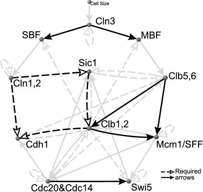
Figure 1: Simplified yeast cell-cycle network from Li et al. LiLonLuOuyTan . Each node represents a gene or its protein product that participates in the regulation of the yeast cell-cycle. There are cyclins (Cln1,2, Cln3, Clb1,2, Clb5,6), transcription factors (SBF, MBF, Mcm1/SFF, Swi5), and factors that inhibit or degrade cyclins (Sic1, Cdh1, Cdc20). Solid and dashed arrows are activating and deactivating interactions, respectively. The black solid and black dashed arrows are absolutely required for a network to produce the cell-cycle process [see Table 1].

Table 1: The cell-cycle process generated by the simplified yeast cell-cycle network in Fig. 1.

Time	Cln3	MBF	SBF	Cln1,2	Clb5,6	Clb1,2	Mcm1	Cdc20	Swi5	Sic1	Cdh1	Phase
1	1	0	0	0	0	0	0	0	0	1	1	“Excited” G1
2	0	1	1	0	0	0	0	0	0	1	1	G1
3	0	1	1	1	0	0	0	0	0	1	1	G1
4	0	1	1	1	0	0	0	0	0	0	0	G1
5	0	1	1	1	1	0	0	0	0	0	0	S
6	0	1	1	1	1	1	1	0	0	0	0	G2
7	0	0	0	1	1	1	1	1	0	0	0	M
8	0	0	0	0	0	1	1	1	1	0	0	M
9	0	0	0	0	0	1	1	1	1	1	0	M
10	0	0	0	0	0	0	1	1	1	1	0	M
11	0	0	0	0	0	0	0	1	1	1	1	M
12	0	0	0	0	0	0	0	0	1	1	1	G1
13	0	0	0	0	0	0	0	0	0	1	1	Stationary G1

III The yeast cell-cycle network

The simplified yeast cell-cycle Boolean network [see Fig. 1] given in Li et al. LiLonLuOuyTan contains 11 proteins, or nodes, and 1 checkpoint. There are 34 arrows connecting the nodes: 15 activating and 19 deactivating (“self-degrading” arrows are equivalent to deactivating arrows under our dynamical model). Using the above dynamical model, this network can produce the cell-cycle process, as shown in Table 1. Starting from the “excited” G₁ state, the process goes through the S phase, the G₂ phase, the M phase, and finally returns to the biological G₁ stationary state. The network also has 7 fix-points, with the G₁ stationary state being the biggest, having a basin size of 1764 ($\approx$ 86% of all protein states).

IV Results

We used the same 11 nodes and the types of connections in the simplified yeast cell-cycle Boolean network to construct our ensembles of networks. Using our technique to generate purely functional ensembles, we were able to select 11 sets of inward connection combinations (one for each node) that produce the cell-cycle process [see Table 1]. Figure 2 shows the compositions of different types of connections in the sets. The number of selected connection combinations for each node (shown in parenthesis in Fig. 2) varies for two orders of magnitude. The number of networks that can realize the cell-cycle process is $5.11\times 10^{34}$ and the distribution against the number of arrows is shown in Fig. 3.

IV.1 Constraints on Structure from Function.

From Fig. 2 we can deduce that there are 10 core connections (shown as black solid and black dashed arrows in Fig. 1) that are absolutely required in order to produce the cell-cycle process. These required connections become obvious once we look closer into the cell-cycle process. For example, comparing the $G_{1}$ stationary state and the “excited” $G_{1}$ state, Cln3 is the only node that is turned on; this implies that MBF and SBF, which are turned on in the next time step, can only be activated by Cln3. The remaining required connections can all be deduced using the same logic. The compositions of different connection types follow a common trend where there is a higher chance for a node to be positively regulated by nodes that are active earlier in the cell-cycle process (positive feed-forward) and negatively regulated by nodes that are active later in the process (negative feedback) [see Fig. 4]. This trend seems to be general for networks that produce cascades of activation. To check this, we looked at the connection compositions for two simple activation cascades, where 11 nodes are activated in turn for 4 or 5 time steps, and they indeed show the same trend [See Table 2 and Fig. 5 for 5 time steps activation cascade].

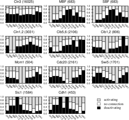
Figure 2: Fractions of different types of inward connections to each node from all other nodes (including itself) that produce the cell-cycle process [see Table 1]. Numbers in parenthesis are the number of connection combinations selected by our algorithm [see Methods].

Figure 3: Distribution of number of networks that can realize the cell-cycle process over the number of arrows in the networks.

Figure 4: Positive feed-forward and negative feedback connections between network nodes. Solid and dashed arrows are the most probable activating and deactivating interactions, respectively, selected from Fig. 2. The activating arrow for Cln3 is not a clear winner, therefore colored gray. Nodes are placed in the order of their activation in the cell-cycle process, starting from Cln3 and continues clockwise, SBF and MBF turn on at the same time, and similarly for Mcm1/SFF and Clb1,2. Positive feed-forward interactions connecting Cln3 to Cln1,2, Cln3 to Clb5,6 and Clb5,6 to Mcm1/SFF can be seen. Negative feedback connections from later nodes to earlier nodes are also obvious. These interactions will be more common when more arrows are added. This network (less the gray arrow) does not produce the cell-cycle process but one very close to it.

Table 2: A simple activation cascade with 11 nodes activated in turn for 5 time steps

Time	A	B	C	E	F	G	H	I	J	K	L
1	1	0	0	0	0	0	0	0	0	0	0
2	1	1	0	0	0	0	0	0	0	0	0
3	1	1	1	0	0	0	0	0	0	0	0
4	1	1	1	1	0	0	0	0	0	0	0
5	1	1	1	1	1	0	0	0	0	0	0
6	0	1	1	1	1	1	0	0	0	0	0
7	0	0	1	1	1	1	1	0	0	0	0
8	0	0	0	1	1	1	1	1	0	0	0
9	0	0	0	0	1	1	1	1	1	0	0
10	0	0	0	0	0	1	1	1	1	1	0
11	0	0	0	0	0	0	1	1	1	1	1
12	0	0	0	0	0	0	0	1	1	1	1
13	0	0	0	0	0	0	0	0	1	1	1
14	0	0	0	0	0	0	0	0	0	1	1
15	0	0	0	0	0	0	0	0	0	0	1
16	0	0	0	0	0	0	0	0	0	0	0

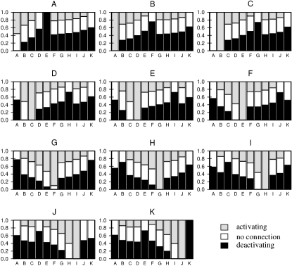
Figure 5: Fractions of different types of inward connections to each node from all other nodes (including itself) that produce the activation cascade in Table 2.

Next, we generated two network ensembles for each number of arrows allowed in the space of cell cycle networks. This number of arrows varied from 24 to 117 as seen in Fig. 3. The first ensemble is a combined structural/functional ensemble [see Methods] consisting of 1,000 networks that both realize the cell cycle and have a fixed number of arrows. These networks will be referred to as the “cell-cycle networks” (CN). The second ensemble was generated by randomly reconnecting the arrows for each network in the first ensemble [see Methods]. This ensemble will be referred to as the “random networks” (RN).

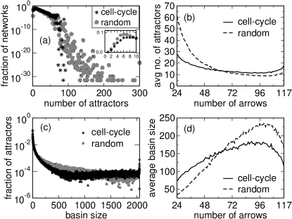
Figure 6: Number of attractors and basin sizes of attractors for the two ensembles of networks. (a) Distribution of number of attractors. Inset shows the distribution for $\leq$ 10 attractors (b) Number of attractors averaged over networks with the same number of arrows. (c) Distribution of size of basins of attractions. (d) Basin size averaged over networks with the same number of arrows.

IV.2 Analysis of Attractors: Large Basins for Free

We studied the time evolution of protein states of the two ensembles by using the dynamical model described in the Methods and initiating the networks from each of the $2^{11}=2,048$ states. We found that the CN networks have fewer attractors and larger attractor basin sizes compared to the RN networks [see Fig. 6 (a),(c)]. The number of attractors decreases as the number of arrows increases, reaching a minimum at around 100 arrows and then increases again [see Fig. 6 (b)]. The two curves cross each other at about 60 arrows, therefore, compared to RN networks, CN networks have fewer attractors when the number of arrows is small and more attractors when the number of arrows is large. The behavior is reversed for the size of attractor basins [see Fig. 6 (d)]. In the CN ensemble, the probabilities for a network with 34 arrows to have $\leq$ 7 attractors and to have the biggest attractor basin size $\geq$ 1764 (as in the case of yeast cell-cycle network) are 4.1% and 7.5% respectively. In the RN ensemble the corressponding percentages are only 1.5% and 0.7% respectively. Thus we see that the constraint of having to perform the yeast cell cycle cascade alone can, to a certain extent, help explain the origins of these two measures of dynamical robustness; a large basin essentially arises for free as a consequence of the cell cycle function. Indeed, the average basin size of the biggest attractors for the CN ensemble is 1397 compared to 1045.53 for the RN ensemble. In addition, 95.3% of the networks in the CN ensemble have the $G_{1}$ stationary state as the biggest attractor and the average basin size of these attractors is 1536.92.

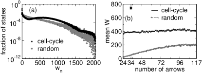
Figure 7: (a) Distribution of convergence value $w_{n}$ for network states in each ensemble. (b) Overall convergence $W$ averaged over networks with the same number of arrows. Error bar represent one standard error.

IV.3 Convergence of Trajectories.

Following LiLonLuOuyTan , we define a measure $w_{n}$ that quantifies the “degree of convergence” of the dynamical network trajectories onto each network state $n$ where $n=1,\dots,2048$. Let $T_{j,k}$ denote the number of trajectories starting from all 2048 initial network states that travel from state $j$ to state $k$ in one time step. Let $L_{n}$ denote the number of steps it takes to get from state $n$ to its attractor, so that we can index the states along the outward trajectory by $k=1,\dots,L_{n}$. Then $w_{n}=\sum_{k=1}^{L_{n}}T_{k-1,k}/L_{n}$. The overall convergence, or overlap $W$ of trajectories is given by the average of $w_{n}$ over all states $n$.

The distribution of the $w_{n}$ values is shown in Fig. 7 (a). The result shows that there are more states in the CN ensemble having larger $w_{n}$ values indicating a higher degree of convergence in the network dynamics. The local maxima at $w_{n}=559$ for this ensemble should be a result of the requirement that networks in this ensemble must produce the cell-cycle process. The overall overlap $W$ [see Fig. 7 (b)], which is the average of $w_{n}$ over all network states, for the yeast cell-cycle network is 743 and the probability for a network with 34 arrows in the CN ensemble to have $W\geq 743$ is 3.1%. Such a result is highly unlikely in the RN ensemble. In fact no networks in the RN ensemble with 34 arrows had an overlap $W\geq 743$. Thus a higher degree of convergence is a dynamical consequence of performing the cell cycle function, but nevertheless, the actual cell cycle network in Fig. 1 still displays a relatively high degree of convergence even within the CN ensemble. The statistical significance of the yeast cell cycle’s overlap parameter $W$ within the functional cell cycle ensemble suggests the existence of a strong selection pressure for convergent dynamics.

Figure 8: Distribution of transient times.

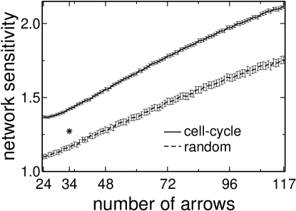
Figure 9: Network sensitivity averaged over networks with the same number of arrows. Asterisk ($\ast$) shows the network sensitivity of the yeast cell-cycle network. Error bar represent four times standard error.

IV.4 Dynamical Order: Transients and Sensitivity.

To compare the degree of order between the networks in the two ensembles, we calculated the transient time for all network states for all networks [see Fig. 8]. The transient time is defined as the amount of time for a network state to evolve to its attractor, which is equal to the length of its trajectory Wuensche . The result shows that CN networks have longer transient times and thus are more chaotic than RN networks (unless the RN networks have long attracting limit cycles). The average transient time for the yeast cell-cycle network is 7.47, and the probability for a cell-cycle network with 34 arrows to have $\geq 7.47$ average transient time is 4.8%.

We then calculated the network sensitivity $s$ ShmuKau for all networks [see Fig. 9]. Network sensitivity is the average expected number of node state changes in the output given a one node state change in the input. In other words, $s$ calculates the average hamming distance of the output states of the network for all hamming neighbor input states (i.e. hamming distance = 1). If $s<1$, the network is ordered; fluctuations in node states die out quickly and remain localized. If $s>1$, the network is “chaotic”; fluctuations are amplified at least on short time scales. On longer time scales, which are not captured, especially for small networks, by this one step measure of sensitivity, the network may not be chaotic and could still converge to a stable fixed point. When $s=1$, the network is in some sense critical.

The result in Fig. 9 indicates that networks in both ensembles are on average chaotic, or more precisely, display a significant degree of short time scale sensitivity to input perturbations, for any number of arrows within the range we studied. The sensitivity $s$ increases monotonically with the number of arrows in a network. The values of s for the RN ensemble remain smaller than those for the CN ensemble demonstrating that CN networks are indeed more chaotic, or sensitive to input perturbations, than RN networks. The yeast cell-cycle network has a network sensitivity of 1.27, which is more ordered on average than other members in its ensemble. Indeed the probability for a network with 34 arrows in the CN ensemble to have $s\leq 1.27$ is only 3.1%. Thus the actual cell cycle is remarkably ordered, or insensitive to input perturbations, despite the fact that the functional constraint of performing the cell cycle drives networks to be more sensitive to such perturbations on short time scales.

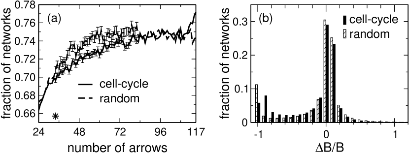
Figure 10: Response to perturbations to network structure. (a) Fractions of perturbed networks, for each number of arrows, that retain the original biggest attractor. Asterisk ($\ast$) shows the fraction for the perturbed yeast cell-cycle network. Error bars represent one standard error. (b) Distribution of relative changes of the size of the basin of attraction for the biggest attractor.

IV.5 Dynamical response to structural perturbations.

To check and compare how the networks respond to structural perturbations, we performed the same kinds of alterations described in Li et al. LiLonLuOuyTan on all networks in the two ensembles. The alterations included deleting arrows from, adding arrows to and switching the signs of arrows in the networks. We assessed the response by calculating the percentage of perturbed networks that retain their original biggest attractor [see Fig. 10 (a)] and also the relative change in the size B of the basin of attraction for the original biggest attractors [see Fig. 10 (b)]. The percentages of perturbed networks in the two ensembles that retain their original biggest attractor both increase initially when the number of arrows in the network is small. The percentages are similar when there are about 24 to 33 arrows in the networks but as the number of arrows exceeds 33, the percentage for the RN ensemble becomes significantly greater compared to that for the CN ensemble. The two percentage become similar again when the number of arrows increases beyond 83 and separate once more at 144 arrows but the percentage for CN ensemble is greater this time. The percentage for yeast cell-cycle network (65.7%) is smaller than the average for CN networks with the same number of arrows. The probability to obtain an equal or higher percentage is 80.7%, indicating that the yeast cell-cycle network has a worse than average robustness with respect to such structural perturbations.

We noticed from the distributions of ${\Delta}B/B$ that there is a higher chance for perturbations to have a deleterious effect to networks in the CN ensemble where the change in the sizes of basins of attraction is usually negative. However, there is a much higher chance for networks in the RN ensemble to completely lose the original biggest attractor (${\Delta}B/B=-1$), which is even more unfavorable. The above effects should be attributed to the smaller basins of attraction for networks in the RN ensemble. The average ${\Delta}B/B$ for yeast cell-cycle network is -0.342 and the probability for a CN network with 34 arrows to have average ${\Delta}B/B$ value $\geq-0.342$ is 89%. This again signifies a worse than average robustness for the yeast cell-cycle network.

Figure 11: Fractions of trajectories of the perturbed networks starting from the “excited” $G_{1}$ state that still evolve to the biological $G_{1}$ stationary state and fraction of cell-cycle processes of the perturbed networks remain unchanged. Asterisk ($\ast$) and cross (x) show the fraction of trajectories reaching $G_{1}$ stationary state and fraction of cell-cycle processes unchanged, respectively, for perturbed yeast cell-cycle networks. Error bars reprensent four times standard error.

IV.6 Stability of the cell cycle process.

Finally, we checked how many perturbed networks from the CN ensemble could still maintain the cell-cycle process [see Fig. 11]. Starting from the “excited” $G_{1}$ state, the fraction of trajectories reaching the $G_{1}$ stationary state and the fraction of cell-cycle processes unchanged increase as the number of arrows in the network increases. The fraction of trajectories reaching the $G_{1}$ stationary state and the fraction of cell-cycle processes unchanged for the yeast cell-cycle network are 0.52 and 0.22 respectively. The probability for a CN network with 34 arrows to maintain $\geq 52$% of trajectories reaching the $G_{1}$ stationary state and $\geq 22$% of cell-cycle processes unchanged are 79% and 61.2% respectively.

V Discussion

We presented a maximum entropy analysis method that can reveal the underlying structural constraints, as well as the statistical significance of various dynamical properties, of networks that perform a certain function. We applied this method to the yeast cell-cycle network and the accompanying cell-cycle process LiLonLuOuyTan .

We demonstrated that requiring a network to produce an activation cascade, e.g. the cell-cycle process, requires the network to have positive feed-forward and negative feedback interactions between their nodes. It is not just the case that this is a good design principle to realize a long transient cascade; it is essentially the only way to achieve it generically, and yields an example of how network function constrains network structure.

We also showed that certain dynamical features arise purely as a consequence of performing the cell-cycle function. Compared to the random (RN) ensemble, networks in the cell-cycle (CN) ensemble had much larger basins of attraction, a higher degree of convergence of trajectories, longer transient times, and more chaotic behavior on short time scales, as measured by the network sensitivity $s$. These properties may be essential for networks to produce a long sequence of state transitions. The long trajectory of the cell-cycle process provides many possible merge points for other trajectories, which certainly contribute to the high degree of convergence in the network dynamics and the large basin of attraction for $G_{1}$ stationary state. Thus the existence of this globally attracting trajectory of the dynamics alone can explain to a certain extent the observed robustness against dynamical perturbations over long time scales.

On the other hand, with respect to structural perturbations, the actual yeast cell cycle is relatively less robust compared to other networks in the CN ensemble. This is in stark contrast to the high degree of dynamical order on short time scales displayed by the cell cycle network, which suggests that there may be a trade off between ordered dynamics and structural robustness. The network sensitivity ShmuKau , which measures the degree of order, calculates how sensitive a network is to fluctuations in the states of the nodes, which is a major source of variation in a cell population EloLevSigSwa ; RasOShea1 ; RasOShea2 ; SwaEloSig . Evolution may have favored a design for the yeast cell-cycle network that is ordered and less sensitive to fluctuations in the states of the nodes (e.g. it has been reported that there is on average only 1 copy of SWI5 mRNA per cell in yeast Holland ), by sacrificing robustness against perturbations to the network structure. However, we expect that the complete yeast cell-cycle network is more robust against such perturbations since it has “redundant” components and connections that perform similar jobs.

In any case, the observation that only 3.1% of randomly chosen cell cycle networks with 34 arrows are more ordered (as measured by the sensitivity $s$) than the real cell cycle network reveals an unsuspected but significant selection pressure for short time scale ordered dynamics that cannot be explained by the functional requirement of maintaining the cell cycle process; indeed the functional requirement of maintaining the cell cycle proccess forces the dynamics in the opposite direction, i.e. to be more chaotic on short time scales. Similarly, we have seen that simply requiring a long cell cycle to occur automatically raises the average degree of convergence of trajectories over longer time scales. However, even after accounting for this increase within the functional ensemble, only 3.1% of all cell cycle networks with 34 arrows have a greater degree of convergence (as measured by the overlap parameter $W$), reflecting an evolutionary pressure for convergent dynamics on long time scales above and beyond that necessitated by the requirements of the cell cycle function alone.

Although we have focused on a single biological example, the cell cycle, our analysis method is quite general. It would be interesting to perform it on other mesoscopic scale networks that have a comparable number of components to uncover their structural and dynamical constraints. More generally, we believe these techniques of simultaneously analyzing both structural and functional ensembles of networks will prove useful in the larger quest to deduce general principles governing relations between structure, dynamics, function, robustness and evolution.

VI Acknowledgements

We would like to thank Morten Kloster for insights into the sampling method. C.T. acknowledges support from the Sandler Family Supporting Foundation and from the National Key Basic Research Project of China (2003CB715900). K.L. acknowledges support from National Institutes of Health grant NIH GM067547. S.G. acknowledges support from the Swartz foundation, and also thanks Hao Li for useful discussions.

References

- (1) S. A. Kauffman, The Origins of Order., Oxford Univ. Press, Oxford.
- (2) M. Aldana, S.N. Coppersmith, L. Kadanoff, Boolean Dynamics with Random Coupling, Perspectives and Problems in Nonlinear Science. Springer Applied Mathematical Sciences Series. E. Kaplan, J.E. Marsden, and R. R. Screenivasan, Eds. (Springer Verlag, 2003).
- (3) H. Jeong, B. Tombor, R. Albert, Z. N. Oltvai, and A. L. Barabasi, Nature 407, 651 (2000).
- (4) M. Aldana and P. Cluzel, Proc. Natl. Acad. Sci. U.S.A. 100, 8710 (2003).
- (5) H. Jeong, S. P. Mason, A. L. Barabasi, and Z. N. Oltvai, Nature 411, 41 (2001).
- (6) S. Maslov and K. Sneppen, Science 296, 910 (2002).
- (7) P. Oikonomou and P. Cluzel, Nat. Phys. 2, 532-536 (2006).
- (8) A. Wagner, Proc. Natl. Acad. Sci. USA 102, 11775-11780 (2005).
- (9) N. Kashtan and U. Alon, Proc. Natl. Acad. Sci. USA 102, 13773-13778 (2005).
- (10) W. Ma, L. Lai, Q. Ouyang, and C. Tang, Mol. Sys. Bio. 2, 70 (2006).
- (11) F. Li, T. Long, Y. Lu, Q. Ouyang, and C. Tang, Proc. Natl. Acad. Sci. U.S.A. 101, 4781 (2004).
- (12) A. Wuensche, Pac. Symp. Biocomput., 89 (1998).
- (13) I. Shmulevich and S. A. Kauffman, Phys. Rev. Lett. 93, 048701 (2004).
- (14) M.B. Elowitz, A.J. Levine, E.D. Siggia, and P.S. Swain, Science 297, 1183 (2002).
- (15) J.M. Raser and E.K. O’Shea, Science 304, 1811 (2004).
- (16) J.M. Raser and E.K. O’Shea, Science 309, 2010 (2005).
- (17) P.S. Swain, M.B. Elowitz, and E.D. Siggia, Proc. Natl. Acad. Sci. U.S.A. 99, 12795 (2002).
- (18) M.J. Holland, J. Biol. Chem. 277, 14363 (2002).