Optimal experimental design in an EGFR signaling and down-regulation model

Abstract

We apply the methods of optimal experimental design to a differential equation model for epidermal growth factor receptor (EGFR) signaling, trafficking, and down-regulation. The model incorporates the role of a recently discovered protein complex made up of the E3 ubiquitin ligase, Cbl, the guanine exchange factor (GEF), Cool-1 ($\beta$-Pix), and the Rho family G protein Cdc42. The complex has been suggested to be important in disrupting receptor down-regulation 3T3expt3 ; qiyulatest . We demonstrate that the model interactions can accurately reproduce the experimental observations, that they can be used to make predictions with accompanying uncertainties, and that we can apply ideas of optimal experimental design to suggest new experiments that reduce the uncertainty on unmeasurable components of the system.

I Introduction

The epidermal growth factor receptor (EGFR) is a transmembrane tyrosine kinase receptor which becomes activated upon binding of its ligand, epidermal growth factor (EGF), and signals via phosphorylation of various effectors Carpenter . Besides sending signals to downstream effectors, the activated EGFR also will initialize endocytosis which is followed by either degradation or recycling of the receptor. These are the normal receptor down-regulation processes. Persistence of activated receptor on the cell surface can lead to aberrant signaling and transformation of cells wells . In addition, a variety of tumor cells exhibit overexpressed or hyperactivated EGF receptor lungcancer ; breastcancer , indicative of the failure of normal receptor down-regulation.

We concern ourselves with building a mathematical model of the receptor endocytosis, recycling, degradation and signaling processes that can reproduce experimental data and incorporates the effects of regulating proteins that themselves become active after EGF stimulation. The schematic for the model is shown in Fig. 1. In particular, we examine the roles of the GEF, Cool-1, and the GTPase, Cdc42 that have recently been discovered to be important for EGFR homeostasis qiyulatest ; 3T3expt3 through their interaction with the E3 ubiquitin ligase, Cbl. There is evidence for two interaction mechanisms which disrupt the normal receptor down-regulation.

The first mechanism involves the formation of a complex between active Cool-1, active Cdc42 and Cbl. After activation of the receptor, Cool-1 becomes phosphorylated through a Src - FAK phosphorylation cascade. Phosphorylated Cool-1 has GEF activity and in turn activates Cdc42 by catalyzing the exchange of GDP for GTP. Unlike other GEFs however, activated Cool-1 can remain bound to its target, Cdc42, 3T3expt3 and can then form a complex with Cbl (mediated through Cool-1 binding), effectively sequestering Cbl from the receptor. Therefore the internalization and degradation of the receptor is inhibited and its growth signal is maintained. (We use the ERK pathway as a readout on the receptor mitogenic signal.) The second mechanism is based on the findings of qiyulatest that activated Cool-1 can directly bind to Cbl on the receptor and block endocytosis in a manner we hypothesize be analogous to the action of Sprouty2 sprouty .

To maintain normal receptor signaling, we postulate it is crucial that deactivation of Cool-1 and subsequent dissociation of the Cbl, Cool-1 and Cdc42 complex occur. Then Cbl can induce receptor internalization and ubiquitin tag it for degradation in the lysosome. Internalized receptor lacking ubiquitin moieties can be returned to the cell surface from the early endosome via the recycling pathway.

The role of Cbl in the degradation mechanism for the receptor has been understood for some time cblrole ; cblrole2 ; y1045importantForDeg . However, its function in mediating endocytosis still remains controversial (e.g. grb2importantForEndo ; SorkinCblneeded ; YardenMonoUbi ; cblnotneededforEndo ; difiore ) as the receptor can be internalized through more than one endocytic pathway. We do not address that issue here but rather we assume in our model that Cbl association and activation is necessary for endocytosis, whether through a CIN85-endophilin interaction dikic or through ubiquitination of the receptor difiore and therefore we do not include a separate Cbl-independent endocytosis pathway. The overall set of these protein-protein interactions is summarized in Fig. 1 (we also incorporate phosphatases in the model to act on the various phosphorylated species, but this is not shown in the network figure). There is a significant overlap between our model and previous models of EGF receptor signaling and/or trafficking,  schoeberl ; kholodenko ; integratedWileyModel ; blinov . Since we wish to focus on the role of the Cool-1/Cdc42 proteins within the network and to demonstrate the utility of optimal experimental design, we leave out some of the known intermediate reactions involved in the MAPK and EGFR-Src activation pathways, preferring a “lumped” description which is more computationally manageable.

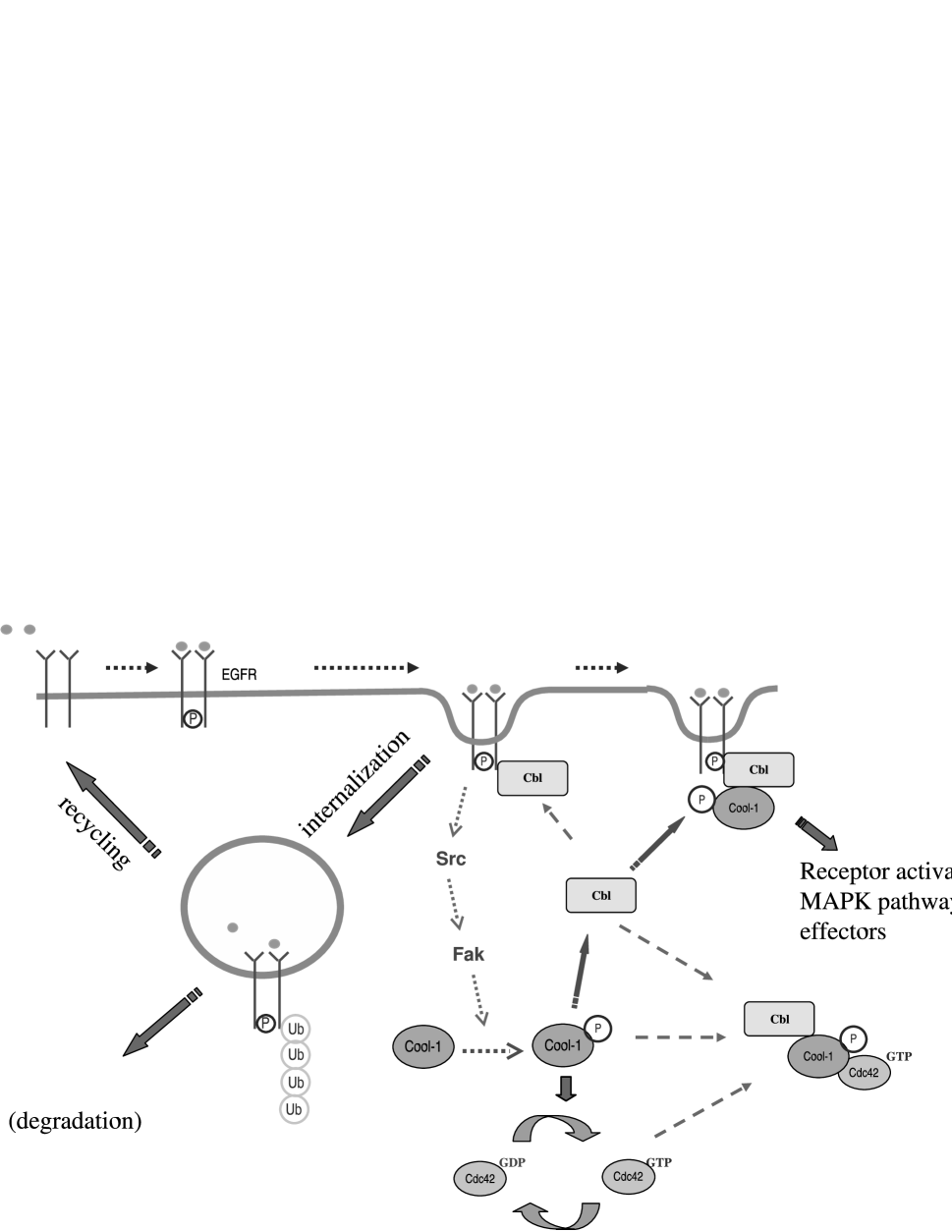
Figure 1: Schematic diagram showing the set of interactions in the model of EGFR signaling, endocytosis and down-regulation (see also qiyulatest ). Phosphatases are not shown.

The goals of this manuscript are to demonstrate how a modeling approach can be used to

• refine the necessary set of interactions in the biological network,

• make predictions on unmeasured components of the system with good precision and

• reduce the prediction uncertainty on components that are difficult to measure directly, by using the methods of optimal experimental design.

II Methods

II.1 Mathematical model, parameter and prediction uncertainties

Before we introduce the algorithms needed to address the design question, we define the model and data in more detail. Our differential equation model for EGFR signaling and down-regulation contains 56 unknown biochemical constants: 53 unknown rate and Michaelis Menten constants (where they can be found, initial estimates were drawn from the literature), and 3 unknown initial conditions which we found useful to vary. The dynamical variables are comprised of 41 separate chemical species, including complexes. The data consist entirely of time series in the form of Western blots. (The data both come from the lab of the co-authors and from the literature, see supplementary information for details.) We have been careful to select data only on NIH-3T3 cells, and in experimental conditions where the cell has been serum-starved prior to EGF stimulation, to prevent activation events not related to the EGFR ligand binding. Most of the time series data are over a period less than a few hours which allows us to ignore transcriptional processes.

Since we have no information on most of the biochemical constants, we must infer them from the data. Therefore we optimize a cost function which measures the discrepancy of simulated data from the real data,

$$C(\theta)=\sum_{\alpha=1}^{D}\sum_{i=1}^{m_{\alpha}}\left(\frac{y_{\alpha}(t_{\alpha i},\theta)-d_{\alpha i}}{\sigma_{\alpha i}}\right)^{2}$$ (1)

where $\alpha$ is an index on the $D$ measured species, $m_{\alpha}$ is the number of time points on species $\alpha$, $y$ is the trajectory of the differential equation model, $\theta$ is a vector of the logarithm of the biochemical constants, $d_{\alpha i}$ is the measured value at time $t_{\alpha i}$ for species $\alpha$ and $\sigma_{\alpha i}$ is the error on the measured value. In other words, we have a standard weighted least squares problem to reduce the discrepancy of the model output to the data by varying $\theta$. (We use the logarithm of the biochemical constants as it allows us to apply an unconstrained optimization method while maintaining the positivity constraint and it removes the discrepancies between biochemical values that have naturally different scales in the problem). As absolute numbers of proteins in the network cannot be accurately measured, data sets measuring activities of proteins are fit up to an arbitrary multiplicative scale factor, which adds parameters to the model not of direct inferential interest (nuisance parameters). Where the relative quantity of a species can be measured (normalized by the level before EGF stimulation for example), the output of the differential equations are similarly scaled by an appropriate common factor.

After the model has been successfully fit to the experimental data, we have a parameter estimate $\hat{\theta}$ which in general will have large covariances, approximated by the inverse of the Fisher information matrix (FIM). The FIM is defined as

$$M = \mathbf{E}[\partial^{2}C/\partial\theta^{2}]$$ (2)

$$= \sum_{\alpha=1}^{D}\sum_{i=1}^{m_{\alpha}}\frac{1}{\sigma_{\alpha i}}\frac{\partial y_{\alpha}(t_{\alpha i},\theta)}{\partial\theta}^{t}\big{|}_{\hat{\theta}}\frac{1}{\sigma_{\alpha i}}\frac{\partial y_{\alpha}(t_{\alpha i},\theta)}{\partial\theta}\big{|}_{\hat{\theta}}$$ (3)

$$= J^{t}J\quad.$$ (4)

where the expectation is over the distribution of errors in the data, which are assumed to be Gaussian. The expression for the FIM above is exact when the model fits perfectly, i.e. at the best fit, the expectation of the residuals is zero, $\mathbf{E}[y_{\alpha}(t_{\alpha i})-d_{i}]=0$. The $i^{th}$ parameter uncertainty is given by the square root of the $i^{th}$ diagonal element of the inverse FIM. $J=\frac{1}{\sigma_{\alpha i}}\partial y_{\alpha}(t_{\alpha i},\theta)/\partial\theta|_{\hat{\theta}}$ is the the sensitivity matrix of residuals with respect to parameters at the best fit and is the analog to the design matrix in a linear regression setting. The design space is the range of species $\alpha$ and of time points $t_{\alpha i}$ for which measurements could be taken. ($\alpha i$ is the row index of $J$.)

We can also make predictions on components of the trajectory (measured or unmeasured), $\hat{y}_{\beta}(t)=y_{\beta}(t,\hat{\theta})$. The variances on these quantities are given by

$$\mbox{Var}(\hat{y}_{\beta}(t))\approx\frac{\partial y_{\beta}(t,\theta)}{\partial\theta}^{t}|_{\hat{\theta}}M^{-1}\frac{\partial y_{\beta}(t,\theta)}{\partial\theta}|_{\hat{\theta}}$$ (5)

The form of Eqn. 5 can be thought of as a combination of the underlying parameter uncertainty, quantified by $M^{-1}$, and the linear response of the system to the parameter uncertainty, quantified by the sensitivities. Note that $M$ is also computed using the sensitivities of the trajectory of the differential equations, which we obtain by implementing the forward sensitivity equations sundials . In practice, $M$ is close to singular if we do not include some prior information on parameter ranges. Therefore we assume a Gaussian prior on the parameters centered on the best fit values and with a standard deviation of $\log(1000)$. (This corresponds to an approximately 1000-fold increase or decrease in the non-logarithmic best fit biochemical values.)

We recognize there can be other sources of uncertainty in predictions, for example if the dynamics of the system are modeled stochastically or if there is model uncertainty that needs to be taken into account. The former is not relevant here as the measurements we fit are not on the single cell level, but rather the average of large populations of cells. The latter is certainly of interest but we choose an approach where model errors are corrected during the fitting and validation process, rather than included a priori in the model definition.

Given the approximate nature of variance estimates derived from the Fisher information matrix and the linearized model response, we supplemented these calculations with a computationally intensive Bayesian Markov Chain Monte Carlo (MCMC) method to compute credible intervals for the predictions we make on the model (see supplementary material). The estimates from the Bayesian MCMC approach are in sufficient agreement with the linearized error anaylsis results that we believe the optimal experimental design algorithms introduced below are justifiably aimed at reducing the approximate uncertainties of Eqn. 5. Using MCMC for error estimates within the framework of the optimal design algorithms would be computationally infeasible.

II.2 Optimal Experimental Design

Optimal experimental design is a technique for deciding what data should be collected from a given experimental system such that quantities we wish to infer from the data can be done so with maximum precision. Typically the network as shown in Fig. 1 has components that can be measured (e.g. total levels of active Cdc42, total levels of surface receptor etc.) and components that are not directly measurable (e.g. levels of the triple complex comprising Cool-1, Cdc42 and Cbl). Therefore we can pose the question of how to minimize the average prediction uncertainty on some unmeasurable component of interest by collecting data on measurable components of the system (we will use the term unmeasurable loosely for the remainder to describe species that are between difficult and impossible to measure by standard methods). This is just one possible design criterion, called V-optimality in the literature; other criteria involve minimizing the total parameter uncertainty in the system (D-optimality), minimizing the uncertainty in the least constrained direction in parameter space (E-optimality) or minimizing the maximum uncertainty in a prediction (G-optimality) Atkinson . Other authors Klingmuller ; Banga ; optimalsamplingtimes have focused on reducing parameter uncertainty but we believe that complex biological models, even with large amounts of precise time series data, have intrinsically large parameter uncertainty kevin1 ; Ryan ; Josh . On the other hand, even with no extra data collection, the uncertainty on unmeasured time trajectories in these biological systems can be surprisingly small despite the large parameter uncertainty Ryan .

By altering the form of the matrix $J$ in Eqn. 4, by measuring different species at different times, we have the possibility of reducing the average variance of $\hat{y}_{\beta}$, which is an integral over time of the quantity defined in Eqn. 5. We discuss the types of design and algorithms that can be used to achieve this.

A distinction must be made between starting designs and sequential designs. A starting design is one in which no data has been collected and the experimenter would like to know what design is best to minimize a given criterion function. Within this category are two subcategories: exact designs and continuous designs. Exact designs refer to the optimal placement of a finite number of design points. As the the design points need to be assigned amongst all the measurable species in the system the optimization problem is of a combinatorial nature. There have been specific algorithms developed for this situation Atkinson which involve choosing some initial design with the required number of points and then randomly modifying it by doing exchanges, additions and deletions. More general global optimization algorithms have been applied to the problem of finding exact designs in differential equation and regression models JonesWang ; globOptDesign .

Continuous designs refer to the selection of a design measure, $\eta$, which is equivalent to a probability density over the design space. The advantage of assuming a continuous design is that the criterion function can then be differentiated with respect to the design measure and tests for optimality can be derived. Asymptotically, for a large number of design points the continuous and exact designs should coincide. For a linear model described by $y=f(t)^{t}\theta+\epsilon$ where $f(t)\in\mathbf{R}^{N}$ and $\epsilon$ is an error term, the FIM is

$$M(\eta)=\int_{\tau}f(t)f(t)^{t}\eta(x)\,dt$$

by definition of the design measure, $\eta$. However, $M$ is a symmetric $N\times N$ matrix made up of a convex combination of the rank one symmetric matrices, $f(t)f(t)^{t}$. Therefore it can be represented by a convex combination of at most $N(N+1)/2$ design points (from Caratheodory’s Theorem) $x_{1},\ldots,x_{N(N+1)/2}$, i.e. as a convex combination of delta function probability measures on those points. In other words even continuous optimal designs for linear models have only a finite number of design support points Silvey . In one of the approaches that follows, we will attempt to find a continuous design by approximating the design measure by a number of finely spaced measurement points with weights associated with each one, and we will see that a near optimal design is in fact only supported on a small subset of those points.

Sequential designs are more relevant to the situation we consider here: experimental data have already been collected and the model has already been fit. Therefore we can get an initial estimate for the parameters in the system and we can evaluate the FIM. Suppose that the current design already has $n$ points and the current FIM is $M_{n}=J_{n}^{t}J_{n}$. The effect of adding the $(n+1)^{th}$ design point (e.g. $y_{\alpha}$ at time point $t_{\alpha i}$) merely adds a single row to $J_{n}$. Therefore the new FIM is the old FIM plus a rank one update:

$$M_{n+1}=J_{n+1}^{t}J_{n+1}=J_{n}^{t}J_{n}+\frac{\partial y_{\alpha}(t_{\alpha i})}{\partial\theta}\big{|}_{\hat{\theta}}\frac{\partial y_{\alpha}(t_{\alpha i})}{\partial\theta}^{t}\big{|}_{\hat{\theta}}\quad.$$

The new inverse FIM is also a sum of terms (by applying the Sherman-Woodbury-Morrison formula VanLoan ): one involving the inverse of the old FIM and the other involving the sensitivity vector at the new point, $\partial y_{\alpha}(t_{\alpha i})/\partial\theta|_{\hat{\theta}}$, so evaluating Eqn. 5 for a large number of proposed measurements is computationally inexpensive.

We take an approach which is a combination of continuous design and sequential design: assume that some initial experiments have already been carried out and we have an FIM for the system. We will then define a cost function $K(\alpha,t_{\alpha i})$ based on the integral of Eqn. 5 and minimize it with respect to $\alpha$ and $t_{\alpha i}$. Initially the minimization looks for the best single data point to reduce the uncertainty (a sequential design method). Once we know for which species the data needs to be collected, we can then place many potential measurements on that species with associated weights and minimize over the weights (to mimic continuous design methods where the set of weights is the approximate design measure).

III Results

III.1 Model refinements

The model was fit to 11 data sets, all Western blot data that describe various signaling, internalization and degradation events that are triggered after receptor activation by ligand, see supplementary information for the full set of fitted time series and description of experiments. As an example of a experimental fit with uncertainties, we show in Fig. 2 the best fit time course and standard deviation for total surface receptor from one of the experiments for which data was included in the model (experiment 1 in supplementary information).

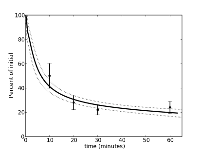
Figure 2: Example of experimental fit and uncertainties around the best fit trajectory (dotted lines) for total surface receptor (in experiment 1 in supplementary information).

During the iterative process of fitting and model refinement we discovered certain interactions and model parameters had to be adjusted to be consistent with the experimentally observed behavior. We briefly summarize these adjustments below.

(1) It appears necessary to incorporate an interaction to allow the triple complex to be dissociated by a dephosphorylation reaction. In particular a reaction was needed whereby Cool-1 within the complex could be inactivated by its own dedicated phosphatase (a possible candidate already present in the system is SHP-2, which has been shown to dephosphorylate the related Sprouty protein shp ). Without this effect, we would not observe the complete deactivation of Cool-1 as it would be “protected” within the triple complex. Additionally, a sensitivity analysis to determine dominant reactions in the model identified phosphatase reactions as important (see supplementary material).

(2) Interestingly, there is an important balance between the level of receptor and Cool-1 in the system to maintain the correct dynamics: if the level of receptor greatly exceeds the Cool-1 level, then the activated receptor will lead indirectly to phosphorylation of Cool-1 which in turn sustains the level of signaling receptor before significant amounts can be endocytosed. It is also essential that the protein level of Cdc42 in the system be sufficiently high, approximately balanced with the Cbl levels as they both come together in the triple complex. If this was not so, the greatly reduced Erk pathway signaling we see in the data set for the Cdc42 knockdown would not be possible to reproduce (supplementary information, experiment 8). Of course, Cdc42 is involved in many other cellular processes, so what is actually important here is the amount available to participate in interactions with Cbl.

(3) The F28L fast cycling (hyperactive) mutant of Cdc42 has the ability to delay endogenous receptor down-regulation for many hours beyond wild type cells (see experiment 5 in the supplementary information). This is only possible if the binding affinity of active Cdc42 to the Cool-1-Cbl complex is strong enough to deplete the levels of the latter and force the forward binding reaction of Cbl to activated Cool-1. This provides a mechanism to sequester more of the Cbl protein (in both the triple complex and the Cool-1-Cbl complex) than would otherwise be possible.

In addition to the above adjustments, we made the following observations relating to the network dynamics and structure.

We find that given these experimental data sets, an endocytosis mechanism which is Cbl dependent and solely acts on activated receptors is completely consistent, although we acknowledge that there is much controversy in the literature as to the dominant endocytosis mechanisms and required regulators. Incorporating a Cbl independent and Cbl dependent mechanism in the same model does not improve the fit. However, given only a Cbl independent endocytosis mechanism, the model would be unable to account for the apparent saturation of the internalization rates for overexpressed receptors (experiments 1-3 in supplementary information) compared to endogenous receptors (experiment 5 in supplementary information). Therefore having a Cbl dependent pathway is convenient in explaining those experimental observations, although any number of proteins, not in the model, could cause saturation in the endocytic pathway.

Despite the apparently earlier activation of Cdc42 than its putative GEF, active Cool-1, (see experiments 10 and 11 in supplementary information) the data still supports a mechanism whereby Cdc42 activation only occurs through Cool-1. The explanation of this effect is that the level of Cool-1 is significantly higher than Cdc42. Then, while only a fraction of Cool-1 is being activated at early times, it is still sufficient to induce substantial activation of Cdc42. This is an example of an apparently contradictory experimental result which only after quantitative modeling is shown still to be consistent with the proposed mechanism. In particular, we found there was no need to invoke another parallel activation mechanism for Cdc42 (through Vav for example) as initially might have been assumed.

It is in the preceding way that the interactions in the system are tuned and modified to describe the observations, and where we get insight into the mechanisms of regulation. As new experimental data are collected, the model may have to be modified again. To decide this, the new data must be matched against predictions from the current model. If the predictions with uncertainties suggest behavior contrary to the observed behavior, we would need to redefine the model.

III.2 Predictions

Once we have a model which reproduces the experimental observations, we would like to make predictions on unmeasured or unmeasurable components of the system. The motivation is twofold. Firstly, if we make a prediction on a currently unmeasured component of the system which is subsequently measured, we have an opportunity to test the validity of our model. Secondly, if we are confident in the model, we may want to test a hypothesis about the role of an unmeasurable component in the system. If that unmeasurable component has large uncertainties, we then need to apply the methods of experimental design to improve the situation. We will discuss these issues in what follows.

III.2.1 Model validation

To first give an example of model validation, consider the qualitative observation in qiyulatest that in stably expressing v-Src cells, in conditions where Cool-1 is overexpressed, ligand-induced receptor internalization is blocked compared to an endogenous Cool-1 control, for at least 60 minutes. The model is adjusted to simulate the conditions of these v-Src cells by making all Src in its active form, switching off Src inactivation and increasing the initial amounts 10-fold to mimic the stable transfection. We then predict the total surface receptor number under the two conditions and assign uncertainties using Eqn. 5. The results are shown in Fig. 3.

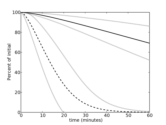
Figure 3: Total surface receptor numbers after EGF stimulation in stably expressing v-Src cells. Endogenous levels of Cool-1 (dashed curve) or overexpressed Cool-1 (solid curve). The dotted lines show the uncertainties in each of the best fit predictions

The qualitative observation of strong inhibition of internalization under conditions of overexpressed Cool-1 is verified by the model. Note that in this case the uncertainties are small enough that we can confidently predict a large difference in the fraction of receptors on the cell surface after 60 minutes under the two conditions. Interestingly, the model also predicts this inhibition is much weaker in cells that are not stably expressing v-Src, essentially because the Cool-1 is not “pre-activated” and endocytosis of significant numbers of receptors can occur before the pool of Cool-1 can become phosphorylated.

III.2.2 Optimal design for the triple complex

Another question of interest is whether the triple complex, which appears to be responsible for sequestering Cbl and blocks receptor down-regulation when Cdc42(F28L) is expressed, also forms in appreciable amounts in wild type cells. We would assume the answer is affirmative, as we observe a reduced downstream mitogenic signal from the receptor under conditions of knockdown of Cool-1 or Cdc42. Since the triple complex is an example of a species that is very difficult to obtain an accurate set of measurements for, we can test a hypothesis about its formation in wild type cells by looking at its predicted time course, Fig. 4.

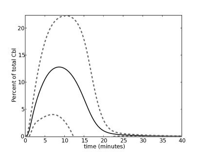
Figure 4: Predictions with uncertainty on the time course of the triple complex consisting of active Cool-1, Cbl and active Cdc42. The quantity plotted is the percentage of total Cbl that is bound in the triple complex.

The relative amount of the triple complex is shown in Fig. 4, where the number of molecules of the triple complex has been scaled relative to the total level of Cbl. Relative levels of complexes and the times of formation/dissociation are more meaningful quantities than absolute numbers of molecules, which are merely rough estimates used to initialize the simulations. The best fit trajectory for the triple complex suggests that at a maximum over 12% of Cbl is sequestered in the complex which represents a significant proportion. However the uncertainty bounds are too large to make this assertion; at the level of the lower bound, less than 4% of Cbl is sequestered at a maximum, and the triple complex dissociates within 15 minutes. This motivates the need for an optimal design approach. We define a criterion which is the average uncertainty in the prediction on the triple complex. We then optimize this quantity using a sequential design approach (therefore we need to perform only line minimizations in the time coordinate for each of the 11 measurable species in the system) and follow up by finding an approximate optimal continuous design on that species. The results of such an analysis are shown in Fig. 5.

             

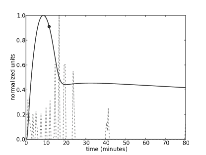
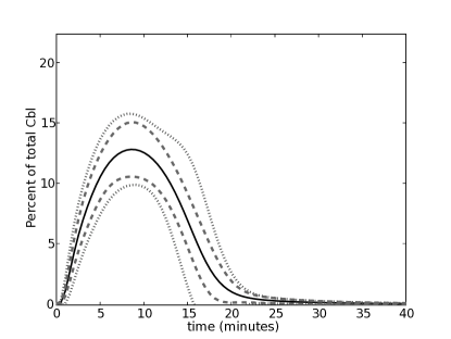
                                    (a)                                                                      (b)                                             

Figure 5: (a) Trajectory of total active Cdc42 (solid line) with single sequential design measurement (marked with a dot) and approximate continuous design weights (dotted line) to reduce the average variance of the prediction on the Cool-1, Cbl, Cdc42 complex. The weights are optimized over 160 uniformly spaced hypothetical measurements placed between 0 and 80 minutes on Cdc42. (b) Shows the reduction in the original uncertainty bounds resulting from the single measurement (dotted line) and the approximate continuous design measurement (dashed line) in (a). Compare with Fig. 4 before the addition of new measurements.

The most striking features of the optimal design results are that

1. a single measurement on total active Cdc42 can significantly reduce the variance we see in the prediction on the triple complex, as in Fig. 5 (b)

2. even though the approximate continuous design allows for 160 hypothetical measurements on the activity of Cdc42, the optimal design weights are concentrated to just a dozen early time points. That is, by just taking a few measurements we can get a design very close to the optimal continuous design for measuring total active Cdc42.

It is worth noting here that these extra measurements have little effect on the parameter uncertainty. In Fig. 6 on the left, we show the eigenvalues of the approximate covariance matrix $M^{-1}$ both before and after the addition of the new data points. On the right is the square root of the diagonal elements of $M^{-1}$, giving the standard deviation in each parameter. As can be seen, the large parameter uncertainties are changed little after the addition of the optimal data points.

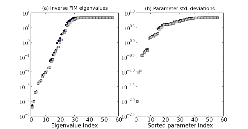
Figure 6: (a) Eigenvalues of the approximate parameter covariance matrix, $M^{-1}$, with (light squares) and without (dark circles) the optimally designed data to reduce the uncertainty of the triple complex trajectory. (b) Individual parameter standard deviations, sorted from smallest to biggest with (light squares) and without (dark circles) the optimally designed data. Note that the cutoff in the spectrum of eigenvalues is due to the prior information assumed on parameters ranges. Even with prior information, 40 of the 60 parameters have uncertainties corresponding to a greater than 20-fold increase or decrease in their non-logarithmic values.

In a sense, the underlying parameter uncertainty defined by $M^{-1}$ in Eqn. 5, although large in some directions, is mostly aligned with directions where the model sensitivity is small. Conversely, if we include hypothetical measurements on the binding and unbinding constants involved in forming the triple complex, we find only a negligibly small decrease in the uncertainty in the prediction of the triple complex (see supplementary information). This is not so surprising when we understand that the uncertainty arises from the uncertainties in components of the system upstream of the triple complex; using parameter measurements alone, almost every rate constant in the system would have to be measured accurately to constrain the prediction Ryan .

III.2.3 New measurements on total active Cdc42

Further measurements were made on total activated Cdc42 in the lab by Western blotting and with no refitting, our model was able to match the new data using a scale factor alone, see Fig. 7. (However, we cannot consider this as a validation of our model, since prior to the inclusion of the new data, the uncertainties on total activated Cdc42 were very large. Any experimental observations within the uncertainty bounds would be consistent with the model.) The uncertainties of the triple complex time course, given the real data and the optimally weighted data, is shown in Fig. 7 (b).

       

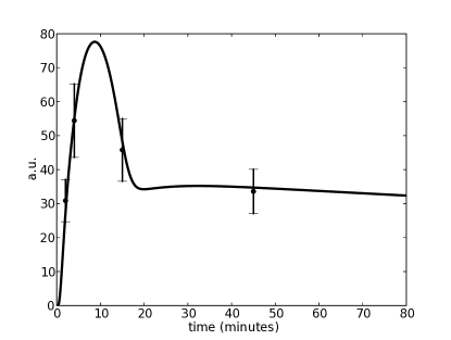
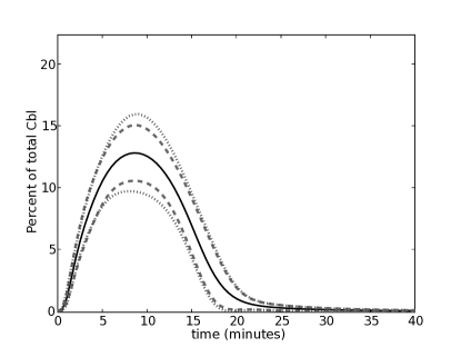
                                (a)                                                                      (b)

Figure 7: (a) Without refitting to the new total active Cdc42 data, our prediction matches the data using only a single multiplicative factor. a.u. = arbitrary units. (b) Reduced uncertainty on the time course of the active Cool, Cbl, and active Cdc42 complex for the optimal set of design points (dashed line) (same as Fig. 5 (b) ) and for the real data (dotted line).

Importantly, given that the measured activities of total Cdc42 were consistent with the trajectory for the optimized set of parameters, the reduction in uncertainty of the triple complex for the real data is comparable to that for the optimally selected data and we can make a firm conclusion that the triple complex does sequester significant amounts of the Cbl protein even in wild type cells after EGF stimulation. Therefore it appears that the complex plays a part under normal conditions in the EGFR homeostasis. (Note that if the new data collected showed a very different time course than in Fig. 7, an additional re-optimization step would need to be performed before we could assess the prediction and uncertainties for the triple complex.)

IV Discussion

We have demonstrated that by quantitatively modeling the dynamics of EGFR signaling and down-regulation in a mammalian cell line, we are led to incorporate interactions and modify existing reactions in order to reproduce the experimental observations. Note that these interactions are not directly tested by experiments, but we can infer them from the existing data. This refinement of an existing model of interactions and parameters is one important aspect of the modeling effort and gives insight into the underlying dynamics. Of course, we recognize that the model as it stands will only explain the behaviors observed in the data sets we have chosen. The addition of new experiments that test for receptor signaling from early endosomes endosomalSig , alternative endocytic mechanisms difiore , autocrine signaling autocrine1 ; autocrine2 or the interactions between members of the erb-B family erbBfamily , for example, will require appropriate extensions of the mathematical model.

The second part of the process is to make predictions on the unmeasured or unmeasurable species of the system, assuming that the model has been suitably refined. We suggest that for testable predictions to be made, uncertainty estimates need to be attached to them kevin1 . In some cases the prediction uncertainties are rather small, despite large parameter uncertainty. On the other hand, if some predictions show large uncertainty, and involve species that are not directly measurable, we may then define a suitable design criterion and suggest new experimental measurements that need to be taken to reduce that uncertainty. The results of such an analysis are promising, in that we find a rather small number of measurements (realistic to perform with standard molecular biology techniques) need be taken to begin to make predictions with good precision. Given such measurements on the EGFR system, we see that the triple complex of active Cool-1, Cbl and active Cdc42 does indeed form in appreciable quantities in wild type cells and we also get an estimate for the time of formation and dissociation.

More generally, we believe that experimental design for reducing prediction uncertainties can play an important role in the iterative process of model refinement and validation and can be used in the testing of biological hypotheses.

References

- (1) Feng, Q., Baird, D., Peng, X., Wang, J., Ly, T., Guan, J-L., and Cerione, R. A. ‘Cool-1 functions as an essential regulatory node for egf receptor- and src-mediated cell growth’, Nature Cell Biology, 2006, DOI: 10.1038/ncb1453.
- (2) Wu, W. J., Tu, S., and Cerione, R. A. ‘Activated cdc42 sequesters c-cbl and prevents egf receptor degradation’, Cell, 2003, 114, pp. 715–725.
- (3) Carpenter, G. ‘The egf receptor : a nexus for trafficking and signaling’, BioEssays, 2000, 22, pp. 697–707.
- (4) Wells, A., Welsh, J. B., Lazar, C. S., Wiley, H. S., Gill, G. N., and Rosenfeld, M. G. ‘Ligand-induced transformation by a non-internalizing epidermal growth factor receptor’, Science, 1990, 247, pp. 962–964.
- (5) Hirsch, F. R., Varella-Garcia, M., Bunn Jr., P. A., Maria, M. V. Di, Veve, R., Bremmes, R. M., Baron, A. E., Zeng, C., and Franklin, W. A. ‘Epidermal growth factor receptor in non-small-cell lung carcinomas: correlation between gene copy number and protein expression and impact on prognosis’, J. Clin. Oncol., 2003, 20, pp. 3798–3807.
- (6) DiGiovanna, M. P., Stern, D. F., Edgerton, S. M., Whalen, S. G., II, D. Moore, and Thor, A. D. ‘Relationship of epidermal growth factor receptor expression to erbb-2 signaling activity and prognosis in breast cancer patients’, Journal of Clinical Oncology, 2005, 23, pp. 1152–1160.
- (7) Wong, E. S. M., Fong, C. W., Lim, J., Y, P., Low, B. C., Langdon, W. Y., and Guy, G. R. ‘Sprouty2 attenuates epidermal growth factor receptor ubiquitylation and endocytosis, and consequently enhances ras/erk signalling’, The EMBO Journal, 2002, 21, pp. 4796–4808.
- (8) Ettenberg, S. A., Magnifico, A., Cuello, M., Nau, M. M., Rubinstein, Y. R., Yarden, Y., Weissman, A. M., and Lipkowitz, S. ‘Cbl-b-dependent coordinated degradation of the epidermal growth factor receptor signaling complex’, J. Biol. Chem., 2001, 276, pp. 27677–27684.
- (9) Grovdal, L. M., Stang, E., Sorkin, A., and Madshus, I. H. ‘Direct interaction of cbl with ptyr 1045 of the egf receptor (egfr) is required to sort the egfr to lysosomes for degradation’, Experimental Cell Research, 2004, 300, pp. 388–395.
- (10) Levkowitz, G., Waterman, H., Ettenberg, S. A., Katz, M., Tsygankov, A. Y., Alroy, I., Lavi, S., Iwai, K., Reiss, Y., Ciechanover, A., Lipkowitz, S., and Yarden, Y. ‘Ubiquitin ligase activity and tyrosine phosphorylation underlie suppression of growth factor signaling by c-cbl/sli-1’, Molecular Cell, 1999, 4, pp. 1029–1040.
- (11) Duan, L., Miura, Y., Dimri, M., Majumder, B., Dodge, I. L., Reddi, A. L., Ghosh, A., Fernandes, N., Zhou, P., Mullane-Robinson, K., Rao, N., Donoghue, S., Rogers, R. A., Bowtell, D., Naramura, M., Gu, H., Band, V., and Band, H. ‘Cbl-mediated ubiquitinylation is required for lysosomal sorting of epidermal growth factor receptor but is dispensable for endocytosis’, J. Biol. Chem., 2003, 278, pp. 28950–28960.
- (12) Huang, F. and Sorkin, A. ‘Growth factor receptor binding protein 2-mediated recruitment of the ring domain of cbl to the epidermal growth factor receptor is essential and sufficient to support receptor endocytosis’, Molecular Biology of the Cell, 2005, 16, pp. 1268–1281.
- (13) Jiang, X. and Sorkin, A. ‘Epidermal growth factor receptor internalization through clathrin-coated pits requires cbl ring finger and proline-rich domains but not receptor polyubiquitylation’, Traffic, 2003, 4.
- (14) Mosesson, Y., Shtiegman, K., Katz, M., Zwang, Y., Vereb, G., Szollosi, J., and Yarden, Y. ‘Endocytosis of receptor tyrosine kinases is driven by monoubiquitylation, not polyubiquitylation’, J. Biol. Chem., 2003, 278, pp. 21323–21326.
- (15) Sigismund, S., Woelk, T., Puri, C., Maspero, E., Tacchetti, C., Transidico, P., Fiore, P. P Di, and Polo, S. ‘Clathrin-independent endocytosis of ubiquitinated cargos’, PNAS, 2005, 102, pp. 2760–2765.
- (16) Szymkiewicz, I., Kowanetz, K., Soubeyran, P., Dinarina, A., Lipkowitz, S., and Dikic, I. ‘Cin85 participates in cbl-b-mediated downregulation of receptor tyrosine kinases’, J. Biol. Chem., 2002, 277, pp. 39666–39672.
- (17) Schoeberl, B., Eichler-Jonsson, C., Gilles, E. D., and Muller, G. ‘Computational modeling of the dynamics of the map kinase cascade activated by surface and internalized egf receptors’, Nature Biotechnology, 2002, 20, pp. 370–375.
- (18) Kholodenko, B. N., Demin, O. V., Moehren, G., and Hoek, J. B. ‘Quantification of short term signaling by the epidermal growth factor receptor’, J. Biol. Chem., 1999, 274, pp. 30169–30181.
- (19) Resat, H., Ewald, J. A., Dixon, D. A., and Wiley, H. S. ‘An integrated model of epidermal growth factor receptor trafficking and signal transduction’, Biophys. J., 2003, 85, pp. 730–743.
- (20) Blinov, M. L., Faeder, J. R., Goldstein, B., and Hlavacek, W. S. ‘A network model of early events in epidermal growth factor receptor signaling that accounts for combinatorial complexity’, BioSystems, 2006, 83, pp. 136–151.
- (21) Serban, R. and Hindmarsh, A. C., ‘Cvodes: An ode solver with sensitivity analysis capabilities’, LLNL technical report UCRL-MA-148813, Lawrence Livermore National Labs, 2002.
- (22) Atkinson, A. C. and Donev, A. N., Optimum Experimental Design. New York: Oxford University Press, first ed., 1992.
- (23) Faller, D., Klingmuller, U., and Timmer, J. ‘Optimal experimental design in systems biology’, Simulation, 2003, 79, p. 717.
- (24) Kutalik, Z., Cho, K-H., and Wolkenhauer, O. ‘Optimal sampling time selection for parameter estimation in dynamic pathway modelling’, BioSystems, 2004, 75, pp. 43–55.
- (25) Rodriguez-Fernandez, M., Mendes, P., and Banga, J. R. ‘A hybrid approach for efficient and robust parameter estimation in biochemical pathways’, BioSystems, 2006, 83, pp. 248–265.
- (26) Brown, K.S. and Sethna, J.P. ‘Statistical mechanics approaches to models with many poorly known parameters’, Phys. Rev. E., 2003, 68, p. 021904.
- (27) Gutenkunst, R.N., Waterfall, J.J., Casey, F.P., Brown, K.S., Myers, C.R., and Sethna, J.P., ‘Sloppy systems biology: tight predictions without tight parameters’, 2006. Submitted.
- (28) Waterfall, J.J., Casey, F.P., Gutenkunst, R.N., Brown, K.S., Myers, C.R., Brouwer, P.W., V.Elser, and Sethna, J.P., ‘The sloppy model universality class and the vandermonde matrix’, 2006. Accepted.
- (29) Boer, E. P. J. and Hendrix, E. M. T. ‘Global optimization problems in optimal design experiments in regression models’, Journal of Global Optimization, 2000, 18, pp. 385–398.
- (30) Jones, B. and Wang, J. ‘Constructing optimal designs for fitting pharmacokinetic models’, Statistics and Computing, 1999, 9, pp. 209–218.
- (31) Silvey, S. D., Optimal Design: an introduction to the theory for parameter estimation. London: Chapman and Hall, first ed., 1980.
- (32) Golub, G.H. and Loan, C.F. Van, Matrix Computations. Baltimore: The Johns Hopkins University Press, third ed., 1996.
- (33) Hanafusa, H., Torii, S., Yasunaga, T., Matsumoto, K., and Nishida, E. ‘Shp2, an sh2-containing protein-tyrosine phosphatase, positively regulates receptor tyrosine kinase signaling by dephosphorylating and inactivating the inhibitor sprouty’, J. Biol. Chem., 2004, 279, pp. 22992–22995.
- (34) Burke, P., Schooler, K., and Wiley, H. S. ‘Regulation of epidermal growth factor receptor signaling by endocytosis and intracellular trafficking’, Molecular Biology of the Cell, 2001, 12, pp. 1897–1910.
- (35) Shvartsman, S. Y., Hagan, M. P., Yacoub, A., Dent, P., Wiley, H. S., and Lauffenburger, D. A. ‘Autocrine loops with positive feedback enable context-dependent cell signaling’, Am J Physiol Cell Physiol, 2002, 282, pp. C545–C559.
- (36) Shvartsman, S. Y., Wiley, H. S., Deen, W. M., and Lauffenburger, D. A. ‘Spatial range of autocrine signaling: Modeling and computational analysis’, Biophysical Journal, 2001, 81, pp. 1854–1867.
- (37) Hendriks, B. S., Cook, J., Burke, J. M., Beusmans, J. M., Lauffenburger, D. A., and de Graaf, D. ‘Computational modelling of erbb family phosphorylation dynamics in response to transforming growth factor alpha and heregulin indicates spatial compartmentation of phosphatase activity’, IEE Proc.-Syst. Biol., 2006, 1, pp. 22–33.