Quartet consistency count method for reconstructing phylogenetic trees

Abstract.

Among the distance based algorithms in phylogenetic tree reconstruction, the neighbor-joining algorithm has been a widely used and effective method. We propose a new algorithm which counts the number of consistent quartets for cherry picking with tie breaking. We show that the success rate of the new algorithm is almost equal to that of neighbor-joining. This gives an explanation of the qualitative nature of neighbor-joining and that of dissimilarity maps from DNA sequence data. Moreover, the new algorithm always reconstructs correct trees from quartet consistent dissimilarity maps.

1. Introduction

The neighbor-joining algorithm is widely used among all distance based methods for phylogenetic tree reconstruction. In spite of its simplicity neighbor-joining has become a de facto standard and continued to surface as an effective candidate method for constructing large phylogenies. There have been many studies relating to neighbor-joining in many aspects (Atteson,, 1999; Bryant,, 2005; Levy et al.,, 2006; Mihaescu et al.,, 2006). Questions like how, when, and why neighbor-joining works, have been the main issues in the empirical and theoretical studies of phylogenetic tree constructions.

We propose a new algorithm, Quartet Consistency Count abbreviated to QCC, which gives a partial answer for these questions. How does the QCC algorithm work? The QCC algorithm replaces the cherry picking criterion in neighbor-joining with a new one, the $QC$-criterion in Theorem 3, which is to find a pair having maximum quartet consistency counts.

The observation is that there are many irrelevant pairwise distances estimated from DNA sequence data which might reconstruct wrong trees. The noises or errors from a dissimilarity map are accumulated to pick irrelevant cherries in neighbor-joining. However quartet consistency determines how four species are partitioned into two pairs, and its structure is well preserved in the empirical DNA sequence data. It is reasonable to consider quartet consistency rather than adding the lengths of related edges as neighbor-joining.

When does the $QC$-criterion always reconstruct a correct tree? Atteson proved in (Atteson,, 1999) that neighbor-joining always reconstructs a correct tree when $l_{\infty}$ radius is $\frac{1}{2}$. The $QC$-criterion also has the same $l_{\infty}$ radius which is proved in Corollary 7. Unfortunately, very small percentage of DNA sequence data does satisfy the $l_{\infty}$ radius condition. However the $QC$-criterion always works under the condition when all quartets are consistent, which is proved in Theorem 6. It is estimated that the quartet consistency rate is relatively high and strongly related with the success rate of neighbor-joining.

The success rate of QCC is remarkably similar to that of neighbor-joining even though the tree topologies they generate are quite different (see Figure 2). Nevertheless QCC takes a quite different path in constructing trees compared to neighbor-joining. A sample data analysis in Figure 3 shows that the rate of picking identical cherries in order is less than 65% even though the two algorithms generate the same tree topologies.

Why do neighbor-joining and QCC work? This question is hard to answer. On the other hand we have seen that the success rates of neighbor-joining and QCC are almost same. Since the success of QCC is due to quartet consistency, it is reasonable to say that neighbor-joining reflects the quartet structure well. The QCC algorithm gives an explanation of the qualitative nature of neighbor-joining and that of dissimilarity maps from DNA sequence data.

2. Quartet consistency and the $QC$-criterion

Recall that a dissimilarity map on $[n]:=\{1,2,\dotsc,n\}$ is a function $d\colon[n]\times[n]\to\mathbb{R}$ such that $d(i,i)=0$ and $d(i,j)=d(j,i)\geq 0$. A dissimilarity map $d$ is called a metric on $[n]$ if the triangle inequality holds: $d(i,j)\leq d(i,k)+d(k,j)$ for all $i,j,k\in[n]$. A metric $d$ is a tree metric if there exists a tree $T$ with $n$ leaves, labeled by $[n]$, and a non-negative length for each edge of $T$, such that the length of the unique path from leaf $x$ to leaf $y$ equals $d(x,y)$ for all $x,y\in[n]$. We sometimes write $d_{T}$ for the tree metric $d$ which is derived from the tree $T$.

Given four leaves $i,j,k,l$ in a tree $T$, we say that $(ij;kl)$ is a quartet if the path from $i$ to $j$ has no common edge to the path from $k$ to $l$. In terms of the tree metric $d_{T}$, it is equivalent to the following four point condition (Buneman,, 1971):

$$d_{T}(i,j)+d_{T}(k,l)\leq d_{T}(i,k)+d_{T}(j,l)=d_{T}(i,l)+d_{T}(j,k).$$ (1)

We define a cherry of a tree by a pair of leaves which are both adjacent to the same (internal) node. This definition of cherry can be reinterpreted as follows: The pair $\{i,j\}$ is a cherry if and only if $(ij;kl)$ is a quartet for any pair of leaves $\{k,l\}\subset[n]\setminus\{i,j\}$. In other words, a cherry of a tree is a pair of leaves which defines maximum quartets combining with all other pairs, the number is always $\binom{n-2}{2}$.

Let $d$ be a dissimilarity map on $[n]$. For any $i,j,k,l\in[n]$ we set

$$w(ij;kl):=\tfrac{1}{4}\bigl{[}d(i,k)+d(j,l)+d(i,l)+d(j,k)-2[d(i,j)+d(k,l)]\bigr{]}.$$

In particular, the function $w$ provides a natural weight for quartets, when $d$ is a tree metric, that is, the length of the path which connects the path between $i$ and $j$ with the path between $k$ and $l$.

The neighbor-joining algorithm makes use of the following cherry picking theorem (Saitou and Nei,, 1987) by peeling off cherries to recursively build a tree.

Theorem 1.

If $d$ is a tree metric on $[n]$, then any pair of leaves that maximizes $Z_{d}(i,j)=\sum_{\{k,l\}\subset[n]\setminus\{i,j\}}w(ij;kl)$ is a cherry in the tree.

An equivalent, but computationally superior, formulation is the following $Q$-criterion (Studier and Keppler,, 1988), which is the unique selection criterion in some sense (Bryant,, 2005).

Corollary 2.

If $d$ is a tree metric on $[n]$, then any pair of leaves that minimizes $Q_{d}(i,j)=(n-2)d(i,j)-\sum_{k\neq i}d(i,k)-\sum_{k\neq j}d(j,k)$ is a cherry in the tree.

We now introduce the notion of quartet consistency and then propose a new criterion called the $QC$-criterion which counts the number of consistent quartets to determine the cherries.

Definition.

A dissimilarity map $d$ is quartet consistent with a tree $T$ if

$$d(i,j)+d(k,l)\leq\min\{d(i,k)+d(j,l),d(i,l)+d(j,k)\}$$ (2)

for all quartets $(ij;kl)$ in $T$. Note that any tree metric $d_{T}$ is quartet consistent with $T$ since $d_{T}$ satisfies the four point condition (1).

Remark.

In terms of the weight function $w$, the quartet consistency condition (2) is equivalent to $w(ij;kl)\geq\max\{w(ik;jl),w(il;jk)\}$ which is used in (Mihaescu et al.,, 2006, Definition 8).

Theorem 3.

If $d$ is a tree metric on $[n]$, then any pair of leaves that maximizes

$$QC_{d}(i,j) :=\text{the number of pairs $\{k,l\}\subset[n]\setminus\{i,j\}$ such that}$$

$$\phantom{:=}\qquad d(i,j)+d(k,l)\leq\min\{d(i,k)+d(j,l),d(i,l)+d(j,k)\}$$

is a cherry in the tree.

Proof.

Since $d$ is a tree metric, the four point condition (1) implies that $QC_{d}(i,j)$ equals the number of pairs $\{k,l\}\subset[n]\setminus\{i,j\}$ such that $(ij;kl)$ is a quartet, which becomes the maximum number $\binom{n-2}{2}$ if and only if $\{i,j\}$ is a cherry. ∎

The following theorem has been a widely used justification for the observed success of neighbor-joining.

Theorem 4 (Atteson (Atteson,, 1999)).

Neighbor-joining has $l_{\infty}$ radius $\frac{1}{2}$.

This implies that neighbor-joining always reconstruct a correct tree if the distance estimates are at most half the minimal edge length of the tree away from their true value. Two conditions are introduced in (Mihaescu et al.,, 2006) to explain why neighbor-joining is useful in practice. One is quartet consistent and the other is quartet additive which appears to be rather technical. It is also verified that Atteson’s theorem is a special case of the following theorem (Mihaescu et al.,, 2006, Theorem 17).

Theorem 5.

If $d$ is quartet consistent and quartet additive with a tree $T$, then neighbor-joining applied to $d$ will construct a tree with same topology as $T$.

Atteson’s condition is sufficient to satisfy the quartet consistent and quartet additive condistions. Since these two conditions are not always satisfied, the success rate of reconstructing a correct tree by neighbor-joining is limited. In practical computation, however, the pairwise distances are estimated from noisy data, and consequently, the resulting dissimilarity map is very unlikely to be a tree metric. The dissimilarity map by estimating distances from DNA sequence data does not satisfy the quartet consistency and quartet additive conditions in most cases even when neighbor-joining is successful. In practical sense, it is not fully understood why neighbor-joining is successful.

We state the consistency theorem for the $QC$-criterion. It says that the $QC$-criterion for cherry picking with the same reduction step as neighbor-joining always reconstruct a correct tree whenever a dissimilarity map is quartet consistent.

Theorem 6.

If a dissimilarity map $d$ is quartet consistent with a tree $T$, then the $QC$-criterion for cherry picking with the reduction step of neighbor-joining applied to $d$ will construct a tree with the same topology as $T$.

Proof.

Since $d$ is quartet consistent with $T$, $QC_{d}(i,j)$ is greater or equal to the number of pairs $\{k,l\}\subset[n]\setminus\{i,j\}$ such that $(ij;kl)$ is a quartet, which becomes the maximum number $\binom{n-2}{2}$ when $\{i,j\}$ is a cherry in $T$. Therefore, the $QC$-criterion always picks a cherry if $d$ is quartet consistent with $T$. It suffices to show that the quartet consistency condition is preserved in the reduction step of neighbor-joining.

Suppose that $\{i,j\}$ is a cherry picked in the previous step. The reduction step of neighbor-joining constructs the reduced tree $\widetilde{T}$ by removing the two leaves $i,j$ and adding a new one $i_{*}$. The dissimilarity map is also modified by the equation $d(i_{*},k)=\frac{1}{2}\bigl{[}d(i,k)+d(j,k)-d(i,j)\bigr{]}$ for all $k\in[n]\setminus\{i,j\}$. We will show that the modified dissimilarity map is quartet consistent with $\widetilde{T}$. Note that $(i_{*}k;lm)$ is a quartet in $\widetilde{T}$ if and only if $(ik;lm)$ and $(jk;lm)$ are both quartets in $T$.

Suppose $(i_{*}k;lm)$ is a quartet in $\widetilde{T}$, then we have

$$d(i,k)+d(l,m)\leq\min\bigl{\{}d(i,l)+d(k,m),d(i,m)+d(k,l)\bigr{\}},$$

$$d(j,k)+d(l,m)\leq\min\bigl{\{}d(j,l)+d(k,m),d(j,m)+d(k,l)\bigr{\}},$$

since $d$ is quartet consistent with $T$. Combining these two inequalities, we get

$$d(i,k)+d(j,k)+2d(l,m)$$

$$\qquad\leq\min\{d(i,l)+d(j,l)+2d(k,m),d(i,m)+d(j,m)+2d(k,l)\}.$$

Therefore

$$d(i_{*},k)+d(l,m)=\tfrac{1}{2}\bigl{[}d(i,k)+d(j,k)+2d(l,m)-d(i,j)\bigr{]}$$

$$\quad\leq\min\bigl{\{}\tfrac{1}{2}[d(i,l)+d(j,l)-d(i,j)]+d(k,m),\tfrac{1}{2}[d(i,m)+d(j,m)-d(i,j)]+d(k,l)\bigr{\}}$$

$$\quad=\min\{d(i_{*},l)+d(k,m),d(i_{*},m)+d(k,l)\}.\qed$$

We can also prove that the $QC$-criterion has $l_{\infty}$ radius $\frac{1}{2}$. This means, like neighbor-joining, if the distance estimates are at most half the minimal edge length of the tree away from their true values then the $QC$-criterion will reconstruct a correct tree. It was proved in (Mihaescu et al.,, 2006, Corollary 20) that the $l_{\infty}$ radius $\frac{1}{2}$ condition implies the quartet consistent and quartet additive conditions. We would like to include a short proof of it to make this paper self-contained.

Corollary 7.

The $QC$-criterion has $l_{\infty}$ radius $\frac{1}{2}$.

Proof.

Suppose that distance estimates are at most half of the minimal edge length of the tree. Then it is quartet consistent with it. Since $\min\bigl{\{}d(i,k)+d(j,l),d(i,l)+d(j,k)\bigr{\}}-\bigl{[}d(i,j)+d(k,l)\bigr{]}$ is less than four times of maximum noises minus two times of length of connecting edge associated with the quartet $(ij,kl)$, if maximum error is less than half of the minimal edge length, the quartet structure is consistent with the tree. ∎

Unlike neighbor-joining, the selection criterion $QC$ is not distance linear (Bryant,, 2005). It rather depends on how a dissimilarity map preserves the quartet structures of a given tree.

Remark.

In (Mihaescu et al.,, 2006, Example 11), they constructed a quartet consistent metric on an eight leaves tree which cannot be reconstructed by neighbor-joining. By Theorem 6, $QC$-criterion will reconstruct the correct tree.

3. Performance of the quartet consistency count algorithm

The Quartet Consistency Count algorithm consists of two steps, one is the cherry picking step and the other is the reduction step. It adopts the $QC$-criterion instead of the $Q$-criterion of neighbor-joining for the cherry picking step, but the same algorithm for the reduction step as neighbor-joining.

We sometimes get different tree topologies for one dissimilarity map if the $QC$-criterion is used solely in the cherry picking step. This happens when there are more than one pair having the same quartet consistency count. In this case the order of picking cherries depends on the order of leaves in the input data, and the resulting tree might have different topologies. To overcome the defect a tie-breaking routine is required in the QCC algorithm.

We have tested several tie breaking methods, one of which gives a penalty for the bad case when the inequality $d(i,j)+d(k,l)>\max\{d(i,k)+d(j,l),d(i,l)+d(j,k)\}$ happens, and another one minimizing the sum of errors, $|d(i,k)+d(j,l)-d(i,l)-d(j,k)|$. Most of all, minimizing the value $Q_{d}(i,j)$ in Corollary 2 gave a better success rate, and it was adopted for the tie breaking routine in the QCC algorithm as follows:

 Quartet Consistency Count Algorithm  Input: A dissimilarity map $d$ on the set $[n]$

Output: A phylogenetic tree $T$ whose tree metric $d_{T}$ is close to $d$

Cherry picking step: Find a pair $\{i,j\}$ having the maximum $QC_{d}(i,j)$ count. If there are more than one such pair, choose a pair having the minimum $Q_{d}(i,j)$ value among them.

Reduction step: Remove $\{i,j\}$ from the tree, thereby creating a new leaf $i_{*}$. For each leaf $k$ among the remaining $n-2$ leaves, set $d(i_{*},k)=\frac{1}{2}[d(i,k)+d(j,k)-d(i,j)]$. Return to the cherry picking step until there are no more leaves to collapse.  

Success rates of QCC and neighbor-joining

The success rate of QCC is discussed in the perspective of neighbor-joining. We tested QCC with simulated data on the two parameter family of trees described in (Saitou and Nei,, 1987). We simulated 1,000 data sets on each of the nine tree shapes, $T_{0}^{n}$, $T_{1}^{n}$, and $T_{2}^{n}$ when the number of leaves $n=8$, $12$, and $16$ (see Figure 1) at the three edge length ratios, $a/b=0.01/0.04$, $0.02/0.13$, $0.03/0.34$ for $T_{0}$, and $a/b=0.01/0.07$, $0.02/0.19$, $0.03/0.42$ for $T_{1}$ and $T_{2}$. This was repeated three times for sequences of length 500, 1000, and 2000 bp. The Juke-Cantor distance method for GTR model was used to get pairwise distances from the simulated DNA sequence data generated by Seq-Gen (Rambaut and Grassly,, 1997).

Figure 1. Nine tree shapes $T_{0}^{n}$, $T_{1}^{n}$, and $T_{2}^{n}$ for $n=8$, $12$, and $16$

Tabel 1 shows the success rate of QCC compared with neighbor-joining. The numbers inside parentheses are the differences between the success rate of QCC and that of neighbor-joining, positive (resp. negative) numbers represent that the success rate of QCC is better (resp. worse) than that of neighbor-joining. It is remarkable that the success rates of the two algorithms are almost same, and that the differences are independent of the tree shapes and the bp lengths of simulated DNA sequence data.

bp	500			1000			2000
$a/b$	$\frac{0.01}{0.04}$	$\frac{0.02}{0.13}$	$\frac{0.03}{0.34}$	$\frac{0.01}{0.04}$	$\frac{0.02}{0.13}$	$\frac{0.03}{0.34}$	$\frac{0.01}{0.04}$	$\frac{0.02}{0.13}$	$\frac{0.03}{0.34}$
$T_{0}^{8}$	68.4	50.7	10.9	91.6	82.8	26.3	99.4	96.9	56.5
	(-0.2)	(-0.3)	(-0.3)	(0.0)	(0.0)	(0.7)	(0.0)	(0.0)	(-0.8)
$T_{0}^{12}$	63.7	44.5	04.2	93.7	85.0	21.0	99.9	99.0	59.1
	(0.1)	(0.1)	(-0.2)	(-0.1)	(-0.7)	(-0.3)	(0.0)	(-0.5)	(-0.3)
$T_{0}^{16}$	39.0	20.3	00.2	83.9	65.2	05.4	99.3	96.0	35.1
	(1.6)	(-0.2)	(-0.1)	(-0.2)	(-0.5)	(0.5)	(0.0)	(-0.9)	(-1.1)
$a/b$	$\frac{0.01}{0.07}$	$\frac{0.02}{0.19}$	$\frac{0.03}{0.42}$	$\frac{0.01}{0.07}$	$\frac{0.02}{0.19}$	$\frac{0.03}{0.42}$	$\frac{0.01}{0.07}$	$\frac{0.02}{0.19}$	$\frac{0.03}{0.42}$
$T_{1}^{8}$	72.5	55.9	10.8	95.4	86.7	32.6	99.9	98.7	65.8
	(0.0)	(-0.3)	(-0.6)	(-0.1)	(-0.2)	(0.1)	(0.0)	(0.0)	(0.1)
$T_{1}^{12}$	59.9	44.0	03.0	93.5	81.3	24.3	99.7	99.0	65.1
	(0.2)	(0.2)	(0.6)	(0.1)	(0.0)	(0.0)	(0.0)	(0.0)	(0.3)
$T_{1}^{16}$	51.0	32.3	01.8	92.0	80.7	15.0	99.6	98.6	55.2
	(0.6)	(0.3)	(-0.4)	(0.5)	(0.4)	(-0.1)	(0.0)	(-0.1)	(0.9)
$a/b$	$\frac{0.01}{0.07}$	$\frac{0.02}{0.19}$	$\frac{0.03}{0.42}$	$\frac{0.01}{0.07}$	$\frac{0.02}{0.19}$	$\frac{0.03}{0.42}$	$\frac{0.01}{0.07}$	$\frac{0.02}{0.19}$	$\frac{0.03}{0.42}$
$T_{2}^{8}$	81.5	68.2	19.0	96.4	91.3	44.2	99.9	98.6	70.0
	(-0.1)	(0.0)	(0.4)	(0.0)	(-0.1)	(-0.4)	(0.0)	(0.0)	(-0.1)
$T_{2}^{12}$	69.0	55.8	04.3	96.6	89.7	26.4	99.8	99.5	60.8
	(-0.5)	(0.4)	(0.3)	(0.0)	(-0.3)	(-1.1)	(0.0)	(0.0)	(0.1)
$T_{2}^{16}$	64.7	47.3	02.2	95.5	87.2	17.9	99.9	99.3	61.0
	(0.0)	(-0.2)	(0.0)	(0.0)	(0.3)	(2.5)	(0.0)	(-0.1)	(-0.4)

Table 1. Success rate of QCC compared with neighbor-joining: The values denote the success rate of neighbor-joining in percentage, and the numbers inside parentheses represent the difference of success rates of QCC compared with neighbor-joining.

Figure 2 shows an interesting fact that the differences do not vary even if the tree topologies generated by the two algorithms are quite different. Note that the difference rate is still quite small when the rate of generating the same tree topologies is around 30%.

Figure 2. Differences of the success rates of neighbor-joining and QCC according to the rate of generating the same tree topologies

Independent cherry picking order

Even success rates of QCC and neighbor-joining are almost same to each other, the paths of picking cherries in order are quite different. We investigated the percentage of picking identical cherries in order out of 1000 data sets for each 81 different trees. It is interesting to see in Figure 3 that the identical percentage is not so high even QCC and neighbor-joining generate the same tree topologies. When the rate of generating the same tree topologies is more than 95%, the identical percentage does not exceed 65% in the simulated data sets. It indicates that the QCC algorithm takes quite different paths of picking cherries compared to neighbor-joining.

Figure 3. The percentage of picking identical cherries in order according to the rate of generating the same tree topologies

Quartet consistency rate and neighbor-joining

Quartet consistency rate of a dissimilarity map is the percentage of four leaves satisfying the quartet consistency condition (2) with a given tree $T$ over all possible quartets in $T$. The QCC algorithm heavily depends on this rate, for instance, it recovers a correct tree when the rate is 100% by Theorem 6.

We investigated in Figure 4 that the correlation of quartet consistency rate with respect to the success rate of neighbor-joining. The correlation coefficient was computed as 0.8736. The graph shows that the success rate of neighbor-joining near 100% is almost same as quartet consistency, as we expected, since the success rates of QCC and neighbor-joining are almost same. Quartet consistency rates also increase as bp lengths increase. The dashed line in the graph, denoted by $T^{8}_{0}$ (resp. $T^{16}_{0}$) connects the three points representing the success rates of neighbor-joining for the tree $T^{8}_{0}$ (resp. $T^{16}_{0}$) with the ratio $a/b=0.01/0.04$ when the bp lengths are 500, 1000, and 2000.

Figure 4. Quartet consistency rate with respect to the success rate of neighbor-joining

4. Discussion

Quartet based methods

There are many quartet based methods in reconstructing the phylogenetic trees. Several methods were proposed in (Bryant and Steel,, 2001) to construct the optimal trees which agree with the largest number of quartets or the maximum weight set of quartets. The general problems are known to be NP-hard. The implemented algorithms, Quartet-Cleaning and $Q^{*}$, have quite different nature statistically compared to neighbor-joining (John et al.,, 2003). The QCC algorithm is quite different to the well-known quartet based methods derived from quartet puzzling problem, it is shown to be close to neighbor-joining.

$QC$-criterion without tie-breaking

The cherry picking step in the QCC algorithm requires a tie-breaking routine to avoid the dependency of the order of the leaves in the input data. To estimate the best and the worst behavior of the algorithm without tie-breaking, we shuffled the order of the leaves 100 times randomly, and then counted how many correct trees are reconstructed. By counting as a success when there is at least one such correct tree out of 100 trials, we get the best success rate. On the other hand, the worst success rate follows if we count as a success when the correct tree is always reconstructed for all trials. The upper and lower solid lines in Figure 5 represent the best and the worst success rates, respectively. The dashed line in the middle represents the average of the counts.

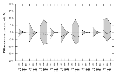
Figure 5. $QC$-criterion without tie breaking

As the figure shows, it might be possible to have a good tie-breaking routine which gives a better success rate than that of neighbor-joining. We believe that a deeper understanding of tie-breaking routine of the QCC algorithm should have more results in this direction.

Conclusion

The behavior of the QCC algorithm is similar to that of neighbor-joining. From this similarity QCC reflects the qualitative nature of neighbor-joining and that of dissimilarity maps from DNA sequence data. The QCC algorithm has the same $l_{\infty}$ radius $\frac{1}{2}$ as neighbor-joining, and it requires only the quartet consistency condition to reconstruct a correct tree.

References

- Atteson, (1999) Atteson, K. 1999. The performance of Neighbor-Joining methods of phylogenetic reconstruction. Algorithmica, 25(2–3):251–278.
- Bryant, (2005) Bryant, D. 2005. On the uniqueness of the selection criterion in Neighbor-joining. J. Classification, 22(1):3–15.
- Bryant and Steel, (2001) Bryant, D. and Steel, M. 2001. Constructing optimal trees from quartets. J. Algorithms, 38(1):237–259.
- Buneman, (1971) Buneman, P. 1971. The recovery of trees from measures of dissimilarity. In Hodson, F. R., Kendall, D. G., and Tautu, P., editors, Mathematics in Archeological and Historical Sciences, pages 387–395. Edinburgh University Press.
- John et al., (2003) John, K. S., Warnow, T., Moret, B., and Vawter, L. 2003. Performance study of phylogenetic methods: (unweighted) quartet methods and neighbor-joining. J. Algorithms, 48(1):173–193.
- Levy et al., (2006) Levy, D., Yoshida, R., and Pachter, L. 2006. Beyond pairwise distances: neighbor-joining with phylogenetic diversity estimates. Mol. Biol. Evol., 23(3):491–498.
- Mihaescu et al., (2006) Mihaescu, R., Levy, D., and Pachter, L. 2006. Why neighbor-joining works. arXiv.org:cs/0602041.
- Rambaut and Grassly, (1997) Rambaut, A. and Grassly, N. 1997. Seq-Gen: An application for the Monte Carlo simulation of DNA sequence evolution along phylogenetic trees. Comput. Appl. Biosci., 13:235–238.
- Saitou and Nei, (1987) Saitou, N. and Nei, M. 1987. The neighbor-joining method: A new method for reconstructing phylogenetic trees. Mol. Biol. Evol., 4(1):406–425.
- Studier and Keppler, (1988) Studier, J. A. and Keppler, K. J. 1988. A note on the neighbor-joining method of Saitou and Nei. Mol. Biol. Evol., 5:729–731.