Correlation entropy of synaptic input-output dynamics

Abstract

The responses of synapses in the neocortex show highly stochastic and nonlinear behavior. The microscopic dynamics underlying this behavior, and its computational consequences during natural patterns of synaptic input, are not explained by conventional macroscopic models of deterministic ensemble mean dynamics. Here, we introduce the correlation entropy of the synaptic input-output map as a measure of synaptic reliability which explicitly includes the microscopic dynamics. Applying this to experimental data, we find that cortical synapses show a low-dimensional chaos driven by the natural input pattern.

I Introduction

The excitatory cortical synapse is an example of a nonlinear biological system with a high level of intrinsic noise. This leads to a complex relationship between the input – the times of presynaptic action potentials (APs) – and the output – the variable amplitudes of excitatory postsynaptic potentials (EPSPs). The underlying mechanisms of this dynamics are not well understood. However, cortical synaptic transmission has been studied extensively by measuring the ensemble mean responses to short stimulus trains. Such responses show short-term ‘plasticity’ or activity–dependent changes, both augmenting and depressing Tsodyks and Markram (1997); Abbott et al. (1997); Varela et al. (1997); Dobrunz and Stevens (1997); Thomson (1997), as do measurements of field potentials, which represent the spatial average of EPSPs in a large population of synapses, all driven with the same timing Dobrunz and Stevens (1999).

Current models of the dynamics of short-term plasticity are mean-field approximations Tsodyks and Markram (1997); Abbott et al. (1997); Varela et al. (1997), systems of deterministic differential equations describing the average flux of transmitter between different functional pools. In this treatment, the large ‘synaptic noise’ around the ensemble mean of individual responses is considered to be extrinsic to the underlying dynamics of the synaptic response. In fact, though, it is known that the trajectory of individual responses contains a large amount of (at least short-term) predictability or determinism which is lost by the averaging of responses. For example, immediately following a failure to release transmitter in response to a presynaptic spike, there is a greatly raised probability of release at a closely-subsequent spike, and vice versa (e.g. Stevens and Wang (1995)).

As a consequence, characterizing the input-output dynamics of the synapse by the deterministic dynamics of the ensemble mean does not capture the full predictability of the synapse. From a neurobiological point of view, a useful goal in understanding the operation of neural circuits is to estimate the rate at which predictability is lost, or equivalently the rate of production of new information by the dynamics of individual synapses, during natural sequences of input. Our aim here is to do this in a way which captures nonlinear correlations in the fluctuations around ensemble mean responses, which embody much of the predictability of synaptic transmission. In addition, this will shed light on the dynamical nature of synaptic transmission. For example, do the noise of the input and the intrinsic noise of the synapse result in behavior like stochastic chaos Rand and Wilson (1991)? In this study, we describe a general, nonlinear approach to this problem, using the correlation entropy of the input-output map of the synapse.

II Correlation entropy estimated from input-output time series

A sequence of synaptic responses to an arbitrarily-timed spike-train input may be thought of as a map from input-output history to the amplitude of the next event:

$$\mathbf{h_{i}}\mapsto A_{i+1}$$ (1)

where

$${\bf h}_{i} =[{\bf A}_{i}^{m};{\bf{\Delta t}}_{i}^{n}]$$

$$=[A_{i-m+1},A_{i-m+2},.....,A_{i},$$ (2)

$$\hskip 12.91663pt\Delta t_{i-n+1},\Delta t_{i-n+2},.....\Delta t_{i}]$$

and $m$ is the number of amplitude dimensions, $n$ is the number of interspike interval dimensions in the history, $\mathbf{A}$ represents the amplitudes and $\mathbf{\Delta t}$ the intervals preceding each response. Equivalently, $\mathbf{h_{i}}\mapsto\mathbf{h_{i+1}}$ defines the dynamics in an input-output time delay space (see Cao et al. (1998a, b)).
The correlation entropy $K_{2}$ is a lower bound for the Kolmogorov-Sinai entropy of a dynamical system Grassberger and Procaccia (1983), which can be calculated from correlation sums. We extend the definition given in Grassberger and Procaccia (1983) to this bivariate, input-output process, distinguishing input (time intervals) and output (amplitude) dimensions. Let

$$\mu=\ln\frac{C(m,n,\delta,\epsilon)}{C(m+1,n+1,\delta,\epsilon)}-\ln\frac{C(n,\delta)}{C(n+1,\delta)}.$$ (3)

The first term is the correlation exponent for the joint input–output process, while the second term is that for the input process alone. Then the correlation entropy of the input–output process

$$K_{2}=\lim_{m,n\rightarrow\infty}\lim_{\delta,\epsilon\rightarrow 0}\lim_{N\rightarrow\infty}\mu(m,n,\delta,\epsilon)$$ (4)

where $N$ is the number of data points. The correlation sums are given by

$$C(m,n,\delta,\epsilon)=\frac{2}{N(N-1)}\times$$

$$\sum_{i=1}^{N}\!\sum_{j=i+1}^{N}\Theta(\epsilon\!-\|\mathbf{A}_{i}^{m}\!-\!\mathbf{A}_{j}^{m}\|)\Theta(\delta-\!\|\mathbf{\Delta t}_{i}^{n}-\mathbf{\Delta t}_{j}^{n}\|)$$ (5)

$$C(n,\delta)=\frac{2}{N(N-1)}\sum_{i=1}^{N}\!\sum_{j=i+1}^{N}\Theta(\delta-\!\|\mathbf{\Delta t}_{i}^{n}-\mathbf{\Delta t}_{j}^{n}\|)$$ (6)

where $\Theta$ is the Heaviside step function, $\|\cdots\|$ denotes the maximum norm and $\epsilon$ and $\delta$ are the neighborhood extents in amplitude and interval dimensions respectively. $K_{2}$ measures the uncertainty per synaptic event in the postsynaptic potential from the entire dynamics of synaptic transmission while subtracting the input uncertainty. It is useful to examine the convergence behavior of $\mu$, the estimate of $K_{2}$, as a function of the output neighborhood size $(\epsilon)$. As the neighborhood shrinks, $\mu$ for stochastic processes approaches infinity, or for chaotic deterministic processes, a finite positive value Gaspard and Wang (1993); Schittenkopf and Deco (1997); Faure and Korn (1998). For small extrinsic noise, for example, it is in principle possible to separate the entropy that is due to deterministic dynamics from the noise, and to estimate the noise level as the neighborhood radius below which $\mu$ starts to rise sharply.

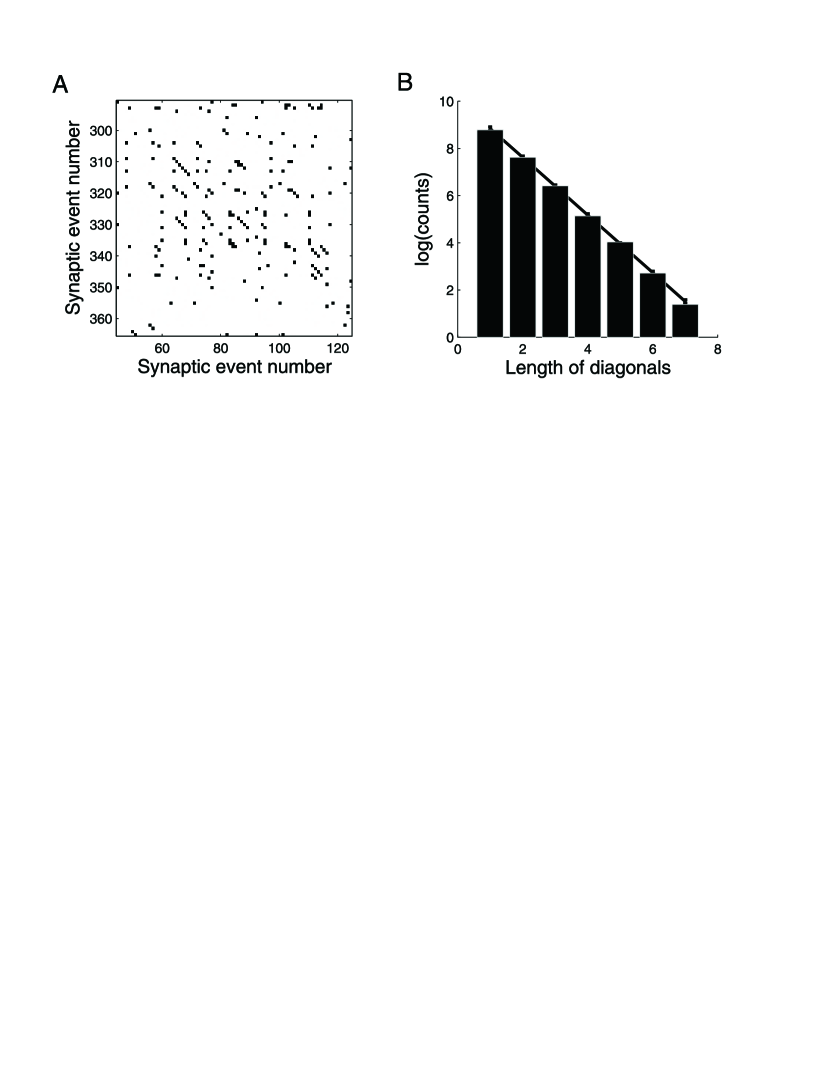
Figure 1: Input-output recurrence plot of synaptic transmission data. Stimulation parameters as in Fig. 3B, D–E. A: Excerpt of a recurrence plot for neighborhood dimensions $\epsilon=0.35$ mV, $\delta=290$ms. Matrix elements $[i,j]$ are colored black when $\Theta(\epsilon-\|\mathbf{A}_{i}-\mathbf{A}_{j}\|)\Theta(\delta-\|\mathbf{\Delta t}_{i}-\mathbf{\Delta t}_{j}\|)=1$. $m=n=2$. B: Cumulative logarithmic histogram of diagonal lengths in a recurrence plot of a complete time series (30 mins). The correlation exponent of the joint input–output process is estimated from the slope of this plot (1.75).

We used a method that estimates $\mu$ from the slopes of the logarithmic distributions of diagonal lengths in recurrence plots (RP)Faure and Korn (1998), rather than directly from Eqns. (5,6). The RP is a matrix representing similarity in local history between all pairs of embedding points in a time series (Fig. 1A). This method is robust against slow nonstationarity in the data Webber Jr. and Zbilut (1994), and is also computationally efficient, since it requires only one calculation of the distances between points at a low embedding dimension. As expected, the distributions of diagonal lengths could be fitted very well with an exponential, allowing unambiguous measurement of the correlation exponents (Fig. 1B).

III The noise-driven logistic map

In this section we illustrate the method using the logistic map perturbed with noise in each iteration. This is given by

$$x_{i+1}=\|a(x_{i}+\xi_{i})(1-x_{i}-\xi_{i})\|\;\mathrm{mod}\;1$$ (7)

Here the noise values $\xi_{n}$, drawn randomly from a Gaussian distribution with a standard deviation $\sigma_{\xi}$, correspond to the input time series $\Delta t_{i}$ above. Analogously the output time series is given by the set of $x_{n}$, corresponding to the set of $A_{i}$.

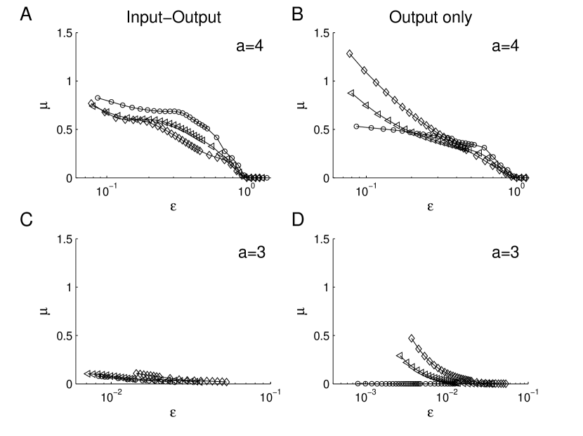
Figure 2: Input-output correlation entropy of the noise-driven logistic map (eqn. 7). Time series consisted of 5000 points, and results from 500 trials were averaged. Symbols denote various noise levels relative to the standard deviation of the unperturbed map $\sigma_{\xi}/\sigma_{up}$: $\diamond=0.5$, $\lhd=0.25$, $\circ=0.01$, $m=n=6$. $x_{0}=0.7$, $a=4$ (A,B) and $a=3$ (C,D). A: $\mu$ as a function of $\epsilon$ for $\delta\rightarrow 0$ B: $\mu$ as a function of $\epsilon$ estimated solely from the output time series ($\delta\rightarrow\infty$). C: As A but for $a=3$ D: As B but for $a=3$.

First, we chose $x_{0}=0.7$ and $a=4$, which produces a chaotic process in the unperturbed case.

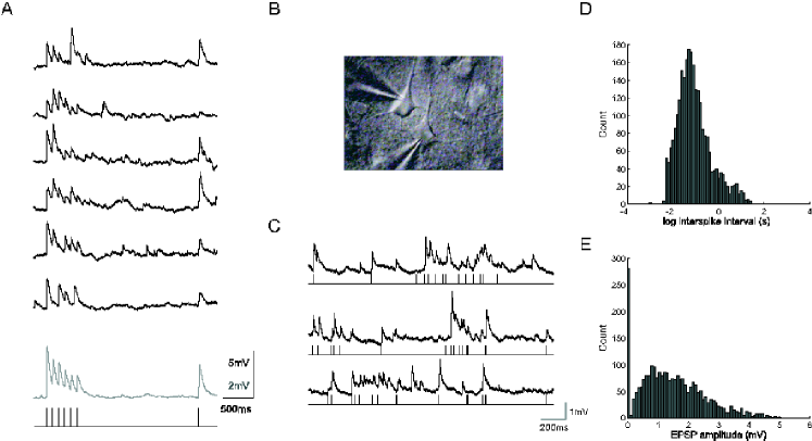
Figure 3: Synaptic transmission at a cortical synapse. A: 6 consecutive postsynaptic responses (top) and ensemble mean response (bottom, 50 responses) to the presynaptic stimulation pattern indicated below. B: Whole-cell recording in synaptically coupled pyramidal neurons of the rat cortex. C: A segment of a continuous recording showing evoked and spontaneous EPSPs (upper traces) during naturalistic stimulation (APs in lower traces) with parameters: $R_{p}=30$Hz $\lambda_{b}=0.2$Hz $\tau_{b}=200$ ms, average rate 1.2 Hz (see text). D, E: Corresponding distributions of interspike intervals (D) and postsynaptic EPSP amplitudes (E) for an experiment lasting 30 minutes.

The profile of the convergence of $\mu$ as $\epsilon$, the output neighbourhood radius, approaches zero is illustrated in Fig. 2, at three different strengths of the driving noise $\sigma_{\xi}$. Fig. 2A shows the profile for the input-output correlation entropy. When $\delta$ approaches zero (in this case, $\delta=9\cdot 10^{-5}$), i.e. when input dimensions are included in the trajectories for the entropy estimation, $\mu$ clearly converges to a plateau value. In contrast, for $\delta=\infty$, i.e. when the input dimensions are ignored and $\mu$ is calculated conventionally from the $x_{i}$ alone, convergence to a plateau is not apparent except at almost zero perturbation amplitude (Fig. 2B), since it is masked by the effect of the ‘unknown’ input noise, which causes $\mu$ to rise as $\epsilon\rightarrow 0$ (see Faure and Korn (1998) for discussion). Thus using the input-output method can use process noise when it is actually known, i.e. when it is ‘input’, to expose the low-dimensional dynamics of the driven process. In a regime which is periodic in the noise-free case ($a=3$. Fig. 2C), $\mu$ is greatly reduced. The residual value reflects the finite number of embedding points used and decreases with increasing N. Note however, the driving input noise samples parts of the state space which are off the attractor, and in general, $\mu$ is not expected to be the same as that of the noise-free case. For example, with driving noise, a nonlinear system can spend large amounts of time near chaotic repellors in the phase space Rand and Wilson (1991). In the synapse the ‘unperturbed’ or unstimulated dynamics is trivially a fixed point of amplitude zero.

IV Synaptic transmission data

We carried out whole cell patch-clamp recordings in 21 pairs of synaptically-connected layer 2/3 pyramidal neurons (Fig. 3B), using standard techniques met . The amplitude of synaptic events showed a typical pattern of variability in repeated responses to short bursts, and short-term depression in the ensemble average (Fig. 3A). Next, presynaptic APs were stimulated continuously for periods of 30 minutes, with presynaptic spike timing determined by an inhomogeneous Poisson process Cox and Miller (1977) the rate of which was modulated in exponentially-decaying bursts (peak amplitude $R_{p}$, time constant $\tau_{b}$), at times generated by a stationary Poisson process of rate $\lambda_{b}$ (Fig. 3C). Such a process is thought to model the statistics of natural bursting synaptic input reasonably well, and can have a coefficient of variation of interspike intervals [CV(ISI)] greater than 1 Harsch and Robinson (2000). Postsynaptic responses to this stimulus train showed a high variability in amplitude, including a large proportion of failures, as well as asynchronous spontaneous events (Fig. 3C). Distributions of $\mathbf{\Delta t}$ and $\mathbf{A}$ are shown in Fig. 3D and Fig. 3E. Over 30 minutes of continuous stimulation at an average rate of 1.2 Hz, there is typically a small depressing trend in the average response amplitude, referred to as long-term depression Malenka and Siegelbaum (2001).

IV.1 Dispersion of future synaptic transmissions

A

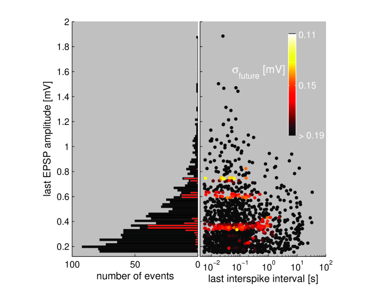
B

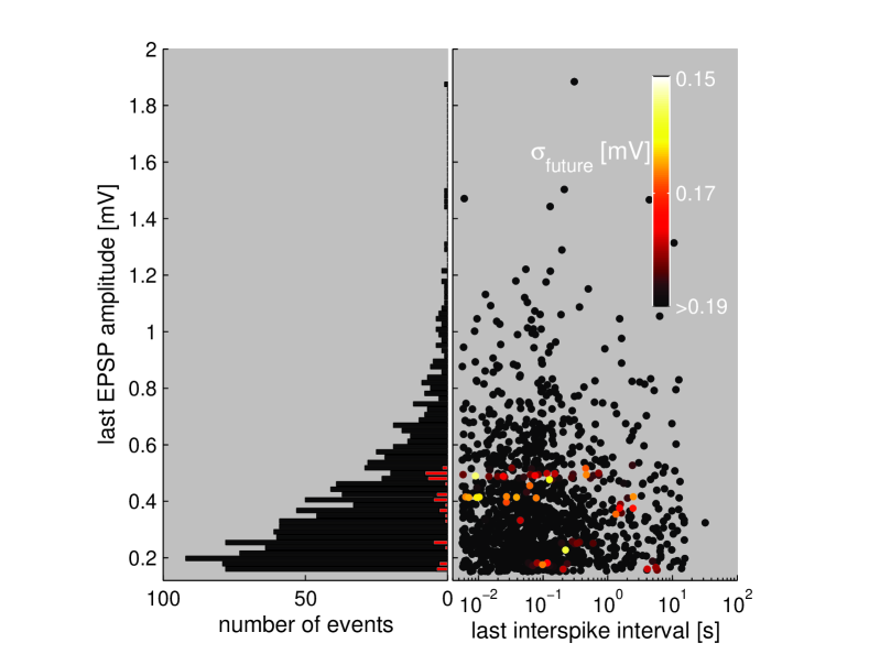
Figure 4: Clustering of amplitudes of responses with reliable futures. A: The history vector was defined only by the last interspike interval and last EPSP amplitude. Points are colour coded according to the dispersion value (see text) as indicated on the right using 50 nearest neighbours. Stimulus parameters were $R_{peak}=30\,\rm Hz$, $\tau_{b}=200\,\rm ms$ $\lambda_{b}=0.2\,\rm Hz$, which amount to an average rate of $1.2\,\rm Hz$. B: Control for A using a random permutation of the amplitude time series.

First, we show evidence of nonlinear structure in the highly variable input–output relationship of these synapses. To do this we searched for histories $\mathbf{h_{i}}$ with the most reliable futures $A_{i+1}$ (see Eqn.II). As a measure of the similarity between two histories, we used the Euclidian distance between their history-vectors after normalizing amplitude and interspike interval dimensions. For each event of the time series we computed $\mathcal{N}_{k}({\bf h_{i}})$, the set of the $k$ nearest neighbors of ${\bf h_{i}}$ope . The dispersion of the future output for a trajectory $\bf h_{i}$ can be characterized by $\sigma_{i}$, the standard deviation of the futures $\mathcal{N}_{k}({\bf h_{i}})$ and $\sigma_{A}$ the standard deviation of $\bf A$. A simple example of this analysis, which can be easily visualized, is to distinguish which combinations of most recent interspike interval and EPSP amplitude lead to small dispersions. The results are presented in Fig. 4A. In the right hand panel the distribution of all points in this space is shown (the range of the axes excludes failures). Points are colored according to their dispersions. Points with relatively reliable futures (low dispersion) are yellow or red. It is striking that the amplitude dimension of such points has a much tighter distribution than that of all amplitudes (see histogram in the left panel), and that values are clearly restricted to a few sharp peaks. This pattern was seen in 7 out of 8 synapses analyzed in this way. Shuffled surrogates (see Fig. 4B) never showed a similar pattern. Thus, within the complex and variable response of the synapse, a subset of patterns are transmitted with considerable precision. In this case for intervals less than the vesicle replenishment time constant of the synapse Markram and Tsodyks (1996); Varela et al. (1997), the amplitude of the preceding event has a greater impact than the interval. The $K_{2}$ entropy that we have defined above gives a global characterization of dispersion over all histories of input–output.

IV.2 Correlation entropy of synaptic data

Fig. 5A shows a typical portrait of the dependence of $\mu$ on the neighborhood size, $\epsilon$. As $\epsilon\rightarrow 0$, $\mu$ converges to a constant plateau value (solid black line). In surrogates where the output values are randomly shuffled, to destroy all correlations in the output, or shifted in time to destroy only the correspondence between the input and output, while preserving the correlations within the input and output individually, $\mu$ continues to grow as $\epsilon\rightarrow 0$. Theoretically this should approach $\infty$, but is prevented from doing so by the large number of zeros (failures) in the amplitude distribution (Fig. 3E). The small difference between the two surrogates described above indicates that there is little additional correlation in the output which is independent from the input, i.e. the synapse is highly driven, in this case.

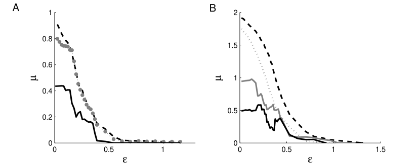
Figure 5: Convergence of $K_{2}$-entropy estimate $\mu$ for synaptic data. A: A typical $\mu(\epsilon)$ relationship at a very small $\delta=0.018$ms. A clear convergence is seen as $\epsilon\rightarrow 0$. Stimulation parameters as in Fig. 1. Total number of stimulation events in the time series was 2594. The mean of 50 randomly shuffled controls is shown as a dashed line. The standard deviation $\sigma$ of these controls was maximal for $\epsilon\rightarrow 0$, $\sigma<0.18$. Gray $\circ$ denotes the mean of 50 surrogates with a large shift between the amplitude and interspike interval time series (see text). A shift $>10$ minutes was randomly chosen, $\sigma<0.43$ B: $\mu(\epsilon)$ before and after induction of spike-timing dependent plasticity (STDP). Gray line denotes the data before the induction of STDP, black solid line denotes after induction. The means of 50 randomly shuffled controls are shown as corresponding dashed lines, $\sigma<0.44$ before STDP and $\sigma<0.43$ after STDP. Stimulation parameters were $\bar{R}=30$Hz $\lambda_{b}=0.5$Hz $\tau_{b}=400$ms, average rate 6 Hz. The stimulation before and after STDP induction was identical, with 3000 stimulation events.

Thus, a converging value for $\mu$ for small $\epsilon$ is clearly identifiable in cortical synapses, even for stochastic input patterns, and is a measure of the uncertainty produced by synaptic transmission.

$\mu$, being a measure of the information rate of the input-output dynamics of the synapse, ought to change when the properties of the synapse are altered via long-term plasticity, which is believed to underlie learning and memory. To test this, we applied a presynaptic–postsynaptic paired stimulus protocol Markram et al. (1997); Bi and Poo (2001), in which pre and postsynaptic APs are repeatedly stimulated with a 10 ms delay between them to allow coincident arrival of both at the synaptic terminal. After this so-called ‘spike-timing-dependent’ long-term potentiation, $\mu$ showed a similar form to the control distribution, but a clear shift to lower values in the low $\epsilon$ limit (Fig. 5B). In this sense, less uncertainty is being created by the synaptic transmission for the same statistics of input, i.e. reliability of transmission is enhanced for this stimulus process. Similar findings were seen in 5 synaptic connections.

IV.3 A biophysical model of short-term plasticity

To gain insight into possible underlying mechanisms, we also carried out the same analysis on a stochastic biophysically-based microscopic model of cortical synapses adapted from Fuhrmann et al. (2002). In this model, which is consistent with a mean-field deterministic model of short-term plasticity Tsodyks and Markram (1997), the stochastic release and replenishment of a small pool of transmitter vesicles (‘quanta’) is simulated explicitly, with Gaussian variability of vesicle amplitude. The synaptic connection is composed of $N$ release sites. At each site there may be, at most, one vesicle available for release, and the release from each of the sites is independent of the release from all other sites. The dynamics is characterized by two probabilistic processes, release and recovery. At the arrival of a presynaptic spike at time $ts$, each site containing a vesicle will release the vesicle with the same probability, $U_{se}$ (use of synaptic efficacy). Once a release occurs, the site can be refilled (recovered) during a time interval $\Delta t$ with a probability $1-e^{-\Delta t/\tau_{rec}}$, with $\tau_{rec}$ as a recovery time constant. Both processes can be described by a single differential equation, which determines the ensemble probability, $P_{v}$, for a vesicle to be available for release at any time $t$ Fuhrmann et al. (2002).

$$\frac{dP_{v}}{dt}=\frac{1-P_{v}}{\tau_{rec}}-U_{se}\cdot P_{v}\cdot\delta(t-ts)$$ (8)

The iterative solution for a train of spikes arriving at one release site is given by

$$P_{v}(ts_{i+1})= P_{v}(ts_{i})\cdot(1-U_{se})$$

$$\times\, e^{-(ts_{i+1}-ts_{i})/\tau_{rec}}+1-e^{-(ts_{i+1}-ts_{i})/\tau_{rec}}$$ (9)

where $ts_{i}$ is the $i^{th}$ spike time, and $P_{r}(ts_{i})=U_{se}\cdot P_{v}(ts_{i})$ denotes the probability of release for each release site at the time of a spike $ts_{i}$.
However, individual trajectories follow a different dynamics from the ensemble since at each spike time $ts$ an all-or-nothing stochastic decision is made on the availability of a vesicle, and therefore the release probability set back to zero if release occurs. Thus individual realizations follow an abruptly changing, nonlinear stochastic map. Individual trajectories were simulated as follows: for each individual release site, the times of the most recent transmitter release ($tr_{i}$) are recursively defined for a given input time series of spike times ($ts_{i}$)

$$tr_{i+1}= tr_{i}+(ts_{i+1}-tr_{i})$$

$$\times\, \Theta(ts_{i+1}-tr_{i}-\tau_{i})\Theta(U_{se}-\xi_{i+1})$$ (10)

with the associated refilling intervals:

$$\tau_{i+1}=\Pi_{i}\tilde{\Theta}(tr_{i+1}-tr_{i})+\tau_{i}\Theta(tr_{i}-tr_{i+1})$$ (11)

where $\Pi_{i}$ is a random number from an exponential distribution with a time constant $\tau_{rec}$ (see 8), $\xi_{i}$ a random number from a uniform distribution in the interval $[0;1]$, and

$$\Theta(x)=\left\{\begin{array}[]{cc}0&x<0\\ 1&x\geq 0\end{array},\right.$$

$$\tilde{\Theta}(x)=\left\{\begin{array}[]{cc}0&x\leq 0\\ 1&x>0\end{array}\right.$$

The postsynaptic response $a_{i}$ to a single vesicle release is assumed not to be a constant value but randomly drawn from a Gaussian distribution characterized by the coefficient of variation of the quantal content $CV(q)=\sigma_{q}/m_{q}$.

$$a_{i}=\zeta_{i}\sigma_{q}+m_{q}$$ (12)

where $\zeta_{i}$ is a random number from Gaussian distribution with mean 0 and a standard deviation of 1, and $\sigma_{q}$ is the standard deviation and $m_{q}$ the mean of the quantal content. Negative values for $a_{i}$ were rounded to zero. The final size of a postsynaptic response $A_{i}$ is the sum over all $N$ release sites

$$A_{i+1}=\sum_{j=1}^{N}a_{i}^{j}\tilde{\Theta}(tr_{i+1}^{j}-tr_{i}^{j})$$ (13)

In summary the model depends upon three stochastic processes, the recovery time for vesicles $\tau_{i}$, the decision whether to release $\Theta(U_{se}-\xi_{i})$, and the amount of transmitter released $a_{i}$.

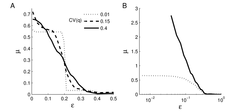
Figure 6: A: Analysis of a biophysically-based model of synaptic transmission Fuhrmann et al. (2002), driven by the same stimulus timing as used in Fig. 5A. The model parameters were: $U_{se}=0.5$, $\tau_{rec}=800$ ms, $N=5$, the mean quantal size $q=0.2$ mV for all release sites, see Fuhrmann et al. (2002) for details. Graphs are shown for three different levels of variability of the quantal content. B: Same analysis as in A but with a logarithmic scale in $\epsilon$ to demonstrate the divergence between the macroscopic mean-field model with additional extrinsic Gaussian noise (solid line) and the microscopic stochastic model (dotted line). The standard deviation of the Gaussian noise was estimated from average ensemble fluctuations of 1000 surrogates of the stochastic model (parameters as in A). The model parameters for the deterministic model were chosen accordingly: $U_{se}=0.5$, $A_{se}=1$, $\tau_{rec}=800$ms.

This model was able to reproduce a convergence of $\mu(\epsilon)$ for physiologically realistic parameters (Fig. 6A), although not as flat as the experimental data. When quantal variability was reduced to very low values, step-like patterns were observed in the $\mu(\epsilon)$ relationship, reflecting a reliable quantal representation (i.e. number of quanta) of EPSP amplitude. This indicates that the convergence of $\mu$ for real data might reflect deterministic predictability of quantal number. When we analyzed the corresponding macroscopic or mean-field model Tsodyks and Markram (1997) with additive Gaussian noise of the same amplitude as the average ensemble fluctuations, a very different pattern of $\mu(\epsilon)$ was observed (Fig. 6B). Instead of convergence at low $\epsilon$, $\mu$ rose sharply to arbitrarily high values as $\epsilon\rightarrow 0$. Thus the signature of this uncorrelated extrinsic noise added to the mean-field dynamics is quite different again from what is observed in the experimental data. The convergence of $\mu$ both in actual data and in the microscopic biophysical model, but not for the mean-field case with extrinsic noise, implies that the intrinsic microscopic nature of synaptic transmission leads effectively to a state of low-dimensional chaos.

Any classification of the nature of the dynamics in this way as chaotic or stochastic, using real time series of finite length, actually depends on the scale of $\epsilon$ and $\delta$ and the length of data available Cencini et al. (2000). In the nervous system, the postsynaptic cell has a limited resolution for distinguishing the amplitude (set by intrinsic channel gating noise) and timing (set by jitter in synaptic latencies) of individual synaptic events. These resolution limits, or the effective granularity of representation of amplitude and timing, will vary according to the location of the synapse on the dendritic tree and the state of activation of ion channels, which together determine the spatial and temporal filtering of inputs. Thus, the scale or $\epsilon$,$\delta$-dependence, of the correlation entropy measure should be meaningful physiologically in understanding the generation and flow of information in a neural circuit.

Previous work has characterized synaptic reliability using very low frequency single pulse trials (e.g. Feldmeyer et al. (2002)) or as the ensemble responses to short bursts of APs (e.g. Abbott et al. (1997); Tsodyks and Markram (1997); Dobrunz and Stevens (1997); Dittman et al. (2000); Gupta et al. (2000)). In contrast, the correlation entropy $K_{2}$ gives a measure of the overall nonlinear predictability of the microscopic input-output mapping of a synapse - driven by a particular, but arbitrary stimulus pattern, which can be calculated practically from synaptic data. It also has a simple information-theoretical interpretation as the rate of information or uncertainty production by a synapse. Therefore, it is a natural measure for characterizing the dynamic reliability of a synapse during natural activity. Applying it to experimental results suggests that the microscopic characteristics of transmitter release and postsynaptic receptor kinetics, combined with a complex natural-like input timing, lead to a stochastic chaotic process at individual cortical synapses, at certain scales of resolution.