Elementary simulation of tethered Brownian motion

Abstract

We describe a simple numerical simulation, suitable for an undergraduate project (or graduate problem set), of the Brownian motion of a particle in a Hooke-law potential well. Understanding this physical situation is a practical necessity in many experimental contexts, for instance in single molecule biophysics; and its simulation helps the student to appreciate the dynamical character of thermal equilibrium. We show that the simulation succeeds in capturing behavior seen in experimental data on tethered particle motion.

I Introduction and summary

Introductory courses in statistical physics often place their greatest emphasis on average quantities measured in thermodynamic equilibrium. Indeed, the study of equilibrium gives us many powerful results without having to delve into too much technical detail. This simplicity stems in part from the fact that for such problems, we are not interested in time dependence (dynamics); accordingly dissipation constants like friction and viscosity do not enter the formulas.

There are compelling reasons, however, to introduce students to genuinely dynamical aspects of thermal systems as early as possible—perhaps even before embarking on a detailed study of equilibrium philbook . One reason is that students can easily miss the crucial steps needed to go from a basic appreciation that “heat is motion” to understanding the Boltzmann distribution, and thus can end up with a blind spot in their understanding of the foundations of the subject. Although any kind of rigorous proof of this connection is out of place in a first course, nevertheless a demonstration of how it works in a sample calculation can cement the connection.

A second reason to give extra attention to dynamical phenomena is the current surge in student interest in biological physics. Much current experimental work studies the molecular processes of life, or their analogs, at the single-molecule level, where simple mathematical descriptions do seem to capture the observed behavior.

One familiar setting where simple models describe statistical dynamics well is the theory of the random walk, and its relation to diffusion. Ref. philbook showed an attempt to present classical statistical mechanics starting from the random walk, building on earlier classics such as Ref. Bberg93a . The link between thermal motion and the Boltzmann distribution emerges naturally in the analysis of sedimentation equilibrium: We require that in equilibrium, diffusive changes in a concentration distribution must cancel changes caused by drift from a constant external force field (gravity).

In this article we discuss a generalization of free Brownian motion that is important for interpreting a large class of current experiments in single-molecule biophysics: The Brownian motion of a particle tethered to a Hookean spring. Specifically, we investigate the dynamics of fluctuations of such a particle in equilibrium. Although the theoretical analysis of this problem does appear in some undergraduate textbooks, it sometimes appears forbiddingly complex (e.g. Ref. Breif65a ). We have found, however, that numerical simulation of the system is well within the range of an undergraduate project. Either as a project or a classroom demonstration, such a simulation brings insight into the emergence of equilibrium behavior from independent random steps, and also can serve as an entry into the topic of equilibrium fluctuations.

The appendix gives an implementation written by one of us, an undergraduate at Ursinus College, in matlab.

II Experimental background

As motivation, we briefly mention two contexts in which Brownian motion in a harmonic (Hooke-law) trap has played a role in recent biological physics experiments.

Optical trappinggitt97a ; philbook is now an everyday tool for the manipulation of micrometer-scale objects (typically a polystyrene bead), and indirectly of nanometer-scale objects attached to them (typically DNA, RNA, or a protein). In this method, a tightly focused laser spot creates a restoring force tending to push a bead toward a particular point in space. When the trapping beam has a Gaussian profile, the resulting force on the bead is often to a good approximation linear in bead displacement. Thus the bead executes Brownian motion in a harmonic potential well. In such a well the motions along the three principal axes of the well are independent.

The bead’s motion in one or two dimensions can be tracked to high precision, for example by using interferomotry, thus yielding a time series. The probability distribution of the observed bead locations then reflects a compromise between the restoring force, pushing the bead to the origin, and thermal motion, tending to randomize its location. The outcome of this compromise is a Gaussian distribution of positions, from which we can read the strength of the harmonic restoring force (“trap stiffness”). For practical reasons, however, it is often more accurate to obtain both trap stiffness and the bead’s effective friction constant from the autocorrelation function of the bead position (see Sect. IV below). For example, slow microscope drift can spoil the observed probability distribution function (see Ref. gitt97a ).

Our second example concerns tethered particle motionfinzi95 . In this technique, a bead is physically attached to a “tether” consisting of a long single strand of DNA. The other end of the tether is anchored to a microscope slide and the resulting bead motion is observed. Changes in the bead’s motion then reflect conformational changes in the tether, for example the binding of proteins to the DNA or the formation of a long-lived looped state. Fig. 1a shows example data for a situation where such conformational changes are absent, that is, simple tethered particle motion.

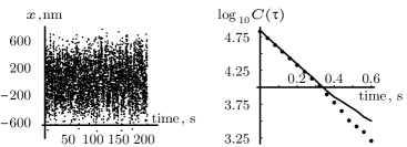
Figure 1: Left, sample experimental data for the $x$-component of the motion of a bead of radius $R_{\rm bead}\approx 240\,$nm, attached to a DNA tether of length $L_{\rm tether}\approx 3500$ basepairs, or $\approx 1200\,$nm. The experiment, and the protocols used to remove drift from the raw data, are described in detail in Ref. nels06a . For clarity only the first 200 s of data are shown; the full data run lasted 600 s. Right, logarithm of the autocorrelation function of $x$ expressed in nm² (see text). Solid line, experimental data. Dots, simulation described in this paper, using parameters $A_{\rm eff}=72\,$nm and effective viscosity 2.4 times that of water in bulk. [f:tpm]

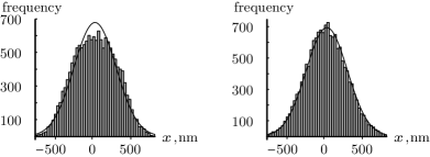
Figure 2: Left, histogram of measured bead $x$ position for the experimental data shown in Fig. 1. The solid curve shows a Gaussian distribution with the same normalization and variance. Right, similar histogram for our simulation. [f:histo]

As in the optical trap case, one can discard the dynamical information in the time series by making a histogram of particle locations. Fig. 2a shows the frequencies of occurence of various values of $x$. Rather detailed agreement between theory and experiment has been obtained for these histograms, including the slight deviation from Gaussian distribution shown in the figuresega06a ; nels06a . In the present note, however, we are interested in a less sophisticated treatment of a more general question: Can we understand at least some aspects of the dynamical information contained in data like those in Fig. 1?

To this end, Fig. 1b shows the logarithm of the autocorrelation function, $C(\tau)\equiv\langle x(t+\tau)x(t)\rangle$, where the brackets denote averaging over $t$. At $\tau=0$ this quantity is just the meansquare displacement, which would diverge for a free particle but instead has a finite value determined by the equipartition theorem. At large times the autocorrelation falls to zero, because two independent measurements of $x$ are as likely to lie on opposite sides of the tethering point as they are to lie on the same side. In fact, the autocorrelation function should fall exponentially with $\tau$, as we see it does in Fig. 1b.Breif65a

III Simulation setup

We wish to simulate the motion of a bead of radius $R_{\rm bead}$, attached to a tether of length $L_{\mathrm{tot}}$, and compare our results to experimental data. For this we will need to know a specific property of DNA in typical solution: Its “persistence length” $A$ is $A\approx 45\,$nm.philbook

We will suppose that the external forces acting on the bead are a hard-wall repulsion from the microscope slide, a tension force from the tether, and random collisions with surrounding water molecules (see Sect. V for further discussion). The tension force produces an effective potential well that keeps the bead close to its attachment point. In fact, at low relative extension, the tension exerted by a semiflexible polymer like DNA is approximately given by a Hooke-type law:philbook $f=-\kappa x$. The effective spring constant is $\kappa=3{k_{\rm B}T}/(2AL_{\mathrm{tot}})$, where ${k_{\rm B}T}\approx 4.1\cdot 10^{-21}\,$J is the thermal energy at room temperature and $L_{\mathrm{tot}}$ is the contour length of the polymer. Thus, again the motions in each of the $x$, $y$, and $z$ directions are independent. Because the microscopy observes only $x$ and $y$, we can reduce the problem to a two-dimensional one, and hence forget about the hard-wall force, which acts only along $z$. In fact, we will reduce it still further, by examining only the $x$ coordinate of the bead position.

There is a subtlety in that we do not directly observe the endpoint of the polymer in an experiment. Rather, we observe the image of the bead; the image analysis software reports the location of the bead center, a distance $R_{\rm bead}$ from the attachment point. Thus the time series in Fig. 1a reflects the motion of the endpoint of a composite object, a semiflexible polymer attached by a flexible link to a final, stiff segment of length $R_{\rm bead}$. To deal simply with this complication, we note that a semiflexible polymer can also be approximately regarded, for the purposes of finding its force–extension relation, as a chain of stiff segments of length $2A$. In our case $2A\approx 100\,$nm is not much larger than $R_{\rm bead}$, so we will approximate the system as a single Hookean spring, with effective length $L_{\mathrm{tot}}=L_{\rm tether}+R_{\rm bead}$ and an effective persistence length $A_{\rm eff}$ slightly larger than $A$. In the data we present, $L_{\rm tether}\approx 3500$ basepairs, or $\approx 1200\,$nm. We will fit the data to obtain $A_{\rm eff}$.

Suppose we observe the bead at time intervals of $\Delta t$. Without the tether, the bead would take independent random steps, each a displacement drawn from a Gaussian distribution with mean-square step length $2D(\Delta t)$, where $D$ is the bead’s diffusion constant. If the bead were subjected to a constant force $f$ (for example gravity), we could get its net motion by superimposing an additional deterministic drift on the random steps: $\Delta_{\rm drift}x=f/\zeta$. The friction constant $\zeta$ is related to $D$ by the Einstein and Stokes relations: $\zeta={k_{\rm B}T}/D=6\pi\eta R_{\rm bead}$, where $\eta$ is the viscosity of water. For the tethered case, at each step we instead use a position-dependent force $-\kappa x$, where $x$ is the current displacement. For small enough $\Delta t$ (perhaps smaller than the actual video frame rate), $x$ will be roughly constant during the step, justifying this substitution.

Here again we find a subtlety: The presence of the nearby wall creates additional hydrodynamic drag on the bead happ83a ; scha06a . Moreover, the tether itself incurs significant hydrodynamic drag impeding the system’s motion. Again for simplicity, we acknowledge these complications by fitting to obtain an effective viscosity $\eta_{\rm eff}$, which we expect to be larger than the value $10^{-3}\,$Pa s appropriate to water in bulk.

IV Simulation results[s:sr]

To summarize, the simulation implements a Markov process. Each step is the sum of a random, diffusive component with meansquare $2D(\Delta t)$, and a drift component $-D\kappa x/{k_{\rm B}T}$. The constants $D={k_{\rm B}T}/(6\pi\eta_{\rm eff}R_{\rm bead})$ and $\kappa=3{k_{\rm B}T}/(2A_{\rm eff}L_{\mathrm{tot}})$ contain two unknown fit parameters, the effective persistence length $A_{\rm eff}$ and viscosity $\eta_{\rm eff}$. The output of the simulation is the probability distribution of positions, and the autocorrelation function, which may be compared to experimental data.

The simulation is deemed successful to the extent that the two fit parameters take values reasonably close to the expected values, differing in the expected directions, and the full functional forms of the outputs agree with experimental data. Figures Fig. 1b and Fig. 2 show that indeed the simple model works well. Our simulation took $\Delta t=0.625\,$ms, for a total of about a million steps, which were then sampled every 40 ms to resemble the experimental data.

V Discussion[s:d]

Our mathematical model made some naive simplifications. Two which have been mentioned involve the role of the bead radius, and certain sources of drag on the bead. In addition, there is a time scale for rearrangements of the DNA needed to change its extension, and for rotatory diffusion of the bead, which changes the location of the attachment point relative to its center. All of these effects have been assumed to be lumped into effective values of the fit parameters.

Despite these simplifications, however, we did obtain two key qualitative aspects of the experimental data as outputs from the model, not set by hand. First, the autocorrelation function of equilibrium fluctuations has the expected exponential form. Moreover, as a consistency check, the experimental histogram of bead positions had roughly the Gaussian form we would expect for motion in a Hookean potential well. Both of these results emerge as statistical properties of a large number of simple steps, each involving only a diffusive step combined with a drift step based on the current bead location.

The insights obtained from this exercise are different from those obtained from the analytical solution; for example, students can see the average behavior emerging from the random noise as the simulation size grows. In addition, the simulation approach opens the door to replacing the assumption of a harmonic potential by any other functional form.

Appendix A Matlab code

function TetheredParticleAnalysis (Xdata,Ncorr,Nbins,deltat)
%This function simulates and analyzes the motion of a 1D random walk
%confined in a harmonic potential well.
%
%Written by Luke Sullivan, Ursinus College
%Edited by John F. Beausang, University of Pennsylvania
%
%Xdata    = array of bead position (nm)
%nCorr    = number of points in correlation function
%Nbins    = number of histogram bins
%deltat   = time step of data and simulation (sec)

%%%%Experimental Data%%%%
Xdata     = transpose(Xdata);
n         = length(Xdata);    %number of data points
time      = (1:n)*deltat;     %time series
[FData,rData,histoData] = GaussHistoX(Xdata,Nbins);
logACData = LogAutoCorr(Xdata,Ncorr,deltat);

%%%%Simulated data%%%%
Xsim = RandWalkSim(length(Xdata),deltat);  %generate simulated data
[FSim,rSim,histoSim] = GaussHistoX(Xsim,Nbins);
logACSim = LogAutoCorr (Xsim,Ncorr,deltat);

%%%%output%%%%
subplot(2,3,1);plot(time,Xdata,’b’)%Experimental data
title (’Experimental data’);
xlabel (’Time (sec)’);
ylabel (’Bead Position (nm)’);
subplot(2,3,2);plot(rData,FData,’bx’,histoData(1,:),histoData(2,:),’bo’)%Gaussian curve
title (’Gaussian fit (x) and Histogram (o) of exp data’);
xlabel (’position (nm)’);
ylabel (’Probability (1/nm)’);
subplot(2,3,4);plot(time,Xsim,’r’)%Simulated data
title (’Simulated data’);
xlabel (’Time (sec)’);
ylabel (’Bead Position (nm)’);
subplot(2,3,5);plot(rSim,FSim,’rx’,histoSim(1,:),histoSim(2,:),’ro’)%Gaussian curve
title (’Gaussian fit (x) and Histogram (o)of Sim data’);
xlabel (’position (nm)’);
ylabel (’Probability (1/nm)’);
subplot(2,3,3);plot(logACData(1,:),logACData(2,:),’b-’,logACSim(1,:),logACSim(2,:),’r-’)%plot of correlation function of data
title (’Compare AutoCorrelation’);
xlabel (’time difference (sec)’)
ylabel (’Log[AutoCorrelation], (nm2)’)

%%%%Subroutines%%%%%

function [F,r,Xhisto]=GaussHistoX (Xdata,Nbins)
%This function histograms the data and fits a Gaussian distribution
Xmax        = max(abs(Xdata));  %maximum position
n           = length(Xdata);    %number of data points
binWidth    = Xmax/Nbins;       %histogram bin width
stdevX      = std(Xdata);       %standard deviation of data
F=zeros(1,n);r=zeros(1,n);Xhisto=zeros(2,Nbins+1);  %initialize
Xhisto(1,:)= ((1:Nbins+1)-.5)*binWidth;     %midpoint of histogram bins
for i=1:n
    r(i)=abs(Xdata(i));
    F(i)=2/sqrt(2*pi*stdevX^2)*exp(-(Xdata(i)^2)/(2*stdevX^2));%1 sided gaussian curve
    which=1+floor(abs(Xdata(i))/binWidth);  %which bin data falls into
    Xhisto(2,which)=Xhisto(2,which)+1;      %increment bin
end
Xhisto(2,:)=Xhisto(2,:)/n/binWidth; %convert counts to probability (1/nm)

function logac = LogAutoCorr (Xdata,Ncorr,deltat)
%This function determines the autocorrelation of the data for Ncorr points
n         = length(Xdata);
logac     = zeros(2,Ncorr);
logac(1,:)= (0:Ncorr-1)*deltat;      %time steps
for s = 1:Ncorr
    temp = zeros (1,n-s+1);
    for i=1:(n-s+1)
        temp(i)=Xdata(i)*Xdata(i+s-1);
    end
    logac(2,s)=log10(sum(temp)/(n-s+1));
end

function Xsim=RandWalkSim(n,deltat)
%This function simulates a 1D random walk in a harmonic potential
%%%%physical parameters%%%%
L       = 3477*.34;         %tether length (nm)
Xi      = 72;               %tether persistence length (nm)
Rb      = 240;              %bead radius (nm)
kbT     = 4.1*10^(-21);     %thermal energy (J)
eta     = 2.4*10^(-30);     %viscosity of H2O (J*s/nm^3)
D       = kbT/(6*pi*eta*Rb);%Stokes diffusion constant (nm2/s)
kappa   = 3/2*kbT/Xi/L;     %spring constant (J/nm2)
mu      = D*kappa/kbT*deltat;%bias of step in harmonic potential
ldiff   = sqrt(2*D*deltat); %diffusion length (nm)

Xsim=zeros(1,n);
for i=2:n
    deltaX=randn(1)*ldiff-Xsim(i-1)*mu;%step size for each element called
    Xsim(i)=Xsim(i-1)+deltaX;%new element value
end