Dynamical Structure Functions for the Estimation of LTI Networks with Limited Information

Abstract

This research explores the role and representation of network structure for LTI Systems. We demonstrate that transfer functions contain no structural information without more assumptions being made about the system, assumptions that we believe are unreasonable when dealing with truly complex systems. We then introduce Dynamical Structure Functions as an alternative, graphical-model based representation of LTI systems that contain both dynamical and structural information of the system. We use Dynamical Structure to prove necessary and sufficient conditions for estimating structure from data, and demonstrate, for example, the danger of attempting to use steady-state information to estimate network structure.

I Introduction

One of the fundamental issues for modeling, identifying, and controlling complex networked systems is inferring system structure from input-output data. Structure is often the key for understanding a variety of complex systems because it enables a decomposition of the complete system into an interconnection of subsystems. When analysis of the subsystems is comparatively simple, and the interconnection structure is well understood, then the behavior of the complex system can be deduced from an understanding of its components. Moreover, exploiting structural information can tremendously reduce the conservatism of robust solutions designed to compensate for system uncertainty. This impact on complexity and uncertainty makes structural information extremely important in the analysis of complex networked systems.

Examples of scientists working on identifying or exploiting network structure arise in a variety of disciplines. Social scientists have developed a rich literature on the use of network models to describe interpersonal associations, perhaps one of the most famous works being Milgram’s ”small world” experiment in the 1960’s in which letters passed from person to person were able to reach a particular target individual in only about six steps [Milgram]. More recently, attention has focused on networks of business communities [Galaskiewicz, Mariolis, Mizruchi], internet-enabled virtual communities [Holme], citation networks in scientific communities [Redner, Seglen], preference networks for product recommender systems [Goldberg, Resnick], distribution networks [Amaral], and the detection and destabilization of terrorist networks [carley]. Epidemiologists have developed models for the dynamics of both epidemic and endemic diseases spreading through population networks [Hethcote], computer scientists have developed algorithms for searching over networks that are deployed in a number of popular applications [Brin], and biologists use microarray and other data sources to infer the regulation structure in genomic, proteomic, and metabolic networks [Guelzim, Maslov, Stelling, Uetz] .

Discovering structure from data, however, can be difficult. Typical identification methods do not emphasize structure estimation, but rather focus on behavior generalization by selecting a model that accurately predicts system outputs for unobserved inputs. As long as the dynamic behavior of the system is accurately described, the question of structure is often avoided altogether. For many applications, various model structures for the same input-output map are equally useful for forecasting and control. Nevertheless, sometimes it is important not only to describe the system dynamics accurately, but to do so with a model that correctly represents the structure of the original system.

In contrast with these identification methods that emphasize system dynamics over structure, inference methods have been developed that emphasize structure over dynamics. These methods employ graphical models to describe network structure. Nodes represent system states, understood to be random variables, and edges indicate conditional dependence between variables. Using Bayes rule, measurements can then be used to update prior distributions believed to characterize relationships throughout the network. A rich literature has grown in this area, and even issues of inferring causality from correlation have been addressed at some level [Jensen, Jordan, Pearl].

Nevertheless, although these Bayesian Networks provide an efficient way to parameterize the joint probability distribution characterizing the entire system, conditional probabilities do not capture system dynamics, and the most successful inference techniques only work on directed acyclic graphs [Cowell]. For some applications, such as modeling the citation network for a particular body of research, assuming the network is acyclic is reasonable since papers generally only cite previously published work. There are many applications, however, such as modeling biological or social or economic networks, where such an assumption insisting on the absence of feedback dependencies between system states would be entirely unreasonable. Moreover, often an accurate representation of system dynamics is as important as that of system structure. In these situations, new methods are needed.

This paper introduces Dynamical Structure Functions as a structurally accurate representation of complex LTI systems that do not ignore system dynamics. We begin in the next section by demonstrating that transfer functions contain no structural information without more assumptions being made about the system, assumptions that we believe are unreasonable when dealing with truly complex systems. We also highlight some common pitfalls when estimating structure from data. We then introduce in Section III the Dynamical Structure Function of an LTI system and discuss its properties. Section IV then uses Dynamical Structure to provide necessary and sufficient conditions for estimating structure from data, and an example is provided illustrating the danger of using only steady-state information to estimate structure. Section LABEL:se:conc then concludes with a discussion of future work.

II Background: Structure Estimation and Dynamic Systems

Consider the network characterized by the linear system

$$\left\{\begin{array}[]{lll}\dot{x}&=&Ax+Bu\\ y&=&Cx\end{array}\right.$$ (1)

where $x\in R^{n}$, $u\in R^{m}$, $y\in R^{p}$, and $C=[I\ \ 0]$. We are interested in inferring the causal dependencies between the $p$ measured states, $y$, from limited data. Typically, $m<n$, $p<n$, and $n$ itself is unknown.

In this work we do not assume that the system (1) is both controllable and observable from the particular inputs and outputs specified by $u$ and $y$. In the complex systems context, such an assumption would be unreasonable to impose since the number of inputs and outputs is assumed to be very small compared to the total number of states. Thus, assuming controllability and observability would be restricting our attention to networks with very special structure. As a result, we can not assume that (1) is a minimal realization of the corresponding input-output transfer function, $G$, given by

$$G(s)=C\left(sI-A\right)^{-1}B$$ (2)

In this work we also do not assume knowledge of the system’s order. Thus, the true system, (1), has a particular causal structure and complexity that we can only detect through our interaction with the system at $u$ and $y$. Nevertheless, we do assume throughout this work that the transfer function, $G$, can be obtained from the available data, $u$ and $y$, using standard identification methods.

Notice that the transfer function does not directly reveal structural information of the system. For example, consider the system

$$A=\left[\begin{array}[]{cccc}-1&0&0&1\\ .25&-1&0&0\\ 0&1&-1&0\\ 0&0&.25&-1\end{array}\right]\ \ \ \ \ B=\left[\begin{array}[]{ccc}1&0&0\\ 0&1&0\\ 0&0&1\\ 0&0&0\end{array}\right]$$ (3)

$$C=\left[\begin{array}[]{cccc}1&0&0&0\\ 0&1&0&0\\ 0&0&1&0\end{array}\right]$$

Note that this system has a very definite ring structure, where $x_{1}\longrightarrow x_{2}\longrightarrow x_{3}\longrightarrow x_{4}\longrightarrow x_{1}$. Nevertheless, the associated transfer function, $G$, is given by

$$\small\left[\begin{array}[]{ccc}s^{3}+3s^{2}+3s+1&.25&.25s+.25\\ .25s^{2}+.5s+.25&s^{3}+3s^{2}+3s+1&.625\\ .25s+.25&s^{2}+2s+1&s^{3}+3s^{2}+3s+1\end{array}\right]\frac{1}{p(s)}$$

where $p(s)=s^{4}+4s^{3}+6s^{2}+4s+.9375$, which reveals nothing about the ring structure of the system. Although the structure is easy to read from the actual state realization of the system, a transfer function identified from input-output data–even if identified perfectly–does not directly yield any structural information about the system.

Given this difficulty using the transfer function to obtain structural information, one may ask why not identify the state space realization directly. Nevertheless, it is difficult to identify a realization of the system without knowing the order of the system. In this work, we assume that structural information must be obtained from limited data, that is, with measurements that constitute only part of the complete state vector. Moreover, we do not assume knowledge of the full system complexity, or true system order. Later, we demonstrate how incorrectly assuming knowledge of the system order can lead to erroneous structural estimates.

Thus, transfer functions are generally obtainable from input-output data, but they contain no structural information. At the other extreme, state space realizations contain all information about the system, but they are difficult to obtain from limited information. We are interested in something in between, a representation that may still be obtainable from input-output data, but that also contains information about both the dynamics and the structure of the system.

Structure is typically represented by a graph. Nodes represent system variables, and edges represent interaction between variables. Directed edges capture notions of directed influence, often quantified by conditional probabilities. We will consider a directed edge to indicate a causal relationship between variables. Regardless of how the notion of directed influence is represented, however, the absence of an edge between variables indicates a kind of independence between those variables; $z_{1}\longrightarrow z_{2}$ instead of $z_{1}\rightleftharpoons z_{2}$ means that $z_{1}$ does not depend directly on $z_{2}$. That is, any influence $z_{2}$ may have on $z_{1}$ may only occur indirectly through $z_{2}$’s influence on other explicit variables (nodes) in the network, and their direct influence, in turn, on $z_{1}$. In particular, it is critical to note that $z_{1}\rightarrow z_{2}$ means there may not be some hidden variable, $z_{i}$, that has not been represented in the graphical network model through which $z_{2}$ influences $z_{1}$. For structure to have meaning, even hidden, unmodeled variables should respect the graph defining the network and only operate within edges. This has important implications for dealing with uncertainty.

In its simplest form, then, structure is simply a square binary matrix $S$ with $s_{ij}=1$ indicating the presence of an edge directed from $z_{j}$ to $z_{i}$. For the system $T$ given in (1) we would define our explicitly modeled variables to be $z=[z1;\;z2][y;\;u]$. Simple structure, $S$, would then be a $p+m$ by $p+m$ binary matrix; for the example (3) we would have:

$$S=\left[\begin{array}[]{cc}Q_{T}&P_{T}\\ P_{F}&Q_{F}\end{array}\right]=\left[\begin{array}[]{ccc|ccc}1&1&0&1&0&0\\ 0&1&1&0&1&0\\ 1&0&1&0&0&1\\ \hline\cr 0&0&0&1&0&0\\ 0&0&0&0&1&0\\ 0&0&0&0&0&1\end{array}\right].$$ (4)

Note that we consider that variables may automatically influence themselves since they may be recursively generated, thus the diagonal of $S$ is identity. The blocks $Q_{T}$, $P_{T}$, $Q_{F}$, and $P_{F}$ correspond to the partition of $z$ as inputs and outputs of the system $T$. The input structure, $P_{T}$ describes how inputs, $u$, influence the measured variables, $y$. The output structure, $Q_{T}$ describes how the measured variables, $y$, influence each other. Under the interpretation that $y$ corresponds to part of the system state vector, the output structure $Q_{T}$ may also be called the internal structure of the system $T$ (with $P_{T}$ then being called the control structure of $T$). The remaining blocks, $Q_{F}$ and $P_{F}$, describe the feedback environment of $T$. In general, when $T$ is in feedback with an operator $F$, $P_{F}$ is the input or control network of the feedback operator $F$, while $Q_{F}$ is $F$’s internal or output structure. When no feedback operator is defined and the inputs $u$ are truly considered free variables, then $P_{F}$ is zero (since $u$ does not depend on $y$), and $Q_{F}$ is identity (since $u$’s only depend on themselves and do not influence each other).

Just as a transfer function description of a system grows or shrinks with the number of inputs and outputs of the system, the structure matrix $S$ also grows or shrinks with the number of system inputs and outputs. We call the number of outputs, $p$, the $p^{th}$-order resolution of the structural representation. Thus, when three of the states of a fourth order system are measured, the resolution of the structural representation is three, and $Q_{T}$ will be $3\times 3$. The fourth state is hidden and does not appear in the third-order resolution of $S$ in any way. Nevertheless, correct structural representations are consistent, in that zeros appear in lower-order (coarser) resolutions only if there are no hidden states from higher-order (finer) resolutions that could enable the interaction.

Structure estimation for dynamic systems seeks to find $S$ corresponding to a particular realization of a dynamic system, $T$, using only input output data. Before discussing how to solve this problem, however, we first outline two flawed approaches to this problem that appear from time-to-time in the literature. First, one may assume knowledge of the system order, $n$, and then proceed to attempt to infer information about structure in light of this assumption. Second, one may estimate a particular realization of $T$ and then attempt to reconstruct $S$ from the state space model. These approaches are not entirely unrelated, but we show next that either approach can easily lead to incorrect conclusions.

II-A Example: Erroneous System Order Assumption

Although there are some reasonable techniques for estimating order from time-series data, there is no foolproof method available. In some applications, the most common technique for order estimation continues to be to assume that the measured outputs constitute the entire state vector, that is, that $n=p$. The following example demonstrates that making this assumption incorrectly may lead to completely erroneous structure estimates.

Consider the network in Figure 1(a) with three state variables structured in a chain, with the single input $u$ driving $x_{1}$, $x_{1}$ in feedback with $x_{3}$, and $x_{3}$ driving $x_{2}$, characterized by the equations

$$\left[\begin{array}[]{c}\dot{x}_{1}\\ \dot{x}_{2}\\ \dot{x}_{3}\end{array}\right]=\left[\begin{array}[]{rrr}-1&0&-5\\ 0&-4&1\\ 5&0&-1\end{array}\right]\left[\begin{array}[]{c}x_{1}\\ x_{2}\\ x_{3}\end{array}\right]+\left[\begin{array}[]{c}1\\ 0\\ 0\end{array}\right]u,$$ (5)

$$\left[\begin{array}[]{c}y_{1}\\ y_{2}\end{array}\right]\left[\begin{array}[]{rrr}1&0&0\\ 0&1&0\end{array}\right]\left[\begin{array}[]{c}x_{1}\\ x_{2}\\ x_{3}\end{array}\right],$$

From $x_{1}$ and $x_{2}$, we would like to be able to infer the structure $u\longrightarrow x_{1}\longrightarrow x_{2}$, in spite of the fact that we may have no knowledge of the not-directly-observed, yet (indirectly) observable state $x_{3}$.

\psfrag{u}[rt][rt]{$u$}\psfrag{x1}[rt][rt]{$x_{1}$}\psfrag{x2}[rt][rt]{$x_{2}$}\psfrag{x3}[rt][rt]{$x_{3}$}\includegraphics[width=85.35826pt]{figures/example1.eps}

(a) Network

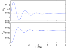
(b) Step response of $x_{1}$ and $x_{2}$

Figure 1: Example of a simple 3 state network

By assuming knowledge of the system order, one may then attempt to fit a state space realization directly from the data. In this case, any attempt to identify a second order system given the oscillating data shown above will result in an $A$ matrix with complex eigenvalues. This implies that any real-valued $A$ matrix that reasonably fits the data will have non-zero terms in its off-diagonal positions, leading incorrectly to a fully connected network structure estimate instead of the correct chain structure.  

II-B Example: Erroneous Structure from Realizations

Suppose that after a sequence of experiments, one was able to identify the transfer function

$$G(s)\left[\begin{array}[]{c}\frac{1}{s+1}\\ \frac{1}{(s+1)(s+2)}\end{array}\right].$$ (6)

It can be shown that this transfer function is consistent with two systems with very different structures, given by

$$A_{1}=\left[\begin{array}[]{rrr}-1&0&0\\ 0&-2&1\\ 0&0&-1\end{array}\right]\ \ B_{1}=\left[\begin{array}[]{c}1\\ 0\\ 1\end{array}\right]\ \ C_{1}=\left[\begin{array}[]{ccc}1&0&0\\ 0&1&0\end{array}\right]$$

and

$$A_{2}=\left[\begin{array}[]{rr}-1&0\\ 1&-2\end{array}\right]\ \ B_{2}=\left[\begin{array}[]{c}1\\ 0\end{array}\right]\ \ C_{2}\left[\begin{array}[]{cc}1&0\\ 0&1\end{array}\right]$$

The networks in Figure 2 correspond to each of the possible realizations of $G$. Note that without more information about the system, such that it is minimal, or order three, etc. then we would not be able to say anything about structure from the transfer function alone.

\psfrag{u}[rt][rt]{$u$}\psfrag{x1}[rt][rt]{$y_{1}$}\psfrag{x2}[rt][rt]{$y_{2}$}\psfrag{x3}[rt][rt]{$x_{3}$}\includegraphics[width=85.35826pt]{figures/ex21a.eps}

(a) Possible network 1.

\psfrag{u}[rt][rt]{$u$}\psfrag{x1}[rt][rt]{$y_{1}$}\psfrag{x2}[rt][rt]{$y_{2}$}\includegraphics[width=85.35826pt]{figures/ex21b.eps}

(b) Possible network 2.

Figure 2: Two possible networks given the data.

These examples demonstrate the difficulty of estimating network structure from data. Nevertheless, ideally one would estimate both the network structure and the system dynamics from data. In the next section, we introduce Dynamical Structure Functions as a mechanism for representing both system dynamics and structure.

III Dynamical Structure

Consider the system given by (1). Given the special structure on $C$, we note that the first p state variables are actually the measured variables $y$. Defining $x_{h}$ to be the remaining $n-p$ “hidden” states, the system becomes

$$\left\{\begin{array}[]{lll}\left[\begin{array}[]{c}\dot{y}\\ \dot{x}_{h}\end{array}\right]&=&\left[\begin{array}[]{cc}A_{11}&A_{12}\\ A_{21}&A_{22}\end{array}\right]\left[\begin{array}[]{c}y\\ x_{h}\end{array}\right]+\left[\begin{array}[]{c}B_{1}\\ B_{2}\end{array}\right]u\\ y&=&\left[\begin{array}[]{cc}I&0\end{array}\right]\left[\begin{array}[]{c}y\\ x_{h}\end{array}\right]\end{array}\right.$$ (7)

Taking Laplace Transforms of the signals, we then obtain

$$\begin{array}[]{lll}\left[\begin{array}[]{c}sY\\ sX_{h}\end{array}\right]&=&\left[\begin{array}[]{cc}A_{11}&A_{12}\\ A_{21}&A_{22}\end{array}\right]\left[\begin{array}[]{c}Y\\ X_{h}\end{array}\right]+\left[\begin{array}[]{c}B_{1}\\ B_{2}\end{array}\right]U\end{array}$$ (8)

From this equation it is easy to construct the transfer functions from the manifest variables $z=[Y\;;\;U]$ to themselves. Solving for $X_{h}$, we have

$$X_{h}=\left(sI-A_{22}\right)^{-1}A_{21}Y+\left(sI-A_{22}\right)^{-1}B_{2}U$$

Substituting into (8) then yields

$$Y=WY+VU$$

where $W=A_{11}+A_{12}\left(sI-A_{22}\right)^{-1}A_{21}$ and $V=A_{12}\left(sI-A_{22}\right)^{-1}B_{2}+B_{1}$. Let $D$ be a matrix with the diagonal term of $W$, i.e. $D=\mbox{diag}(W_{11},W_{22},...,W_{pp})$. Then,

$$\left(sI-D\right)Y=\left(W-D\right)Y+VU$$

Note that $W-D$ is a matrix with zeros on its diagonal. We then have

$$Y=QY+PU$$ (9)

where

$$Q=\left(sI-D\right)^{-1}\left(W-D\right)$$ (10)

and

$$P=\left(sI-D\right)^{-1}V$$ (11)

The matrix $Q$ is a matrix of transfer functions from $Y_{i}$ to $Y_{j}$, $i\neq j$, or relating each measured signal to all other measured signals (recall that $Q$ is zero on the diagonal). The full transfer matrix from $Y$ to $Y$ thus becomes $Q_{T}=I+Q$. Likewise, the transfer matrix from $U$ to $Y$ is $P$.

We thus can consider the transfer matrix, $N$, relating all manifest variables, $z$, to themselves. This matrix is reminiscent of the structure matrix $S$ given in (4), except that the entries are transfer functions relating variables instead of binary values. this gives us the following definition.

Definition 1

Given the system (1), we define the Dynamical Structure Function or Network, $N$, of the system to be

$$N=\left[\begin{array}[]{cc}I+Q&P\\ 0&I\end{array}\right].$$ (12)

where $Q$ and $P$ are as given in (10) and (11).

When this function is completely characterized by $P$ and $Q$ (when the system is open, that is, $u$ represents completely free inputs unrelated to the measurements $y$), we refer to $(P,Q)$ as the Dynamical Structure of the system. There are a number of properties of the Dynamical Structure Function that makes it useful for the structural analysis of linear systems:

Proposition 1

Given the original realisation (1), every entry $N_{ij}$ is a strictly proper function and unique.

Strict properness follows from the fact that $(sI-D)^{-1}$ (which is strictly proper) is multiplying transfer functions that are at most proper (never improper). This fact is important for the interpretation of $N$ as network structure. The directed edges associated with non-zero entries of this matrix imply causal relations; strict properness of the transfer functions preserve this interpretation. Uniqueness follows by construction of both $Q$ and $P$.

Proposition 2

The transfer function, $G$, of the system (1), is related to Dynamic Structure by

$$G=\left(I-Q\right)^{-1}P.$$ (13)

This fact follows directly from (9) and $Y=GU$ and demonstrates that Dynamic Structure is a factorization of a transfer function into two parts, the output or internal structure, $Q$, and the input or control structure, $P$.

It is now easy to see $N_{ij}=0$ if and only if there is no direct or hidden connection from $z_{j}$ to $z_{i}$. The question is then on how to determine the $p^{2}-p$ and $pm$ transfer functions in $Q$ and $P$, respectively, to determine the Dynamical Structure from data. This structure estimation, or reconstruction problem is addressed next.

IV Dynamical Structure Reconstruction

Assume data is collected from the original system (1) leading to the transfer function in (2) relating $Y=GU$. Here we assume without loss of generality that $G$ is full rank. Otherwise, there would be redundant inputs that could be removed to get a full rank $G$. Replacing $Y=GU$ in equation (9) and noting that the vector $U$ is abitrarely yields

$$(I-Q)G=P$$ (14)

This equation shows that there are more unknowns than equations and that in general Dynamical Structure of the $p$ measurable states cannot be obtained from the $m$ inputs. There are $p^{2}-p$ unknowns in $Q$, corresponding to all of the $Q_{ij}$ which represents the internal Dynamical Structure. Then there are $pm$ unknowns in $P$ which represent the control Dynamical Structure on each measurable state. Thus, all together, there are a total of $p^{2}-p+pm$ unknown but only a total of $pm$ equations so the problem is under determined as we have $p^{2}-p$ degrees of freedom. For instance, setting all $Q_{ij}=0$ (which means no connection between measured states) and $P=G$ is a solution of (14) but probably the wrong one.

This clearly shows that the Dynamical Structure has more information than $G$ and less than the original system (1). Thus, to find the Dynamical Structure from $G$ we need more information. Either in the internal Dynamical Structure (if we know some $Q_{ij}=0$), or on how the control is affecting measurable state (if some $P_{ij}=0$). Next we assume we have no information on the internal Dynamical Structure (i.e. no information on $Q$) and consider the cases where: $m<p$ (there are less inputs than measured states), $m=p$ and $m>p$. Before that, we need the following technical result.

Lemma 1

Rank$(P)=$ rank$(G)$.

Proof:

Since $(I-Q)G=P$, if suffices to show that rank$(I-Q)=p$. It follows that rank$(I-Q)$

$$=\ \ \mbox{rank}\left\{I-\left(sI-D\right)^{-1}\left(A_{11}+A_{12}\left(sI-A_{22}\right)^{-1}A_{21}-D\right)\right\}$$

$$=\ \ \mbox{rank}\left\{sI-D-\left(A_{11}+A_{12}\left(sI-A_{22}\right)^{-1}A_{21}-D\right)\right\}$$

$$=\ \ \mbox{rank}\left\{sI-\left(A_{11}+A_{12}\left(sI-A_{22}\right)^{-1}A_{21}\right)\right\}$$

which has rank $=p$.  

IV-A $m<p$: Less Inputs than Measured States

If $m<p$, i.e. there are less inputs than measured states, and we have no information on the internal Dynamical Structure then the Dynamical Structure cannot be recovered. To see this, note that in the best case scenario $m=p-1$ and we would have $mp=p^{2}-p$ equations. Since there are $p^{2}-p$ unknowns from $Q$ we would need to know $P$ precisely.

The example from section II-B shows how different networks satisfy (14) if $m<p$. There we had two measurable states $p=2$, a single input $m=1$ and $G=(G_{11},G_{21})$ given by (6) . In this case, equation (14) has two equations and four unknowns

$$\left\{\begin{array}[]{lll}G_{11}-Q_{12}G_{21}&=&P_{11}\\ G_{21}-Q_{21}G_{11}&=&P_{21}\end{array}\right.$$ (15)

We must solve for the internal Dynamical Structure ($Q_{12}$ and $Q_{21}$) and the control Dynamical Structure ($P_{11}$ and $P_{21}$). Since there are only two equations, there are two degrees of freedom. A possible solution is to set $Q_{12}=Q_{21}=0$, i.e. no internal connection between $y_{1}$ and $y_{2}$. In that case, $P_{11}=G_{11}$ and $P_{21}=G_{21}$ (Figure 2(a)). Note that $x_{3}$ is playing the role of a hidden state (as $P_{21}$ is second-order) and the system is not controllable (due to the common pole at $-1$), which explains why $G$ is second-order and there are three states. An alternative is to have $P_{21}=0$ (which fixes $Q_{21}=G_{21}/G_{11}$) and $Q_{12}=0$ (which fixes $P_{11}=G_{11}$), which can be seen in Figure 2(b). Note that in this case $P_{11}\not=0$ as that would result in a non-proper $Q_{12}$. These two networks are different and obviously only one can be correct.

IV-B $m=p$: Same number of Inputs than Measured States

Theorem 1

If $m=p$ and we have no information on the internal Dynamical Structure, then the Dynamical Structure can be reconstructed if and only if each input controls a measured state independently, i.e. $P_{ij}=0$ for $i\not=j$. In this case, the zeros of $H=G^{-1}$ of the off diagonal define the internal Dynamical Structure and

$$Q_{ij}=-\frac{H_{ij}}{H_{ii}}\ \ \mbox{and}\ \ P_{ii}=\frac{1}{H_{ii}}$$