Formation of spatial patterns in an epidemic model with constant removal rate of the infectives

Abstract

This paper addresses the question of how population diffusion affects the formation of the spatial patterns in the spatial epidemic model by Turing mechanisms. In particular, we present theoretical analysis to results of the numerical simulations in two dimensions. Moreover, there is a critical value for the system within the linear regime. Below the critical value the spatial patterns are impermanent, whereas above it stationary spot and stripe patterns can coexist over time. We have observed the striking formation of spatial patterns during the evolution, but the isolated ordered spot patterns don’t emerge in the space.

I Introduction

The dynamics of spontaneous spatial pattern formation, first introduced to biology by Turing Turing (1952) five decades ago, has recently been attracting attention in many subfields of biology to describe various phenomena. Non-equilibrium labyrinthine patterns are observed in chemical reaction-diffusion systems with a Turing instability Ouyang and Swinney (1991) and in bistable reaction-diffusion systems Hagberg and Meron (1994); Lee and Swinney (1995). Such dynamic patterns in a two dimensional space have recently been introduced into ecology Levin and Segel (1985); Gandhi et al. (1998, 1999); Sayama et al. (2003); Baurmann (2004). In the past few years, geophysical patterns over a wide range of scales for the vegetation have been presented and studied in the Refs. Gilad et al. (2004); von Hardenberg et al. (2001); Lejeune et al. (2002); Rietkerk et al. (2002); HilleRisLambers et al. (2001) using the Turing mechanisms.

In the epidemiology, one of the central goals of mathematical epidemiology is to predict in populations how diseases transmit in the space. For instance, the SARS epidemic spreads through 12 countries within a few weeks. The classical epidemic SIR model describes the infection and recovery process in terms of three ordinary differential equations for susceptibles (S), infected (I), and recovered (R), which has been studied by many researchers Wang and Ruan (2004); Anderson and May (1991); Earn et al. (2000); Diekmann and Kretzschmar (1991) and the reference cited therein. These systems depend mainly on two parameters, the infection rate and the recovery rate.

A growing body of work reports on the role of spatial patterns on evolutionary processes in the host population structure van Ballegooijen and Boerlijst (2004); Boots and Sasaki (1999); Boots et al. (2004); Johnson and Boerlijst (2002); Rand et al. (1995); Haraguchi and Sasaki (2000); Boots (2000). Recent studies have shown large-scale spatiotemporal patterns in measles Grenfell et al. (2001) and dengue fever (DF) Cummings et al. (2004a); Vecchio et al. (2006). More dramatically the wave is often caused by the diffusion (or invasion) of virus within the populations in a given spatial region, thus generating periodic infection, which has been observed in the occurrence of dengue hemorrhagic fever (DHF) in Thailand Cummings et al. (2004b). Existing theoretical work on pathogen evolution and spatial pattern formation has focused on a model in which local invasion to the susceptible hosts plays a central role Boots and Sasaki (1999); Boots et al. (2004); Boots (2000). Projections of the spatial spread of an epidemic and the interactions of human movement at multiple levels with a response protocol will facilitate the assessment of policy alternatives. Spatially-explicit models are necessary to evaluate the efficacy of movement controls Riley et al. (2003); Eubank et al. (2004). A wide variety of methods have been used for the study of spatially structured epidemics, such as cellular automata Liu et al. (2006); Doran and Laffan (2005); Fuks and Lawniczak (2001), networks Bauch and Galvani (2003); Newman (2002), metapopulations Keeling and Gilligan (2000); Lloyd and Jansen (2004), diffusion equations Caraco et al. (2002); Méndez (1998); Reluga et al. (2006), and integro-differential equations, which are useful tools in the study of geographic epidemic spread. In particular, spatial models can be used to estimate the formation of spatial patterns in large-scale and the transmission velocity of diseases, and in turn guide policy decisions.

This paper addresses how diffusive contacts and diffusive movement affect the formation of spatial patterns in two dimensions. The diffusion term is from the earlier work that tracing back to Fisher and Kolmogorov. Noble applied diffusion theory to the spread of bubonic plague in Europe Noble (1974). Noble’s model relies on the assumptions that disease transmits through interactions between dispersing individuals and infected individuals move in uncorrelated random walks. In light of the Turing theoretical and study of recent spatial models, we investigate the formation of spatial patterns in the spatial SIR model based on the study of non-spatial SIR model with constant removal rate of the infectives Wang and Ruan (2004).

II Model

II.1 Basic model

We consider, as the basic model, the following Susceptible-Infected-Recovery (SIR) model

$$\frac{dS}{dt}=A-dS-\lambda SI,$$ (1a)

$$\frac{dI}{dt}=\lambda SI-(d+\gamma)I-h(I),$$ (1b)

$$\frac{dR}{dt}=\gamma I+h(I)-dR,$$ (1c)

where $S(t)$, $I(t)$, and $R(t)$ denote the numbers of susceptible, infective, and recovered individuals at time $t$, respectively. $A$ is the recruitment rate of the population (such as growth rate of average population size, a recover becomes an susceptible, immigrant and so on), $d$ is the natural death rate of the population, $\gamma$ is the natural recovery rate of the infective individuals, and $\lambda$ is a measure of the transmission efficiency of the disease from susceptibles to infectives. In Eq. (1), $h(I)$ is the removal rate of infective individuals due to the treatment. We suppose that the treated infectives become recovered when they are treated in treatment sites. We also suppose that

$$h(I)=\begin{cases}r,&{\rm for}\quad I>0,\\ 0,&{\rm for}\quad I=0,\end{cases}$$ (2)

where $r>0$ is constant and represents the capacity of treatment for infectives. The detail about model (1) can be found in Ref. Wang and Ruan (2004).

II.2 Spatial model

Next we intend to add the spatial parts. Upto the first approximation, the dispersal of individuals can be taken random, so that Fick’ law holds. This gives the flux terms as

$$\frac{\partial S}{\partial t}=D_{s}\nabla^{2}S,\frac{\partial I}{\partial t}=D_{i}\nabla^{2}I,\frac{\partial R}{\partial t}=D_{r}\nabla^{2}R,$$ (3)

where $\nabla^{2}$ ($\nabla^{2}=\frac{\partial^{2}}{\partial x^{2}}+\frac{\partial^{2}}{\partial y^{2}}$) is the Laplacian operator in Cartesian coordinates. $D_{s}$, $D_{i}$, and $D_{r}$ are the diffusion coefficients of the susceptible, infective, and recovered, respectively. Incorporating spatial terms into Eq. (1), it becomes

$$\frac{\partial S}{\partial t}=A-dS-\lambda SI+D_{s}\nabla^{2}S,$$ (4a)

$$\frac{\partial I}{\partial t}=\lambda SI-(d+\gamma)I-h(I)+D_{i}\nabla^{2}I,$$ (4b)

$$\frac{\partial R}{\partial t}=\gamma I+h(I)-dR+D_{r}\nabla^{2}R.$$ (4c)

Generally, we concern on the susceptible and infective individuals. Moreover the Eqs. (4a) and (4b) are independent of the Eq. (4c) whose dynamic behavior is trivial when $I(t_{0})=0$ for some $t_{0}>0$. So it suffices to consider the Eqs. (5a) and (5b) with $I>0$. Thus, we restrict our attention to the following reduced spatial model

$$\frac{\partial S}{\partial t}=A-dS-\lambda SI+D_{s}\nabla^{2}S,$$ (5a)

$$\frac{\partial I}{\partial t}=\lambda SI-(d+\gamma)I-r+D_{i}\nabla^{2}I.$$ (5b)

It is assumed that all the parameters are positive constants from the biological point of view.

III Theoretical analysis of spatial patterns and Results

To study the mechanism of the formation of spatial patterns, firstly, we analyze the stability criterion of the local system. This can be obtained from the Ref. Wang and Ruan (2004). The system (5) has two positive equilibrium points if $R_{0}>1$ and $0<H<(\sqrt{R_{0}}-1)^{2}$, where $R_{0}=\frac{\lambda A}{d(d+\gamma)}$ and $H=\frac{\lambda r}{d(d+\gamma)}$. The two positive equilibrium points are $E_{1}=(S_{1},I_{1})$ and $E_{2}=(S_{2},I_{2})$, where

$$I_{1} = \frac{d}{2\lambda}(R_{0}-1-H-\sqrt{(R_{0}-1-H)^{2}-4H}),$$

$$S_{1} = A/(d+\lambda I_{1}),$$

$$I_{2} = \frac{d}{2\lambda}(R_{0}-1-H+\sqrt{(R_{0}-1-H)^{2}-4H}),$$

$$S_{2} = A/(d+\lambda I_{2}).$$

Diffusion is often considered a stabilizing process, yet it is the diffusion-induced instability in a homogenous steady state that results in the formation of spatial patterns in a reaction-diffusion system Turing (1952). The stability of any system is expressed by the eigenvalues of the system’s Jacobian Matrix. The stability of the homogenous steady state requires that the eigenvalues have negative real parts. To ensure this negative sign, the trace of the Jacobian matrix must be less than zero at steady state if the determinant is greater than zero.

The Jacobian matrix of system (1) at $(S_{2},I_{2})$ is

$$J_{2}=\left(\begin{array}[]{cc}-d-\lambda I_{2}&-\lambda S_{2}\\ \lambda I_{2}&\lambda S_{2}-d-\gamma\end{array}\right)\;.$$ (8)

From the Ref. Qian and Murray (2001), we easily know that there are the Turing space in the system (5) at point $E_{2}$, but at point $E_{1}$ there is no Turing space.

III.1 Stability of the positive equilibrium point in the spatial model

In contrast to the local model, we employ the spatial model in a two-dimensional (2D) domain, so that the steady-state solutions are 2D functions. Let us now discuss the stability of the positive equilibrium point with respect to perturbations. Turing proves that it is possible for a homogeneous attracting equilibrium to lose stability due to the interaction of diffusion process. To check under what conditions these Turing instabilities occur in the model (5), we test how perturbation of a homogeneous steady-state solution behaves in the long-term limit. Here we choose perturbation functions consisting of the following 2D Fourier modes

$$\hat{s}={\rm exp}((k_{x}x+k_{y}y)i+\delta_{k}t),$$ (9a)

$$\hat{i}={\rm exp}((k_{x}x+k_{y}y)i+\delta_{k}t).$$ (9b)

Since we will work with the linearized form of Eq. (5) and the Fourier modes are orthogonal, it is sufficient to analyze the long-term behavior of an arbitrary Fourier mode.

After substituting $S=S_{2}+\hat{s}$ and $I=I_{2}+\hat{i}$ in Eq. (5), we linearize the diffusion terms of the equations via a Taylor-expansion about the positive equilibrium point $E_{2}(S_{2},I_{2})$ and obtain the characteristic equation

$$(J_{\rm sp}-\delta_{k}\textbf{I})\cdot\left(\begin{array}[]{c}\hat{s}\\ \hat{i}\end{array}\right)=0\;,$$ (12)

with

$$J_{\rm sp}=\left(\begin{array}[]{cc}j_{11}-D_{s}k^{2}&j_{12}\\ j_{21}&j_{22}-D_{i}k^{2}\end{array}\right)\;,$$ (15)

here $j_{11}=-d-\lambda I_{2}$, $j_{12}=-\lambda S_{2}$, $j_{21}=\lambda I_{2}$, and $j_{22}=\lambda S_{2}-d-\gamma$. $k^{2}=k_{x}^{2}+k_{y}^{2}$ and $k$ represents the wave numbers.

To find Turing instabilities we must focus on the stability properties of the attracting positive equilibrium point $E_{2}(S_{2},I_{2})$. The loss of stability occurs if at least one of the eigenvalues of the matrix $J_{\rm sp}-\delta_{k}\textbf{I}$ crosses the imaginary axis. From the Eqs. (12) and (15), we can obtain the characteristic equation

$${\rm det}(J_{\rm sp}-\delta_{k}\textbf{I})=\delta_{k}^{2}-{\rm tr}({J_{\rm sp}})\delta_{k}+{\rm det}(J_{\rm sp})=0,$$ (16)

where ${\rm tr}({J_{\rm sp}})={\rm tr}(J_{2})-(D_{s}+D_{i})k^{2}$ and ${\rm det}(J_{\rm sp})={\rm det}(J_{2})-k^{2}(j_{11}D_{i}+j_{22}D_{s})+k^{4}D_{s}D_{i}$. Taking ${\rm tr}(J_{2})>{\rm tr}({J_{\rm sp}})$ into account, we can obtain that for saddles and attractors (both with respect to the non-spatial model) a change of stability coincides with a change of the sign of ${\rm det}(J_{\rm sp})$.

Doing some calculations we find that a change of the sign of ${\rm det}(J_{\rm sp})$ occurs when $k^{2}$ takes the critical values

$$k^{2}_{-}=\frac{j_{11}D_{i}+j_{22}D_{s}-\sqrt{(j_{11}D_{i}+j_{22}D_{s})^{2}-4D_{s}D_{i}{\rm det}(J_{2})}}{2D_{s}D_{i}},$$ (17a)

$$k^{2}_{+}=\frac{j_{11}D_{i}+j_{22}D_{s}+\sqrt{(j_{11}D_{i}+j_{22}D_{s})^{2}-4D_{s}D_{i}{\rm det}(J_{2})}}{2D_{s}D_{i}}.$$ (17b)

In particular, we have

$${\rm det}(J_{\rm sp})<0\Longleftrightarrow k_{-}^{2}<k^{2}<k_{+}^{2}.$$ (18)

If both $k_{-}^{2}$ and $k_{+}^{2}$ exist and have positive values, they limit the range of instability for a local stable equilibrium. We refer to this range as the Turing Space (or Turing Region, see Fig. 1).

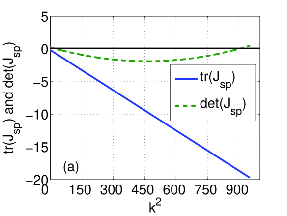
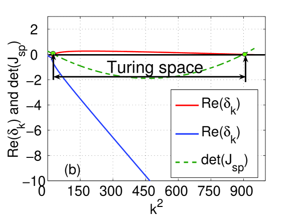
Figure 1: (Color online) This graphes illustrate the eigenvalues of the spatial model (5) at positive equilibrium point $E_{2}(S_{2},I_{2})$, and the loss of stability occurs relation to the limit range wave numbers. (a) For diffusion-driven instability arise both ${\rm tr}(J_{\rm sp})$ and ${\rm det}(J_{\rm sp})$ must be negative for some range of $k^{2}$; (b) The real parts of the eigenvalues of matrix (15) at positive equilibrium $(S_{2},I_{2})$. Model parameters used here are: $A=3$, $d=0.3$, $\lambda=0.35$, $r=0.5$, $\gamma=0.8$, $D_{s}=0.02$, and $D_{i}=0.0005$.

In Fig. 1, the real parts of the eigenvalues of the spatial model (5) at positive equilibrium point $E_{2}(S_{2},I_{2})$ are plotted. From the Eqs. (9a) and (9b), we know that the parameter $\delta_{k}$ can either be a real number or a complex number. If it is a real number, the spatial patterns will emerge and be stable over time and otherwise the spatial patterns will die away quickly. In both case, the sign of the real parts of $\delta_{k}$ (written as $Re(\delta_{k})$) is crucially important to determine whether the patterns will grow or not. In particular if $Re(\delta_{k})>0$, spatial patterns will grow in the linearized system because $|e^{\delta_{k}}|>1$, but if $Re(\delta_{k})<0$ the perturbation decays because $|e^{\delta_{k}}|<1$ and the system returns to the homogeneous steady state. Further details concerning linear stability analysis can be found in Ref. Murray (1993). The Fig. 1 presents the typical situation of Turing instability. With respect to homogenous perturbations, $E_{2}(S_{2},I_{2})$ is stable at first, but when $k^{2}$ increases, one eigenvalue changes its sign (when $k^{2}$ arrives at $k_{-}^{2}$.), the instability occurs. The instability exist until $k^{2}$ reaches $k_{+}^{2}$. When $k^{2}$ is over $k_{+}^{2}$, $(S_{2},I_{2})$ returns stability again. Thus the Turing space is bounded between $k_{-}^{2}$ and $k_{+}^{2}$.

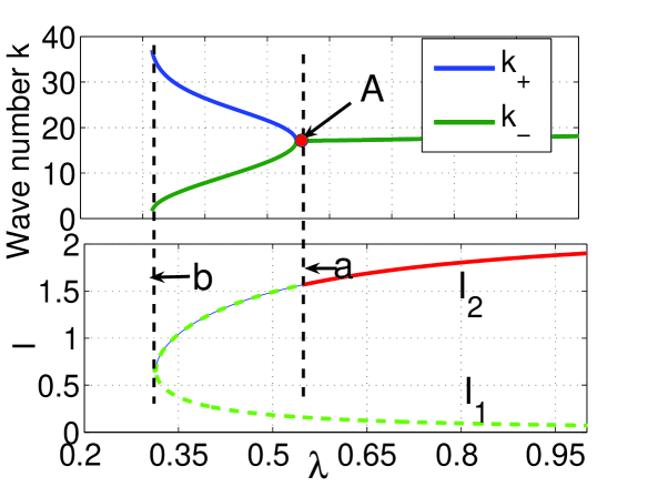
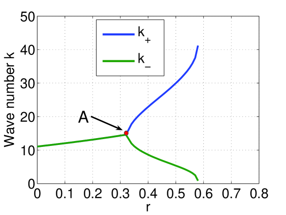
Figure 2: (Color online) The graphes illustrate Turing space versus the parameter $\lambda$ and $r$, respectively. In the Turing space $k_{-}$ and $k_{+}$ curves are shown respectively. (left) The Bifurcation diagrams show the formation of the two stationary solutions of Eq. (5) with fixed $r$ and varying $\lambda$, and values of the parameters are $A=3$, $d=0.3$, $r=0.5$, $\gamma=0.8$, $D_{s}=0.02$, and $D_{i}=0.0005$; In the lower diagram, the green dashed line represents the loss of stability for the positive equilibrium. The red line represents the stable equilibrium. (right) The values of the parameters are $A=3$, $d=0.3$, $\lambda=0.35$, $\gamma=0.8$, $D_{s}=0.02$, and $D_{i}=0.0005$.

The change of the bounds $k_{-}$ and $k_{+}$ with respect to the variation of the $\lambda$ and $r$ are illustrated in the Fig. 2, respectively. The typical feature of Turing space in the model (5) can be observed in Fig. 2. The Turing space is limited by two different bounds. From Fig. 2(left-top) we can see that $k_{-}$ and $k_{+}$ converge in one point A which corresponds to the critical value, $\lambda_{c}$. Beyond right bound (line a), the $E_{2}(S_{2},I_{2})$ exists and is stable. The left bound (line b) of the Turing space shows an “open end”, which corresponds to the saddle-node in the bifurcation plot (see Fig. 2(left-bottom)) for the model (1) and the equilibrium point $E_{2}(S_{2},I_{2})$ does not exist under this bound. This figure shows the solutions of equilibrium points $I_{1}$ and $I_{2}$, where the solid curves represent attractors, dashed curve represents the repellers and saddles, the dotted line a represents the periodic points. This diagram explains the $E_{2}(S_{2},I_{2})$ changes from repeller to attractor, and an unstable orbit of periodical points emerges. From the Fig. 2(right), the curves indicates that $k_{-}$ and $k_{+}$ converge in one point (A). Below that bound, the $E_{2}(S_{2},I_{2})$ exists and is stable. The right bound of the Turing space also shows an “open end”.

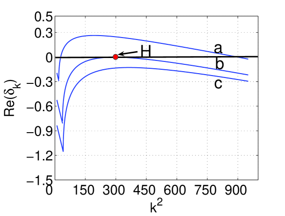
Figure 3: (Color online) Basic dispersion relation giving the growth rate $Re(\delta_{k})$ as a function of the wavenumber $k^{2}$. The mode become marginal at the point (H, $\lambda=\lambda_{c}$) a finite-$k^{2}$ (Turing) mode. The parameter values are $A=3$, $d=0.3$, $r=0.5$, $\gamma=0.8$, $D_{s}=0.02$, and $D_{i}=0.0005$.

Comparing to the two graphes in Fig. 2, one can obtain that the parameters $\lambda$ and $r$ have a similar dynamical behavior in the system for the Turing-bifurcation, but their effects are opposite. We use the parameter $\lambda$ as the Turing-bifurcation parameter in present paper. Fig. 3 shows growth rate curves of the spatial patterns, where at bifurcation (curve b), $\lambda=\lambda_{c}\approx 0.547$ (The threshold $\lambda_{c}$ can be derived analytically, see the Appendix. The analytical and numerical values of $\lambda_{c}$ are approximately equal.), from spatially uniform to spatially heterogenous the critical wave number (point H) is $k_{c}=\sqrt{k_{xc}^{2}+k_{yc}^{2}}$. The curves a and c correspond to the parameter $\lambda=0.35$ below the $\lambda_{c}$, and $\lambda=0.8$ above the $\lambda_{c}$, respectively. The spatial patterns are generated when $\lambda$ passes through the critical Turing-bifurcation point $\lambda_{c}$. And for $\lambda<\lambda_{c}$ there is a finite range of unstable wave numbers which grow exponentially with time, $O({\rm exp}(\delta_{k}t))$, where $\delta_{k}>0$ for a finite range of $k$.

The stable characteristics of $E_{2}(S_{2},I_{2})$ can be changed by the variation of parameter $\lambda$: A sufficiently high increase of $\lambda$ will turns $E_{2}(S_{2},I_{2})$ into an attractor. When changing its characteristics, $E_{2}(S_{2},I_{2})$ traverses a subcritical Hopf bifurcation and an unstable periodic orbit emerges (the dotted line a in Fig. 2(left)). Surprisingly, the latter is not necessarily true, if effect of diffusion comes to play.

III.2 Spatial patterns of the spatial model

The numerical simulations are performed in this section for the spatial model (5) in two dimensions. During the simulation, the periodic boundary conditions are used and part of the parameter values can be determined following Ref. Wang and Ruan (2004) (see the Fig. 1 and 2). We assume that the homogeneous $E_{2}(S_{2},I_{2})$ distributions are in uniform states for each start of the simulation. To induce the dynamics that may lead to the formation of spatial patterns, we perturb the $I$-distribution by small random values.

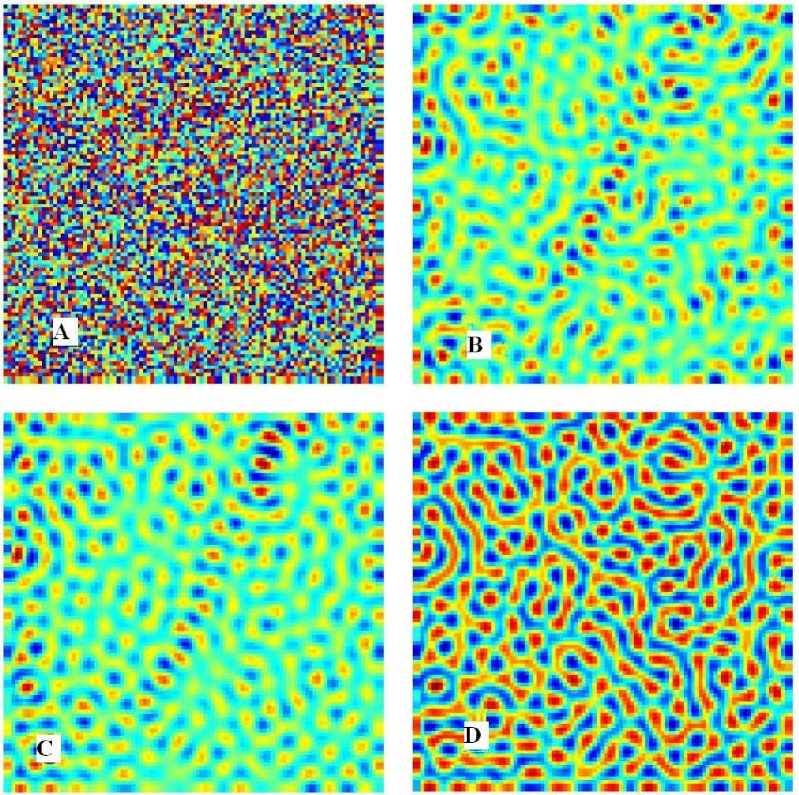
Figure 4: (Color online) Snapshots of contour pictures of the time evolution of $I(x,y,t)$ at different instants. (a)-(c) Numerical results in $100\times 100$ sites. The parameter values are $A=3$, $d=0.3$, $r=0.5$, $\gamma=0.8$, $\lambda=0.65$, $D_{s}=0.02$, $D_{i}=0.0005$, and $\Delta x=\Delta y=0.05$. (A) 0 iteration; (B) 5000 iterations; (C) 30000 iterations; (D) 40000 iterations. [Additional movie formats available from the author]

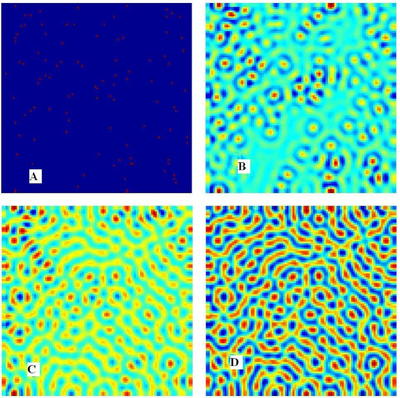
Figure 5: (Color online) Snapshots of contour pictures of the time evolution of $I(x,y,t)$ at different instants. The parameters values are the same as Fig. 4. (A) 0 iteration; (B) 5000 iterations; (C) 40000 iterations; (D) 42000 iterations. [Additional movie formats available from the author]

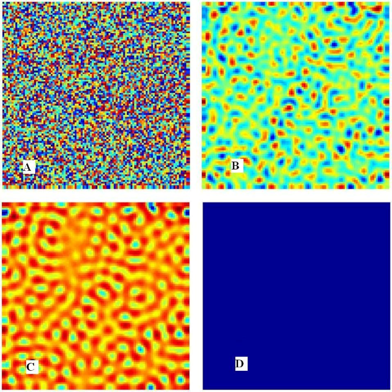
Figure 6: (Color online) Snapshots of contour pictures of the time evolution of $I(x,y,t)$ at different instants. The parameters values are the same as Fig. 4 but $\lambda=0.5$. (A) 0 iteration; (B) 1500 iterations; (C) 8500 iterations; (D) 9400 iterations. [Additional movie formats available from the author]

We study the spatial model (5) by performing stable analysis of the uniform solutions and by integrating Eqs. (5a) and (5b) numerically at different values of $\lambda$ on a grid of $100\times 100$ sites by a simple Euler method with a time step of $\Delta t=0.01$. The results for the infected are summarized below in two dimensions. The model has a uniform free-disease state (no infected) for all constant values of $\lambda$, represented by the solution $S=A/d,I=0$. The free-disease state is stable when $\lambda<\lambda_{c^{\prime}}$. Here $\lambda_{c^{\prime}}$ is a critical value (or threshold ) corresponded by the dotted line b in Fig. 2 (left). Above $\lambda_{c^{\prime}}$ two new states appear, shown in Fig. 2 (left) as line $I_{1}$ and $I_{2}$. The state $I_{2}$ represents a uniformly distributed population with infected density monotonically increasing with $\lambda$. It is instable only for relative values of $\lambda$, $\lambda_{c^{\prime}}<\lambda<\lambda_{c}$ and regains stability when $\lambda>\lambda_{c}$, where the infected density is high. The types of spatial patterns are depended on the range of parameter $\lambda$ as in Figs. 4, 5, and 6. We have made movies of Figs. 4,  5 and  6, respectively, as supplementary materials.

We test several different initial states within the linear regime and the nonlinear regime respectively. Figs. 4 and 5 show that stationary stripe and spot patterns emerge mixtedly in the distribution of the infected population density, where the $\lambda$ is above $\lambda_{c}$ in the linear regime. The initial state of Fig. 4 is the random perturbation of the stable uniform infected state. The initial state of Fig. 5 consists of a few spots (100 scattered spots). Values of the parameters are the same in both two figures. In the linear regime, the result shows that the stripes and spots which describe asymptotic patterns for the spatial model (5) converge at long times. Different initial states may lead to the same type of asymptotic patterns, but the transient behaviors are obviously different (compare the Fig. 4(b) with Fig. 5(b)). Unfortunately, the linear predictions are not accurate in the nonlinear regime.

Fig. 6 shows the snapshots of spatial patterns when the $\lambda$ is between $\lambda_{c^{\prime}}$ and $\lambda_{c}$. One can see that the spatial patterns resemble in Fig. 4 and Fig. 6 at the beginning phase, but differ in the middle and last phases. In Fig. 6, the spatial patterns appear spotted, holed and labyrinthine states in the middle phases, and the spatial patterns appear uniform spatial states in the last phase.

To explain spatial patterns arising from the spatial model, here we present some observations of the spatial and temporal dynamics of dengue hemorrhagic fever epidemics. Dengue fever (DF) is an old disease that became distributed worldwide in the tropics during the 18th and 19th centuries. Fig.7 shows spotted and labyrinth-like spatial patterns of DHF from the field observations Gubler (2002). By comparing the Figs. 4 and 5 with Fig. 7, our results simply capture some key features of the complex variation and explain the observation in spatial structure to most vertebrate species, including humans. In Figs. 4 and 5, the steady spatial patterns indicate the persistence of the epidemic in the space. This result well agrees with the field observation. More examples of the spatial patterns of epidemic, such as HIV, poliovirus, one can find in Refs. Williams et al. (2006); Grassly et al. (2006). In the light of recent work of emphasizing the existence of ‘small world’ networks in human population, our results are also consistent with M. Boots and A. Sasaki’s conclusion that if the world is getting ‘small’–as populations become more connected–disease may evolve higher virulence Boots and Sasaki (1999).

Figure 7: (Color online) Field observations of DHF spatial patters. Reprinted form Trends In Microbiology, Ref. Gubler (2002), Copyright (2002), with permission from Elsevier. Aedes aegypti distribution in the Americas: 1930s, 1970 and 2001.

IV Discussion

In our paper, the labyrinthine patterns are found in the spatial epidemic model driven by the diffusion. The spatial epidemic model comes from the classical non-spatial SIR model which assumes that the epidemic time scale is so tiny related to the demographic time scale that demographic effects may be ignored. But here in the spatial model we take the births and deaths into account. The spatial diffusive epidemic model is more realistic than the classical model. For instance, the history of bubonic plague describes the movement of the disease from place to place carried by rats. The course of an infection usually cannot be modeled accurately without some attention to its spatial spread. To model this would require partial differential equations (PDE), possibly leading to descriptions of population waves analogous to disease waves which have often been observed. Here our spatial model is established from a basic dynamical ‘landscape’ rather than other perturbations, including environmental stochastic variations. From the analysis of the Turing space and numerical simulations one can see that the attracting positive equilibrium will occur instability driven by the diffusion and the instability leads to the labyrinthine patterns within the Turing space. This may explain the prevalence of disease in large-scale geophysics. The positive equilibrium is stable in the non-spatial models, but it may lose its stability with respect to perturbations of certain wave numbers and converge to heterogeneous distributions of populations. It is interesting that we have not observed the isolated spots patterns in the spatial epidemic model (5).

The model (5) is introduced in a general form so that it has broad applications to a range of interacting populations. For example, it can be applied to diseases such as measles, AIDS, flu, etc. Our paper focuses on the deterministic reaction-diffusion equations. However, recent study shows noise plays an important role on the epidemic model Kuske et al. (2007); Dushoff et al. (2004), which indicate that the noise induces sustained oscillations and coherence resonance in the SIR model.

Appendix A Appendixes

Considering the dispersive relation associated with Eqs. (9a) and (9b), the functions of $\delta_{k}$ for the spatial model are defined by the characteristic Eq. (16). Now $Re(\delta_{k})$ predict the unstable wave modes from Eq. (16). One can estimate the most unstable wave number and the critical value of the bifurcation parameter by noticing that at the onset of the instability $\delta_{k}(k_{c})=0$. Thus the constant term in Eq. (16) must be zero at $k_{c}$. In the case of the spatial model this condition is a second order equation on $k_{c}^{2}$, i.e.,

$$D_{s}D_{i}k_{c}^{4}-k_{c}^{2}((-d-\lambda I_{2})D_{i}+(\lambda S_{2}-d-\gamma)D_{s})$$ (19)

$$+(-d-\lambda I_{2})(\lambda S_{2}-d-\gamma)+\lambda^{2}S_{2}I_{2}=0.$$

And as a result the most unstable wave number is given by $\frac{(-d-\lambda I_{2})D_{i}+(\lambda S_{2}-d-\gamma)D_{s}}{2D_{s}D_{i}}$. The critical Turing-bifurcation parameter value, which corresponds to the onset of the instability is defined by Eq. (19). In the spatial model $\lambda$ is the bifurcation parameter adjusting the distance to the onset of the instability. The discriminant of Eq. (19) equals zero for $\lambda_{c}$ and an instability takes place for $\lambda<\lambda_{c}$. Then, we have

$$\lambda_{c} = \frac{(D_{s}S_{2}+D_{i}I_{2}+2\sqrt{D_{s}D_{i}S_{2}I_{2}})(D_{s}\gamma+D_{s}d-D_{i}d)}{(D_{i}I_{2}-D_{s}S_{2})^{2}},$$

where $S_{2}=S_{2}(\lambda_{c})$ and $I_{2}=I_{2}(\lambda_{c})$. We can calculate $\lambda_{c}$ from the Eq. (A) by the computer.

References

- Turing (1952) A. M. Turing, Philos. Trans. R. Soc. London B 237, 7 (1952).
- Ouyang and Swinney (1991) Q. Ouyang and H. L. Swinney, Nature 352, 610 (1991).
- Hagberg and Meron (1994) A. Hagberg and E. Meron, Phys. Rev. Lett. 72, 2494 (1994).
- Lee and Swinney (1995) K. J. Lee and H. L. Swinney, Phys. Rev. E 51, 1899 (1995).
- Levin and Segel (1985) S. A. Levin and L. A. Segel, SIAM Review 27, 45 (1985).
- Gandhi et al. (1998) A. Gandhi, S. Levin, and S. Orszag, J. Theor. Biol. 192, 363 (1998).
- Gandhi et al. (1999) A. Gandhi, S. Levin, and S. Orszag, J. Theor. Biol. 200, 121 (1999).
- Sayama et al. (2003) H. Sayama, M. A. M. de Aguiar, Y. Bar-Yam, and M. Baranger, Forma 18, 19 (2003).
- Baurmann (2004) M. Baurmann, Math. Biosci. and Eng. 1, 111 (2004).
- Gilad et al. (2004) E. Gilad, J. von Hardenberg, A. Provenzale, M. Shachak, and E. Meron, Phys. Rev. Lett. 93, 098105 (2004).
- von Hardenberg et al. (2001) J. von Hardenberg, E. Meron, M. Shachak, and Y. Zarmi, Phys. Rev. Lett. 87, 198101 (2001).
- Lejeune et al. (2002) O. Lejeune, M. Tlidi, and P. Couteron, Phys. Rev. E 66, 010901 (2002).
- Rietkerk et al. (2002) M. Rietkerk, M. C. Boerlijst, F. van Langevelde, R. HilleRisLambers, J. van de Koppel, L. Kumar, H. H. T. Prins, and A. M. de Roos, Am. Nat. 160, 524 (2002).
- HilleRisLambers et al. (2001) R. HilleRisLambers, M. Rietkerk, F. van-den Bosch, H. H. T. Prins, and H. de Kroon, Ecology 82, 50 (2001).
- Wang and Ruan (2004) W. Wang and S. Ruan, J. Math. Anal. Appl. 291, 775 (2004).
- Anderson and May (1991) R. M. Anderson and R. M. May, Infectious Diseases of Humans, Dynamics and control (Oxford University Press, 1991).
- Earn et al. (2000) D. J. D. Earn, P. Rohani, B. M. Bolker, and B. T. Grenfell, Science 287, 667 (2000).
- Diekmann and Kretzschmar (1991) O. Diekmann and M. Kretzschmar, J. Math. Biol. 29, 539 (1991).
- van Ballegooijen and Boerlijst (2004) W. M. van Ballegooijen and M. C. Boerlijst, PNAS 101, 18246 (2004).
- Boots and Sasaki (1999) M. Boots and A. Sasaki, Proc. R. Soc. B 266, 1933 (1999).
- Boots et al. (2004) M. Boots, P. J. Hudson, and A. Sasaki, Science 303, 842 (2004).
- Johnson and Boerlijst (2002) C. R. Johnson and M. C. Boerlijst, Trends. Ecol. & Evol. 17, 83 (2002).
- Rand et al. (1995) D. A. Rand, M. Keeling, and H. B. Wilson, Proc. R. Soc. B 259, 55 (1995).
- Haraguchi and Sasaki (2000) Y. Haraguchi and A. Sasaki, J. Theor. Biol. 203, 85 (2000).
- Boots (2000) Boots, Ecology Letters 3, 181 (2000).
- Grenfell et al. (2001) B. T. Grenfell, O. N. Bjornstad, and J. Kappey, Nature 414, 716 (2001).
- Cummings et al. (2004a) D. A. Cummings, R. A. Irizarry, N. E. Huang, T. P. Endy, A. Nisalak, K. Ungchusak, and D. S. Burke, Nature 427, 344 (2004a).
- Vecchio et al. (2006) A. Vecchio, L. Primavera, and V. Carbone, Phys. Rev. E 73, 031913 (2006).
- Cummings et al. (2004b) D. A. T. Cummings, R. A. Irizarry, N. E. Huang, T. P. Endy, A. Nisalak, K. Ungchusak, and D. S. Burke, Nature 427, 344 (2004b).
- Riley et al. (2003) S. Riley, C. Fraser, C. A. Donnelly, A. C. Ghani, L. J. Abu-Raddad, A. J. Hedley, G. M. Leung, L.-M. Ho, T.-H. Lam, T. Q. Thach, et al., Science 300, 1961 (2003).
- Eubank et al. (2004) S. Eubank, H. Guclu, V. S. Kumar, M. V. Marathe, A. Srinivasan, Z. Toroczkai, and N. Wang, Natrue 429, 180 (2004).
- Liu et al. (2006) Q.-X. Liu, Z. Jin, and M.-X. Liu, Phys. Rev. E 74, 031110 (2006).
- Doran and Laffan (2005) R. J. Doran and S. W. Laffan, Prev. Vet. Med. 70, 133 (2005).
- Fuks and Lawniczak (2001) H. Fuks and A. T. Lawniczak, Discrete Dyn. Nat. Soc. 6, 191 (2001).
- Bauch and Galvani (2003) C. T. Bauch and A. P. Galvani, Math. Biosci. 184, 101 (2003).
- Newman (2002) M. E. J. Newman, Phys. Rev. E 66, 016128 (2002).
- Keeling and Gilligan (2000) M. J. Keeling and C. A. Gilligan, Proc. R. Soc. Lond. B 267, 2219 (2000).
- Lloyd and Jansen (2004) A. L. Lloyd and V. A. A. Jansen, Math. Biosci. 188, 1 (2004).
- Caraco et al. (2002) T. Caraco, S. Glavanakov, G. Chen, J. E. Flaherty, T. K. Ohsumi, and B. K. Szymanski, Am. Nat. 160, 348 (2002).
- Méndez (1998) V. m. c. Méndez, Phys. Rev. E 57, 3622 (1998).
- Reluga et al. (2006) T. C. Reluga, J. Medlock, and A. P. Galvani, Bull. Math. Biol. 68, 401 (2006).
- Noble (1974) J. V. Noble, Nature 250, 726 (1974).
- Qian and Murray (2001) H. Qian and J. D. Murray, Appl. Math. Lett. 14, 405 (2001).
- Murray (1993) J. D. Murray, Mathematical Biology, 2en edn, vol. 19 of Biomathematics series (Berlin: Dpringer, 1993).
- Gubler (2002) D. J. Gubler, TRENDS in Microbiology 10, 100 (2002).
- Williams et al. (2006) B. G. Williams, J. O. Lloyd-Smith, E. Gouws, C. Hankins, W. M. Getz, J. Hargrove, I. de Zoysa, C. Dye, and B. Auvert, PLoS Medicine 3, e262 (2006).
- Grassly et al. (2006) N. C. Grassly, C. Fraser, J. Wenger, J. M. Deshpande, R. W. Sutter, D. L. Heymann, and R. B. Aylward, Science 314, 1150 (2006).
- Kuske et al. (2007) R. Kuske, L. F. Gordillo, and P. Greenwood, J. Theor. Biol. in Press (2007).
- Dushoff et al. (2004) J. Dushoff, J. B. Plotkin, S. A. Levin, and D. J. D. Earn, PNAS 101, 16915 (2004).