Modulation of the reaction rate of regulating protein induces large morphological and motional change of amoebic cell

Abstract

Morphologies of moving amoebae are categorized into two types. One is the “neutrophil” type in which the long axis of cell roughly coincides with its moving direction. This type of cell extends a leading edge at the front and retracts a narrow tail at the rear, whose shape has been often drawn as a typical amoeba in textbooks. The other one is the “keratocyte” type with widespread lamellipodia along the front side arc. Short axis of cell in this type roughly coincides with its moving direction. In order to understand what kind of molecular feature causes conversion between two types of morphologies, and how two typical morphologies are maintained, a mathematical model of amoebic cells is developed. This model describes movement of cell and intracellular reactions of activator, inhibitor and actin filaments in a unified way. It is found that the producing rate of activator is a key factor of conversion between two types. This model also explains the observed data that the keratocye type cells tend to rapidly move along a straight line. The neutrophil type cells move along a straight line when the moving velocity is small, but they show fluctuated motions deviating from a line when they move as fast as the keratocye type cells. Efficient energy consumption in the neutrophil type cells is predicted.

1 Introduction

Amoebic cells have been used as model systems to analyze the molecular mechanism of cell locomotion (Pollard, 2003). Chemical or mechanical signals arriving on amoebic cell membrane induce the intracellular signaling cascade, resulting in the activation of Arp2/3 complex to initiate actin polymerization at the front edge of cell (Pollard and Borisy, 2003). Thus elongated actin filament drives protrusion at the cell anterior. Myosin II seems to play roles in the retraction process at the cell posterior (Eddy et al., 2000), and the cell moves forward when protrusion at the front is followed by retraction at the rear. Although those molecular details have begun to be elucidated, there still remain large mysteries on how biochemical reactions drive the coordinated change of morphology.

Morphologies of moving amoebae seem to be categorized into two types. One is the “neutrophil” type in which the long axis of cell roughly coincides with its moving direction. This type of cell extends a leading edge at the front and retracts a narrow tail, whose shape has been often drawn as a typical amoeba in textbooks. The other one is the “keratocyte” type with widespread lamellipodia along the front side arc. Short axis of cell in this type roughly coincides with its moving direction. Fish or amphibian epidermal keratocytes keep their stable half-moon shape during locomotion and rapidly crawl along the relatively straight line. This stability in morphology and motility has allowed detailed investigations on keratocytes (Lee et al., 1993). Although there is further variety in cell shapes depending on the strength and frequency of protrusion and structures of cytoskeltons, we here focus on the difference whether the shape is head-tail long or laterally long and call the former “neutrophil type ” and the latter “keratocyte type ”.

Interesting observations are that changes in a single or a small number of genes can convert cells from the neutrophil type to the keratocyte type: Breast adenocarcinoma cells overexpressing a Cas-family protein showed morphological conversion to the keratocyte type (Fashena et al., 2002). A cell line of human microvascular endothelial cell moved in a keratocyte-like manner (Kiosses et al., 1999; Fischer et al., 2003). An interesting example of conversion is $amiB$-Null Dictyostelium cells whose amiB gene is disrupted. The wild type Dictyostelium cells are representative neutrophil type cells and move toward the aggregation center with repeated dynamical protrusion and retraction when they are starved. The starved amiB^- cells, on the other hand, move unidirectionally with maintaining a half-moon shape (Asano et al., 2004). A role of AmiB in motility has not yet been known but this example clearly showed that the change in a single gene caused distinct conversion of morphology from the neutrophil type to the keratocyte type.

Here, in this paper we ask questions of what kind of molecular feature causes conversion between two types of morphologies, and how two typical morphologies are maintained. In order to answer these questions, theoretical model is necessary to be developed, which can treat motion, sensing, and chemical reactions in a unified way. Such mathematical model of amoeba has been developed by Nishimura and Sasai (2004, 2005a, 2005b), and it has been shown that the time lag between the shape change and the intracellular molecular diffusion induces cell locomotion with “inertia”-like features: The model can explain experimental observations that once cells are boosted in one direction, cells can keep moving forward without chemoattractants (Verkhovsky et al., 1999) or even toward the direction of decreasing chemoattractants (Jeon et al., 2002). It was predicted that in a “centripetal” distribution of chemoattractants cells can show a rotatory motion by keeping fictitious angular momentum (Nishimura and Sasai, 2005b). These fictitious inertia or angular momentum results from the collective dynamics of morphological change and chemical reactions and diffusion. In the present paper we use this model to explain the dramatic change of morphology between the neutrophil type and the keratocyte type.

2 Model

As in fluid or solid mechanics, the movement of an extended object can be modeled with either way of descriptions, the Lagrange description or the Euler description. In the Lagrange description a cell is regarded to be composed of many small pieces and equations of motions of these pieces are considered. What is advantageous in the Lagrange description is the easiness to treat forces and the mechanical balance among them in cell. In the Euler description, on the other hand, the movement of cell is described from the coordinate fixed in space. This description is useful to treat chemical distributions and reactions in cell. In models of amoebae both two descriptions were adopted in a hybrid manner (Bottino et al., 2002; Rubinstein et al., 2005) to treat the force balance and the chemical reactions at the same time. Another way to express amoebae is to solely use the Euler description. In this case phenomenological rules are used instead of treating the force balance in equations of motions (Satyanarayana and Baumgaertner, 2004). The advantage of this approach is the simplicity in modeling, which allows highly efficient simulation of cell movement. We here adopt the Euler description to calculate a large number of trajectories for statistical sampling.

We introduce hexagonal grids that indicate the simulation space. A cellular body is thought of as a set of single connected grids in the grid space. We call these grids “cellular” grids. We call remaining grids in the model space “external” grids. It has been known that the moving cell repeats adhesion and de-adhesion to substratum, suggesting that the cell movement is regulated by a “clutch-like” mechanism (Smilenov et al., 1999). Here, we simply assume that the cellular grids are linked to the substratum by adhesive molecules and do not slide. Although there are complex biochemical pathways to activate and inactivate adhesive molecules such as integrins and associated proteins, we omit modeling these processes for simplicity. In our model conversion of the external grid to the cellular grid and conversion of the cellular grid to the external grid are assumed to represent adhesion and de-adhesion processes, respectively. If a cellular grid connects at least one external grid, we call this grid a “membrane” grid. If a cellular grid is not a membrane grid, we call that grid “cytoplasm” grid. There are three different molecular densities defined in each cellular grid: activator, $A$, inhibitor, $I$, and actin filaments, $F$. In addition, concentration of the external chemical signal accepted by receptors, $S$, is defined at each membrane grid. Activator and inhibitor are regulating proteins. Though the regulating biochemical network has not yet been fully identified, PI3K and PTEN are candidates of proteins working as activator and inhibitor, respectively (Levchenko and Iglesias, 2002). It is known that PI3K phosphorylates PI(4,5)P₂ to PI(3,4,5)P₃, whereas PTEN dephosphrylates PI(3,4,5)P₃ to PI(4,5)P₂, working in an antagonistic way (Iijima et al., 2002).

We use “rule based dynamics” in which several rules are called randomly. The following paragraphs explain those rules.

(1) Kinetics: Both activator and inhibitor are produced by the stimulation of the external signal (Levchenko and Iglesias, 2002). The activator enhances polymerization of actins, whereas the inhibitor suppresses the polymerization. First, this rule selects a grid in the cellular domain randomly. If densities of activator, inhibitor and actin filaments at the selected grid $j$ are expressed as $A_{j}$, $I_{j}$ and $F_{j}$, respectively, those variables are changed obeying the following equations:

$${A^{\prime}_{j}} = A_{j}+\alpha S_{j}-k_{\alpha}A_{j}$$ (1)

$${I^{\prime}_{j}} = I_{j}+\beta S_{j}-k_{\beta}I_{j}$$ (2)

$${F^{\prime}_{j}} = F_{j}+\left\{\begin{array}[]{ll}\gamma-k_{f}F_{j}&(\frac{A_{j}}{I_{j}}>h)\\ -k_{f}F_{j}&(\mbox{otherwise})\end{array}\right.,$$ (5)

where $\alpha$, $\beta$, $\gamma$, $k_{\alpha}$, $k_{\beta}$, $k_{f}$, $\gamma$ and $h$ are constants. $\alpha$ and $\beta$ are the creation rates of activator and inhibitor, respectively, and $\gamma$ is the rate of polymerization of actin filaments. $k_{\alpha}$ and $k_{\beta}$ are the degradation rates of activator and inhibitor, and $k_{f}$ is the de-polymerization rate of actin filaments. Increase in $h$ decreases the possibility of polymerization of actin filaments. $S_{j}$ indicates the concentration of chemoattractants or the strength of the external signal at the $j$th grid. $S_{j}$ is set to zero if the $j$th grid is in cytoplasm.

(2) Diffusion: Only the inhibitor diffuses into the whole cytoplasm (Levchenko and Iglesias, 2002). This rule selects a grid from the whole cellular domain. At the selected $j$th grid and its nearest cellular $l$th grid, $I_{j}$ and $I_{l}$ obey the following equations:

$$I^{\prime}_{j} = I_{j}-DI_{j}$$ (6)

$$I^{\prime}_{l} = I_{l}+\frac{DI_{j}}{n},$$ (7)

where $D$ is the diffusion constant. $n$ is the number of the nearest cellular grids. $D$ should be smaller than 1 by definition. Since activator and actin filaments do not diffuse and the external signal $S_{j}$ is nonzero only at membrane grids, activator and actin filaments distribute around membrane grids.

(3) Keeping the cell: We also give a rule to prevent cell from breaking into pieces. The cellular volume is kept and the cellular surface length is constrained to be as small as possible. This rule randomly selects a grid from the membrane. Then the rule decides either to remove the grid or to add a new cellular grid around the grid. This rule checks the cellular tension by calculating a cost function, $E$, as $E=(V-V_{0})^{2}+cL^{2}$, where $V$ is the total number of cellular grids and $L$ is the total number of membrane grids, and $V_{0}$ and $c$ are constants. $V_{0}$ is the equilibrium number of cellular grids and $c$ is a ”stiffness”-like factor. When $E^{\prime}$ denotes the cost function after a cellular grid is removed or added, we define the probability $P$ as $P=\exp\left(-\frac{E^{\prime}-E}{kT}\right)$, where $kT$ is a constant to control the extent of fluctuation. We generate a random number between 0 and 1 and then compare the number with $P$. If the number is smaller than $P$, we “undo” the event of removing/adding. Note that if “removing” is chosen, the values of $A$, $I$ and $F$ in the removed grid are added into the nearest cellular grid. If “adding” is chosen, the three values are inherited from a randomly selected nearest grids, and three values of the selected nearest grid are reset to zero.

This rule is related to contraction of the rear of the cell. Recent experimental studies have elucidated that interactions among myosin II and actin filaments generate forces to contract the rear. For cellular locomotion, protrusion at the leading edge seems to have a prime role of cellular “decision making” about where the cell should go (Weber, 2006), and the myosin-generated contraction works to weaken the load of protrusion at the leading edge. In this way the rate of contraction may be regulated so that the cell size is kept as constant as possible. We should note that not only the myosin II contraction but also the cellular cortical tension exerted by actin-myosin network is a factor of keeping the cell size, where myosin I seems to contribute to the generation of cortical tension (Dai et al., 1999). Thus, the effects of the rear contraction and the cortial tension could be modeled by imposing the rule of keeping the cell size. Several theoretical studies on cell locomotion explicitly or implicitly assumed the regulation of keeping cell size in their models (Bottino et al., 2002; Rubinstein et al., 2005). Here, we also impose the rule of keeping cell size instead of considering the detailed mechanisms of contraction and cortical tension. This simplification might be partly justified by the experimental data that the shapes of wildtype Dityostelium discoideum does not differ much from those of myosin-II-null mutants even though the exerted mechanical forces are clearly different (Uchida et al., 2003). The amiB and myosin II double nockout mutants are also known to show a keratocyte-like shape as in mutants which only lacks AmiB (Asano et al., 2004).

(4) Cellular domain extension: The rule randomly selects a grid from the membrane. When $F_{j}$ at the selected $j$th grid in the membrane exceeds the threshold $F_{th}$, an external grid in the six nearest grids of the $j$th grid is turned into a cellular grid. $F_{th}$ roughly defines the amounts of actin filaments per a grid. When there are two or more than two external grids around the $j$th grid, a grid is randomly selected. If this grid is referred to as $l$, $F_{l}=F_{j}/2$ and other variables are set to zero. $F^{\prime}_{j}$ equals to $F_{j}/2$ by definition, where the prime indicates the value at the next time step.

(5) Sampling: The event of sampling does not alter the system but the cellular shape, position, and concentrations of molecules are monitored. “One step” of the cellular dynamics is counted when Sampling is called once.

We also give a master rule that randomly selects one of the above rules. Probabilities of selection for rules from (1) to (5) are written as $P_{1}$, $P_{2}$, $P_{3}$,$P_{4}$ and $P_{5}$, respectively with $P_{1}+P_{2}+P_{3}+P_{4}+P_{5}=1$. When the master rule selects one of the five rules, the selected rule is executed. We iterate this process several millions times.

We assume that the length of a grid is approximately 1 $\mu$m, we put the initial shape of the cell to be a circle with 30-grid diameter, and the equilibrium volume is set to be $V_{0}=900$. The effective diffusion constant of the inhibitor is $D_{\mbox{eff}}\equiv(D/6)(1.0\mu\mbox{m})^{2}/\delta t\times(P_{2}/P_{5})/V_{0}$, where $\delta t$ is the time length of one step. By setting $\delta t=0.3$s, $P_{2}=0.8718$, $P_{5}=0.00029$, and $D=0.45$, we have $D_{\mbox{eff}}\approx 0.8\mu\mbox{m}^{2}/s$, which is of the same order of the diffusion constant of membrane proteins (Gamba et al., 2005). Other parameters are set to prevent the actin filament from spreading too broadly along the membrane but to be heterogeneously distributed in response to the anisotropic environmental stimuli (Iijima et al., 2002); $\beta=0.1$, $k_{\alpha}=0.9$, $k_{\beta}=0.02$, $\gamma=4.0$, $k_{f}=0.99$, $h=10.0$, $F_{th}=1.0$, $P_{1}=0.040686$, $P_{3}=0.05812$, $P_{4}=0.02906$, $c=1.2$ and $kT=20$.

The cell locomotion is simulated with two different patterns of the external signal distributions $S_{j}$: One is “linear gradient” $S_{j}=0.0222y_{j}+1$, where $y_{j}$ indicates the position of the $j$th grid along the $y$ direction in the grid space, and the other is the uniform distribution $S_{j}=1.0$. The cell locomotion follows the gradient of the signal distribution in the former case. Even in the uniform signal distribution of the latter case spontaneous polarization and unidirectional movement of cell have been experimentally observed (Wilkinson, 1998). In the present model intracellular fluctuations of activator and inhibitor are amplified by the fluctuation of the cell shape and grow into the spontaneous cellular locomotion, for which we make observation on the relation between motility and morphology.

3 Results

When the parameter $\alpha$, the rate of activator creation, is set to 1, the long axis of the cell shape roughly coincides with the moving direction of the cell (Fig. 1(a)). The external signal is distributed to have the linear gradient. Fig.1(b), (c) and (d) indicate localization of activator, inhibitor and actin filaments, respectively.

Activator accumulating at the membrane is more localized around the front of cell than the rear, whereas inhibitor distribution is biased towards the rear. As a consequence of such localization of activator and inhibitor, actin filaments are created at the front of the cell. These localized patterns are similar to those observed in Dictyostelium discodeum (Iijima et al., 2002), where PI3K and F-actin are biased towards the front, whereas PTEN accumulates at the rear of Dictyostelium, showing that the cell with $\alpha=1$ is the neutrophil type.

When the parameter $\alpha$ is set to 1.6, the shape becomes keratocyte type, that is, the short axis of the cell shape roughly parallels its moving direction (Fig . 2(a)). The external signal in Fig. 2 has the same linear gradient as in Fig. 1. Localization of activator and inhibitor again leads to creation of actin filaments at the front of cell as shown in Fig. 2 (b), (c) and (d). These features agree with the experimental observations of keratocytes (Svitkina et al., 1997; Verkhovsky et al., 1999) and those of the keratocyte-like cells (Asano et al., 2004). Note that the cellular shape with $\alpha=1.0$ or $\alpha=1.6$ in the uniform external signal is almost same as that in Fig. 2.

In order to analyze the cell shape quantitatively, we calculate the direction of ”minor axis” by fitting an ellipse to the the cell shape;

$$(e_{x},e_{y})=\left(\frac{1}{Z}\sum_{i=1}^{N}x_{i0}y_{i0},\frac{1}{Z}\left[\sum_{i=1}^{N}y_{i0}^{2}-M\right]\right),$$ (8)

where $e_{x}$ and $e_{y}$ are $x$ and $y$-components of a vector pointing along the minor axis and $Z$ is the normalization factor to make $e_{x}^{2}+e_{y}^{2}=1$. $(x_{i0},y_{i0})$ is relative position of the $i$th cellular grid measured from the center of mass of the cell. $M$ is calculated as $M=\frac{1}{2}\left(m_{xx}+m_{yy}+\sqrt{(m_{xx}-m_{yy})^{2}+4m_{xy}^{2})}\right)$, where $m_{xx}=\sum_{i=1}^{N}x_{i0}^{2}$, $m_{yy}=\sum_{i=1}^{N}y_{i0}^{2}$ and $m_{xy}=\sum_{i=1}^{N}x_{i0}y_{i0}$.

The cellular velocity $(v_{x}(t_{n}),v_{y}(t_{n}))$ at time $t_{n}$ is calculated as $v_{x}(t_{n})=(g_{x}(t_{n+m})-g_{x}(t_{n}))/m\delta t$ and $v_{y}(t_{n})=(g_{y}(t_{n+m})-g_{y}(t_{n}))/m\delta t$, where $(g_{x}(t_{n}),g_{y}(t_{n}))$ indicates center of mass of the cellular domain at step $t_{n}$, and $\delta t$ is a step length in the simulation. We select an integer $m$ so that $v(t)$ does not pick up the small fluctuation.

Correlation between the axis and the cellular velocity, $C_{r}$, is calculated by $C_{r}=<|v_{x}e_{x}+v_{y}e_{y}|>/\sqrt{(}v_{x}^{2}+v_{y}^{2})>$, where the bracket $<>$ indicates average over both the time interval in each simulation run and runs started with different random seeds. If there is no correlation between velocity and the direction of minor axis, $C_{r}$ should equal to $\frac{1}{2\pi}\int_{0}^{2\pi}\left|{\rm cos}\theta\right|d\theta=2/\pi\sim 0.6366$. Therefore, we define that the cell is keratocyte and neutrophil type if $C_{r}$ is significantly larger and smaller than $0.6366$, respectively. Fig. 3(a) indicates $C_{r}$ as a function of the parameter $\alpha$, which has a minimum around $\alpha=1.0$ and a maximum around $\alpha=1.6$, showing that the cell becomes neutrophil type around $\alpha=1.0$, and becomes keratocyte type around $\alpha=1.6$. Note that $C_{r}$ seems to be closer to $0.6366$ when $\alpha$ is smaller, showing that the correlation vanishes between the cellular shape and the velocity direction. This is because the cellular shape becomes approximately spherical and the cell fluctuates isotropically as $\alpha$ approaches 0.

Fig. 3(b) shows the relationship between the averaged cellular speed $v=<\sqrt{v_{x}^{2}+v_{y}^{2}}>$ and $\alpha$. The peak exists around $\alpha=1.6$, located at the same $\alpha$ at which the correlation $C_{r}$ shows the peak, which implies that the keratocyte type cell runs faster than cells with other value of $\alpha$.

Fast movement, however, should require more amount of chemical energy. Since ATP is consumed in actin polymerization, amount of ATP molecules used or amount of chemical energy required should be proportional to the number of grids, $N_{g}$, created by the fourth rule. Fig. 3(c) shows the relationship between $\alpha$ and $W=<\delta N_{g}/\delta t>$, where $\delta N_{g}$ is the number of grids created by the fourth rule per one simulation step. $W$ gradually increases as $\alpha$ increases. If energy source would be limited and a cell dose not need to rush to its destination, it is efficient for the cell to reduce “energy per unit length”. We estimate “energy per unit length” as follows:

$$E_{ad}=\left<\frac{\sum_{t}\delta N_{g}/\delta t}{v(t)T}\right>,$$ (9)

where $T$ indicates the time interval of each simulation. Fig. 3(d) indicates that there is a minimum of $E_{ad}$ around $\alpha=1.0$, implying that the neutrophil type cell moves most efficiently.

In order to arrive at cell’s destination rapidly, the cell should move as straight as possible. To estimate this straightness we calculate $S_{t}$ by the distance from the start point to the end point divided by the total path length of the trajectory of the center of mass of the cellular domain. $S_{t}$ ranges from 0 to 1 by definition. $S_{t}$ approaches 1 when the trajectory becomes completely straight. Fig. 3(e) shows that in the uniform distribution of the external signal (indicated by a solid line) a peak exists at $\alpha=1.6$, whereas in the linear gradient distribution (dashed line) a flat peak exists from $\alpha=1.2$ to $1.6$. Although there is a slight difference in $S_{t}$ of keratocyte type ($\alpha=1.6$) and $S_{t}$ of neutrophil type ($\alpha=1.0$), straightness of two types seems almost equivalent.

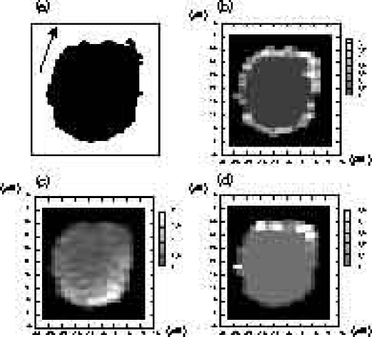
Figure 1: (a) A snapshot of the cell shape with $\alpha=1.0$. An arrow indicates the direction of cellular motion (b) Distribution of activator in the same cell as in (a). Local densities are expressed with gray scale. (c) Distribution of inhibitor. (d) Distribution of actin filaments.

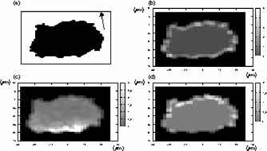
Figure 2: (a) A snapshot of the cell shape with $\alpha=1.6$. (b) Distribution of activator. (c) Distribution of inhibitor. (d) Distribution of actin filaments.

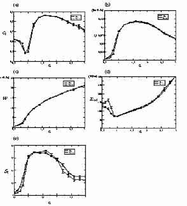
Figure 3: Relationships between the parameter $\alpha$ and five values, $C_{r}$, $v$, $W$, $E_{ad}$ and $S_{t}$. Solid and dashed lines indicate simulations in the environment of the external signal having the linear gradient and the uniform concentration, respectively. The horizontal axis of all graphs is the parameter $\alpha$. (a) The vertical axis is $C_{r}$: correlation between cellular velocity and the semimajor axis of the cell. Error bars indicates standard deviation. All points are values averaged over 50 different simulations started from different random seeds. (b) $v$: Averaged speed. (c) $W$: The number of grids created by the fourth rule per unit time, which is thought to be proportional to the number of consumed ATPs. (d) $E_{ad}$: the number of grids created by the fourth rule per unit length. (e) $S_{t}$: The distance from start point to end point divided by the total path length of the trajectory of the center of mass.

4 Discussion

	$\alpha=0.4$, $\gamma=100$	$\alpha=1.0$, $\gamma=4.0$	$\alpha=1.6$, $\gamma=4.0$
$C_{r}$	$0.51\pm 0.15$	$0.53\pm 0.0065$	$0.86\pm 0.0030$
$v$	$0.11\pm 0.0028$	$0.088\pm 0.001$	$0.12\pm 0.00057$
$W$	$11\pm 0.26$	$6.2\pm 0.068$	$13\pm 0.041$
$E_{ad}$	$97\pm 1.9$	$71\pm 0.39$	$110\pm 0.51$
$S_{t}$	$0.48\pm 0.035$	$0.61\pm 0.0085$	$0.68\pm 0.0064$

Table 1:

Our model shows that the keratocyte type cell moves more rapidly and more straight than other types of cells. These features agree with experimental observations that keratocytes (Lee et al., 1993) or the keratocyte-like $amiB^{-}$ cells (Asano et al., 2004) crawl rapidly along a straight direction. In our model this rapid motion is because of the wide spreading cell membrane at the cell front: Since actin polymerization takes place in the wide area in the keratocyte type cell, the driving force of the forward protrusion is stronger than in the cell with a narrow leading edge.

Another way to realize the rapid motion is to accelerate the polymerization itself. In our model the actin polymerization rate, $\gamma$, controls the rate of actin polymerization. We increase the value of $\gamma$ to 100, meaning that the actin polymerization rate increases twenty-five times. This large change of $\gamma$ is consistent with the fact that the rate of actin polymerization can sensitively vary tens or a hundred times according to the concentrations of G-actin, profin, and other related proteins (Kovar et al., 2006). In order to prevent the cell front from expanding explosively, The creation rate of activator, $\alpha$, is suppressed to be 0.4. Table 1 compares $C_{r}$, $v$, $W$, $E_{ad}$ and $S_{t}$ for three parameter sets with different $\gamma$ and $\alpha$ in the linear gradient condition. The parameter set $(\alpha=0.4,\gamma=100)$ allows the cell to move as fast as the keratocyte type but the motion is less straight. The cell with this parameter set is the neutrophil type having $C_{r}$ value less than $0.6366$; $C_{r}=0.51\pm 0.15$ as summarized in Table 1. Its detailed shape, however, is different from that in Fig. 1(a). Large fluctuation of the cell shape as shown in Fig. 4 is characteristic to this rapidly moving neutrophil type cell, which leads to the less straightforward motion of the cell. Consumed energy is less than the keratocyte type. The wild-type $Dictyostelium$ in the starved phase moves rapidly but along the fluctuating direction and seems to correspond to this type of cell.

Efficient energy usage of the rapidly moving neutrophil type predicted in the model is consistent with the observed decrease in activated NADH in Dictyostelium discodeum cells: Amount of activated NADH should reflect the rate of energy consumption, which is large in unpolrized cells in the vegetative phage but decrases in highly polarized elongated cells in the starved phase (Nomura et al., 2005).

Why does a cell with large $\gamma$ and small $\alpha$ have a fluctuated ”Dicyosteium”-like shape? We can guess the mechanism by following the simulated behavior of cell: Small $\alpha$ suppresses actin polymerization, but once the actin polymerization is initiated as a fluctuation, the large $\gamma$ leads to a rapid protrusion. In this way the large $\gamma$ and small $\alpha$ makes protrusion abrupt and intermittent. This feature of movement of Dicyosteium-like cell gives a sharp contrast to that of the keratocyte type cell. The keratocyte type cell with a larger $\alpha$ but with smaller $\gamma$ shows the continuous actin polymerization, leading to the smooth progression of cell. Thus, the cellular shape and movement decisively depend on $\gamma$ and $\alpha$. Here, we can summarize how the cell shape depends on these two parameters: Small $\gamma$ and small $\alpha$ lead to the slowly moving neutrophil type, small $\gamma$ and large $\alpha$ lead to the keratocyte type, large $\gamma$ and large $\alpha$ lead to the explosive expansion, and large $\gamma$ and small $\alpha$ lead to a Dicyosteium-like shape. It should be interesting to further analyze the morphological change in the two-parameter space of $\gamma$ and $\alpha$ in a quantitative way.

We omitted describing detailed molecular processes of contraction at the rear. Instead, we assumed the rule of keeping cellular size. Although our results showed that this assumption explains several patterns of amoebae, the assumption clearly does not explain the cell locomotion which shows the temporal separation between the protrusion phase and the contraction phase (Uchida et al., 2003). We should improve the model to explicitly take account of the contraction processes, which is left as a further avenue of research.

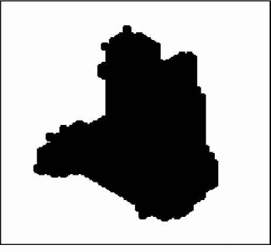
Figure 4: A snapshot of the cell with $\alpha=0.4$ and $\gamma=100$.

5 Conclusion

By using a theoretical model we showed that the rate of production of activator is a key factor to determine whether the cell shape becomes the neutrophil type or the keratocyte type. The apparent morphological conversion between two types can be caused by rather simple biochemical or genetic perturbations which modulate the activator production rate. The keratocyte type cells crawl rapidly along the straight direction by consuming a large amount of energy. Locomotion of the neutrophil type cell is most economic in terms of energy consumption. This slower neutrophil type cell can crawl as straight as the keratocyte type cell. The neutrophil type cell can crawl as rapid as the keratocyte type cell when the rate of actin polymerization is large enough. The moving direction of this rapidly crwaling neutrophil type cell is more fluctuating than the keratocyte type cell. A plausible explanation of the reason why starved $Dictyostelium$ cells take strategy of the rapid neutrophil type locomotion is that they have to gather rapidly but the fine tuning of moving direction with fluctuating trials and errors should be needed when they approach the aggregation center. Further systems biological investigations through simulations with the model which treats the morphological change and chemical reactions in a unified way should enable to classify a variety of different strategies of locomotion and should provide a guide line to design experiments.

References

- Asano et al. (2004) Asano, Y., Mizuno, T., Kon, T., Nagasaki, A., Sutoh, K., Uyeda, T. Q. P., 2004. Keratocyte-like locomotion in amiB-null Dictyostelium cells. Cell Motility and the Cytoskeleton 59, 17–27.
- Bottino et al. (2002) Bottino, D., Mogilner, A., Roberts, T., Stewart, M., Oster, G., 2002. How nematode sperm crawl. Jour. Cell Sci. 115, 367–384.
- Dai et al. (1999) Dai, J., Ting-Beall, H. P., Hochmuth, R. M., Sheetz, M. P., Titius, M. A., 1999. Myosin I contributes to the generation of resting cortical tension. Biophys. Jour. 77, 1168–1176.
- Eddy et al. (2000) Eddy, R. J., Pierini, L. M., Matsumura, F., Maxfield, F. R., 2000. -dependent myosin II activation is required for uropod retraction during neutrophil migration. J. Cell Sci. 113, 1287–1298.
- Fashena et al. (2002) Fashena, S. J., Einarson, M. B., O fNeill, G. M., Patriotis, C., Golemis, E. A., 2002. Dissection of HEF1-dependent functions in motility and transcriptional regulation. J. Cell Biol. 115, 99–111.
- Fischer et al. (2003) Fischer, R. S., Fritz-Six, K. L., Fowler, V. M., 2003. Pointed-end capping by tropomodulin3 negatively regulates endothelial cell motility. J. Cell Biol. 161, 371–380.
- Gamba et al. (2005) Gamba, A., de Candia, A., Talia, S. D., Coniglio, A., Bussolino, F., Serini, G., 2005. Diffusion-limited phase separation in eukaryotic chemotaxis. PNAS 102, 16927–16932.
- Iijima et al. (2002) Iijima, M., Huang, Y. E., Devreotes, P., 2002. Temporal and spatial regulation of chemotaxis. Dev. Cell 3, 469–478.
- Jeon et al. (2002) Jeon, N. L., Baskaran, H., Dertinger, S. K. W., Whitesides, G. M., Water, L. V. D., Toner, M., 2002. Neutrohil chemotaxis in linear and complex gradients of interleukin-8 formed in a microfabricated device. Nat. Biotechnol. 20, 826–830.
- Kiosses et al. (1999) Kiosses, W. B., Daniels, R. H., Otey, C., Bokoch, G. M., Schwartz, M. A., 1999. A role for p21-activated kinase in endothelial cell migration. J. Cell Biol. 147, 831–844.
- Kovar et al. (2006) Kovar, D. R., Harris, E. S., Mahaffy, R., Higgs, H. N., Pollard, T. D., 2006. Control of the assembly of ATP- and ADP-actin by formins and profilin. Cell 124, 423–435.
- Lee et al. (1993) Lee, J., Ishihara, A., Jacobson, K., 1993. Principles of locomotion for simple-shaped cell. Nature 362, 169–171.
- Levchenko and Iglesias (2002) Levchenko, A., Iglesias, P. A., 2002. Models of eukaryotic gradient sensing: Application to chemotaxis of ameobae and neutrophils. Biophys. J. 82, 50–63.
- Nishimura and Sasai (2004) Nishimura, S. I., Sasai, M., 2004. Inertia of chemotactic motion as an emergent property in a model of an eukaryotic cell. In: Proc. of Artificial Life IX. Boston, USA, pp. 410–415.
- Nishimura and Sasai (2005a) Nishimura, S. I., Sasai, M., 2005a. Chemotaxis of an eukaryotic cell in complex gradients of chemoattractants. Artificial Life and Robotics 9, 123–127.
- Nishimura and Sasai (2005b) Nishimura, S. I., Sasai, M., 2005b. Inertia of amoebic cell locomotion as an emergent collective property of the cellular dynamics. Phys. Rev. E E71, 010902 (R) .
- Nomura et al. (2005) Nomura, T., Hidai, C., Nakabayashi, S., 2005. The changes of energy metabolism during the formation of multicellular strcture in Dictyostelium discodeum. Proc. 43th Ann. Meeting of Biophys. Soc. Japan, S179(JAPANESE).
- Pollard (2003) Pollard, T. D., 2003. The cytoskeletion, cellular motility and the reductionist agenda. Nature 422, 741–745.
- Pollard and Borisy (2003) Pollard, T. D., Borisy, G. G., 2003. Cellular motility driven by assembly and disassembly of actin filaments. Cell 112, 453–465.
- Rubinstein et al. (2005) Rubinstein, B., Jacobson, K., Mogilner, A., 2005. Multiscale two-dimensional modeling of a motile simple-shaped cell. Multiscale Model. Simul. 3, 413–439.
- Satyanarayana and Baumgaertner (2004) Satyanarayana, S. V. M., Baumgaertner, A., 2004. Shape and motility of a model cell: A computational study. Jour. Chem. Phys. 121, 4255–4265.
- Smilenov et al. (1999) Smilenov, L. B., Mikhailnov, A., Pelham Jr., R. J., Marcantonio, E. E., Gundersen, G. G., 1999. Focal adhesion motility revealed in stationary fibroblasts. Sci. 286.
- Svitkina et al. (1997) Svitkina, T. M., Verkhovsky, A. B., McQuade, K. M., Borisy, G. G., 1997. Analysis of the actin-myosin II system in fish epidermal keratocytes: Mechanism of cell body translocation. J. Cell. Biol. 139, 397–415.
- Uchida et al. (2003) Uchida, K. S. K., Kitanishi-Yumura, T., Yumura, S., 2003. Myosin II contributes to the posterior contraction and the anterior extension during the retraction phase in migrating Dictyostelium cells. Jour. Cell Sci. 116, 51–60.
- Verkhovsky et al. (1999) Verkhovsky, A. B., Svitkina, T. M., Borisy, G. G., 1999. Self-polarization and directional motility of cytoplasm. Curr. Biol. 9, 11–20.
- Weber (2006) Weber, I., 2006. Is there a pilot in a pseudopod? Eur. Jour. Cell Biol., in press.
- Wilkinson (1998) Wilkinson, P. C., 1998. Assays of leukocyte locomotion and chemotaxis. J. Immunol. Meth. 216, 139–153.