Sea urchin feeding fronts

Abstract

Sea urchin feeding fronts are a striking example of spatial pattern formation in an ecological system. If it is assumed that urchins are asocial, and that they move randomly, then the formation of these dense fronts is an apparent paradox. The key lies in observations that urchins move further in areas where their algal food is less plentiful. This naturally leads to the accumulation of urchins in areas with abundant algae. If urchin movement is represented as a random walk, with a step size that depends on algal concentration, then their movement may be described by a Fokker-Planck diffusion equation. For certain combinations of algal growth and urchin grazing, travelling wave solutions are obtained. Two dimensional simulations of urchin algal dynamics show that an initially uniformly distributed urchin population, grazing on an alga with a smoothly varying density, may form a propagating front separating two sharply delineated regions. On one side of the front algal density is uniformly low, and on the other side of the front algal density is uniformly high. Bounds on when stable fronts will form are obtained in terms of urchin density and grazing, and algal growth.

1 Introduction

Dense, linear aggregations of sea-urchins are sometimes seen. These features, known as feeding-fronts, generally occur at the boundary between grazed and ungrazed habitat (Dean et al., 1984; Scheibling et al., 1999; Alcoverro, 2002; Gagnon et al., 2004). The fronts propagate slowly towards the ungrazed region. Because of the high urchin densities, they are often destructive. A striking example was an aggregation of the urchin Lytechinus variegatus, observed invading sea-grass habitat in Florida Bay (Maciá and Lirman, 1999). The aggregation was estimated to be 2 - 3 m wide and 4 km long, with a density of order 100 urchins m^-2. It is reported to have moved at a rate of up to 6 m day^-1, reducing above-ground seagrass to less than 2% of its initial biomass. Although it became more diffuse with time, the front remained as a coherent feature for at least 10 months. Similar features have been seen in other benthic invertebrates. Linear aggregations of starfish have been recorded invading extensive mussel beds (Dare, 1982), and traveling fronts of strombid conch have also been observed in the Caribbean (Stoner, 1989; Stoner and Lally, 1994) and in Australia (A. MacDiarmid, pers. comm.). Because of the strong influence of such aggregations on the benthic habitat, it is interesting to question how they are formed and maintained.

Herds, flocks, schools, and swarms are all aggregations of social animals. The aggregation is caused by the interaction between the individuals, which attracts them together at large distances (Okubo, 1980). For animals such as sea-urchins there is little evidence that they are social. In uniform habitat their clumping is mild (Andrew and Stocker, 1986; Hagen, 1995). Experiment suggests that urchins will aggregate in the presence of food (Vadas et al., 1986), but there is no evidence for a strong social interaction. Moreover, studies of urchin movement have found that while they may exhibit a chemosensory response to algae, they do not show any directed movement towards it (Andrew and Stocker, 1986). A recent flume tank study shows that the urchin Lytechinus variegatus can move in a directed manner towards a food source under some flow conditions (Pisut, 2002). This may explain how urchins locate their food at short distances. Both the flow and the chemical signals are likely to be more complex in the urchins’ natural environment. In field studies the direction of urchin movement is usually found to be either random or weakly directional (Duggan and Miller, 2001; Dumont et al., 2006; Lauzon-Guay et al., 2006). The question then is how to explain the formation of intense aggregations in an asocial animal, which appears not to be able to move in a directed manner.

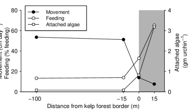
Figure 1: Movement of red sea urchins, Strongylocentrotus franciscanus, near the boundary of a kelp forest at Santa Cruz Point (redrawn from Mattison et al., 1977). The figure shows the average rate of urchin movement, measured over a 24 hour period, at four locations. For comparison, the percentage of urchins which were observed to be feeding, and the weight of algae attached to the urchins’ oral surface, are also shown. Within the kelp forest (shaded), feeding is high and movement rates are low.

A recurrent observation is that there is an inverse relation between urchin movement and macrophyte density (Mattison et al., 1977; Andrew and Stocker, 1986; Dance, 1987; Dumont et al., 2006). A study by Mattison et al. (1977) of red sea-urchins (Strongylocentrotus franciscanus) near Santa Cruz found that urchins within a kelp forest moved by 7.5 cm day^-1, whereas outside it the movement rate increased to over 50 cm day^-1 (Fig. 1). The reasons for the difference in movement rates between habitats is not clear. Some studies find that movement rate is more for starved urchins (Dix, 1970; Hart and Chia, 1990), whereas others find either no effect (Dumont et al., 2006) or the opposite relation (Klinger and Lawrence, 1985). It has also been shown, by using physical models of large algae, that the movement of foliose algae by the water may restrict urchin movement (Konar and Estes, 2003). In this paper, the consequences of differential motility in different habitats will be explored, whatever its cause. Four simple assumptions are made about sea urchin movement:

1. Sea urchins are asocial, with the movements of individual urchins being independent

2. The direction of sea urchin movement is random (over a suitable time period, which we take to be 24 hours)

3. The sea-urchin movement rate decreases as the macrophyte density increases

4. The distance moved in a 24 hour period is related to the seaweed density at the beginning of the time-period.

The consequences of these assumptions are explored, using both analytical techniques and direct simulation. It might seem to be intuitively reasonable that if the urchins are randomly moving then they will disperse, and it will be impossible for them to accumulate into an organised structure like a feeding front. In this paper it is shown that under certain circumstances, and with a suitable representation of macrophyte growth and urchin grazing, the assumptions about urchin movement may lead to persistent urchin feeding fronts.

There are other features of urchin movement which are not accounted for by this model. A recent study (Lauzon-Guay et al., 2006) of sea urchin movement, which followed the movements of individual urchins using video techniques, showed that the distance moved decreased with increasing urchin density. This effect is not included in the present study. Other authors have concluded that the urchin response to predators may mediate the formation of feeding fronts (Bernstein et al., 1981). The model we discuss is a minimal model. The complexities of differential feeding on multi species algal assemblages (Gagnon et al., 2004; Wright et al., 2005), size dependent urchin movement (Dumont et al., 2004, 2006), seasonal variations in movement rate (Konar and Estes, 2001; Dumont et al., 2004), relation between behaviour and the supply of drift algae (Dayton et al., 1984), interactions between movement and the substrate (Laur et al., 1986), or between water movement and urchin movement (Kawamata, 1998) are not included. All demographic processes such as urchin growth, recruitment and mortality have also been ignored. If sufficient data were available these processes could be represented. However, while their inclusion would lead to a more realistic model of a specific system, the purpose of this paper is to explore the consequences of a single urchin behaviour.

2 Urchin movement and the Fokker-Planck equation

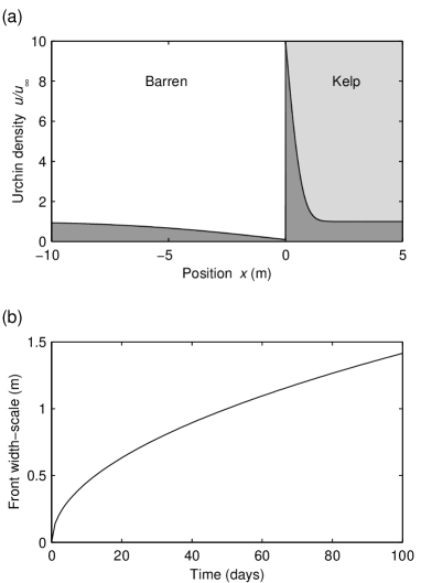
Figure 2: Solution to the Fokker-Planck equation, eq. (2), describing the dispersal of an initially uniform population of sea-urchins in response to a step-change in macrophyte density. The right-hand side, $x>0$, is kelp forest with the urchin movement being $\lambda_{+}=0.1$ m and the left-hand side, $x<0$, is barren with $\lambda_{-}=1$ m (here $\Delta t=1$ day). These values are chosen to be comparable with Mattison et al. (1977). (a) The urchin distribution after 30 days, with the initial population having a value $u/u_{\infty}=1$. There is a net movement of urchins from the barren region to the kelp-forest, with a sharp peak appearing at the kelp boundary. (b) The width of the peak, $2\sqrt{D_{+}t}$, increases very slowly. Even after 100 days it is less than two meters wide. The maximum urchin density is constant with time, at 10 times the initial population.

The four assumptions above may be used to formalize sea-urchin movement as a random walk. If $x_{i}(t)$ is the position of urchin $i$ at time $t$, then its position a time $\Delta t$ later may be represented as

$$x_{i}(t+\Delta t)=x_{i}(t)+\eta(t)\lambda(s(x_{i}(t))),$$ (1)

where $\eta(t)$ is a dimensionless random variable with a zero mean and a unit variance, and $\lambda(s(x))$ (dimensions [$x$]) is a characteristic step-size which is a function of the macrophyte density, $s$.

If the movement of individual sea urchins satisfies eq. (1), then the dispersal of the population may be approximated by the continuous Fokker-Planck equation (Turchin, 1998),

$${\partial u\over\partial t}={\partial^{2}\over\partial x^{2}}(Du),$$ (2)

where $u(x,t)$ is the urchin density and the motility $D(s)$ (dimensions [$x^{2}$ $t^{-1}$]) is related to the random-walk parameters by

$$D(s)={\lambda(s)^{2}\over 2\Delta t}.$$ (3)

The long term behavior of the population $u$ is well-known. If the total number of sea-urchins is constant with time, then the steady state solution to eq. (2) is

$$u(x,t)=c/D(s),$$ (4)

where $c$ is a constant. At equilibrium, the population density will be inversely related to the motility. The sea-urchins will accumulate in areas where the seaweed concentration is higher, and so the individual urchins are moving more slowly. The aggregation of randomly walking foragers in regions with higher food density, is known variously as preytaxis (Kareiva and Odell, 1987), orthokinesis (Okubo, 1980), or phagokinesis (Andrew and Stocker, 1986). An experimental study of ladybugs feeding on an inhomogeneous aphid population showed that, in this case, eq. (4) provided a good description of the data (Turchin, 1998). The random walk formalism is similar to (although simpler than) that used to understand the formation of traveling bands of bacteria through chemotaxis (Keller and Segel, 1971).

While it has been observed that urchin movement is higher when the algal density is lower, little is known about the functional form of $\lambda(s)$. In the absence of any data, we will simply assume that there is a threshold algal density, $s_{c}$, at which the rate of urchin movement changes from a minimum to a maximum value,

$$D=\left\{\begin{array}[]{cl}D_{-},&s<s_{c}\\ D_{+},&s\geq s_{c}\\ \end{array}\right.,$$ (5)

where $D_{-}>D_{+}>0$. Within this model, the urchins have only two behaviours. This simplifying assumption has the advantage of making analytic solutions to the Fokker-Plank equation possible.

3 Analytical solutions

3.1 Solving for a fixed boundary

As a first step towards understanding the formation of feeding-fronts, the response of an urchin population to a step-change in the motility is considered. The boundary between the barren and the kelp regions is assumed to be fixed, with the macrophyte density being greater than the critical density, $s_{c}$, for $x>0$ and less than $s_{c}$ for $x\leq 0$. It follows from eq. (5) that the motility is $D=D_{+}$, ($x>0$) and $D=D_{-}$, ($x\leq 0$), where $D_{\pm}=\lambda^{2}_{\pm}/2\Delta t$. If it is assumed that the urchin population is initially uniformly distributed, then $u(x,0)=u_{\infty}$, where $u_{\infty}$ is a constant.

Away from the boundary between the two regions, the motility is constant and eq. (2) reduces to a diffusion equation. If we write $u(x,t)=u_{+}(x,t)$, ($x\geq 0$) and $u(x,t)=u_{-}(x,t)$, ($x<0$) then, for the derivatives on the right hand side of eq. (2) to be continuous, we require that

$$D_{+}u_{+}(0,t)=D_{-}u_{-}(0,t).$$ (6)

We will look for a solution which has both $u_{+}(0,t)$ and $u_{-}(0,t)$ constant with time, and so will require that $\partial^{2}(Du)/\partial x^{2}|_{x=0}=0$. Because the total urchin population is constant, any increase in the urchin density at positive $x$ must be matched by a decrease in density at negative $x$,

$$\int_{0}^{\infty}(u_{+}-u_{\infty})dx=\int_{-\infty}^{0}(u_{\infty}-u_{-})dx.$$ (7)

The solution to a diffusion equation with a constant boundary is given by the complementary error function,

$$\mathrm{erfc}(x)=1-{1\over\sqrt{\pi}}\int_{0}^{x}e^{-\beta^{2}}d\beta,$$ (8)

with $\beta$ being an integration constant. The solution for the urchin population may be written as

$$u_{\pm}(x,t)=u_{\infty}\left(1\mp\gamma_{\pm}\mathrm{erfc}\left(|x|/2\sqrt{D_{\pm}t}\right)\right),$$ (9)

where $\gamma_{\pm}$ are constants which must satisfy

$$D_{+}\gamma_{+}+D_{-}\gamma_{-}=D_{+}-D_{-}$$ (10)

in order to solve eq. (6). For eq. (7) to hold,

$$\gamma_{+}/\gamma_{-}=\sqrt{D_{-}/D_{+}}.$$ (11)

With this ratio $\partial^{2}Du/\partial x^{2}|_{x=0}=0$, and the Fokker-Planck equation is solved throughout the domain. From eqs. (10) and (11) it follows that

$$\gamma_{\pm}={D_{+}-D_{-}\over\sqrt{D_{\pm}}(\sqrt{D_{-}}+\sqrt{D_{+}})}.$$ (12)

A plot of the solution is given in fig. (2). The initially uniform urchin density develops a peak at the boundary between the two regions. There is an increased urchin density just inside the kelp, and a depleted region on the barren side of the boundary. The height of the peak is constant with time, but the width grows steadily. On the barren side of the peak there is a region where the sea-urchin density is less than the initial value.

3.2 Solving for a moving boundary

We now look for traveling wave solutions of the Fokker-Planck equation, representing a steadily moving urchin front. At this stage, the grazing of the urchins is not considered, it is simply assumed that the boundary between the two regions moves at a constant velocity $c$. The variable $z=x-ct$ is introduced. The traveling solutions are functions of $z$ only, and they satisfy the equation, derived from eq. (2),

$$-c{du\over dz}={d^{2}Du\over dz^{2}},$$ (13)

where $u=u(z)$ and $D=D(z)$. If the boundary between the grazed and ungrazed regions falls at $z=0$, the motility is

$$D(z)=\left\{\begin{array}[]{cl}D_{-},&z\leq 0\\ D_{+},&z>0\\ \end{array}\right..$$ (14)

By integrating eq. (13) twice, an integral equation for the urchin density is obtained,

$$D(z)u(z)=-c\int_{-\infty}^{z}(u(x)-u_{\infty})dx+D_{-}u_{\infty},$$ (15)

where the constant of integration, $u_{\infty}$, has been chosen so that $u(\pm\infty)=u_{\infty}$.

It is straightforward to verify that the solution to eq. (15) is given by the function

$${u(z)\over u_{\infty}}=\left\{\begin{array}[]{ll}1,&z\leq 0\\ {D_{-}-D_{+}\over D_{+}}e^{-cz/D_{+}}+1,&z>0\end{array}\right..$$ (16)

If the motility is larger in the grazed region, $D_{-}>D_{+}$, then the traveling wave solution has the form of a feeding front, with a peak at the boundary between the regions. The maximum density within the feeding front occurs on the boundary, with a density $u_{\infty}D_{-}/D_{+}$. The urchin density is constant throughout the barren region, and decays exponentially towards the ungrazed side of the boundary, the front having a width of $D_{+}/c$.

The feeding front can only propagate continually if there is a non-zero urchin density within the ungrazed region. Otherwise, the front will lose urchins as it travels and decay away.

4 Introducing seaweed

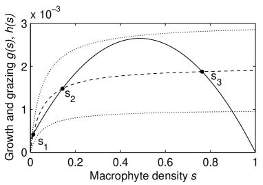
Figure 3: Variation in macrophyte growth $g(s)$ (solid line) and urchin grazing $h(s)$ (dashed line) as a function of the macrophyte density, $s$. The curves follow eqs. (21, 22), with the parameters $\mu_{s}=0.01$ day^-1; $s_{0}=0.03$ $s_{\max}$; $k_{s}=0.05$ $s_{\max}$; $\alpha=0.001$ $s_{\max}$ urchin^-1 day^-1. The dashed line is drawn for an urchin density of $u_{\infty}=2$ urchin m^-2. The three intersection points of $g(s)$ and $h(s)$ are labeled by the macrophyte densities $s_{1}$, $s_{2}$ and $s_{3}$. The upper and lower dotted lines show the urchin grazing with the same parameters, but with urchin densities of $u_{\infty}=3$ urchin m^-2 and $u_{\infty}=1$ urchin m^-2, respectively. With these densities there is only one solution of $ds/dz=0$ (eq. 18), and so there are no possible traveling wave solutions that could represent an urchin feeding-front.

Having identified a frontal solution to the urchin density when the boundary is moving steadily, the question is whether there are traveling wave solutions to the coupled seaweed-urchin equations. The change in algal density is taken to occur through a combination of growth and grazing,

$${\partial s\over\partial t}=g(s)-h(s)u,$$ (17)

where $g(s)$ describes the algal growth and $h(s)u$ is the grazing rate of the urchins on the seaweed. There is no explicit seaweed dispersal included. Recruitment from a wider seaweed population is simply represented by a non-zero intercept of $g(s)$. For a traveling wave solution to exist, $s$ must be a function of $z=x-ct$ only, so

$${\partial s\over\partial z}=h(s)u/c-g(s)/c.$$ (18)

At $z=\pm\infty$ the population must be in equilibrium, $h(s)u_{\infty}=g(s)$, with $s(\infty)>s_{c}$ and $s(-\infty)\leq s_{c}$. There must be at least three real, positive solutions to

$$\partial s/\partial z|_{u=u_{\infty}}=0,$$ (19)

which we shall call $s_{1}$, $s_{2}$, and $s_{3}$ ($s_{3}>s_{2}>s_{1}$). The solutions $s_{1}$ and $s_{3}$ are stable, and $s_{2}$ is unstable. In order that $s<s_{c}$ for $z<0$ it is required that

$$s_{2}>s_{c}>s_{1}.$$ (20)

If this does not hold then no traveling wave solutions can be obtained. The propagation speed can be obtained by requiring that $s=s_{c}$ at $z=0$, where the urchin density, $u$, in eq. (18) is obtained from eq. (16).

As a plausible example, assume that macrophyte growth is logistic

$$g(s)=\mu_{s}(s+s_{0})(1-s/s_{\max}),$$ (21)

where $\mu_{s}$ (dimensions $[t^{-1}]$) is the growth-rate $s_{\max}$(dimensions $[s]$) is the macrophyte carrying capacity and the term $\mu_{s}s_{0}$ (dimensions $[st^{-1}]$) represents a background recruitment rate. With this growth function, the macrophyte will grow to a density $s_{\max}$ in the absence of urchins, and this growth to a maximal density will take a time of order $\mu_{s}^{-1}$.

An appropriate representation of grazing is the Holling type II or Michaelis-Menten equation (Holling, 1959; Begon et al., 1996)

$$h(s)={\alpha s\over s+k_{s}},$$ (22)

where $\alpha$ (dimensions $[su^{-1}t^{-1}]$) parameterizes the maximal grazing rate per urchin, and $k_{s}$ (dimensions $[s]$) is the half-saturation constant for urchin grazing. At low algal densities the grazing function decreases to zero, representing the difficulty that urchins have in locating food when the macrophyte is sparse.

As an example, growth parameters relevant to the New Zealand alga Ecklonia radiata are used. This species grows to a mature size within a year, and so an order-of-magnitude growth-rate is estimated to be $\mu_{s}=0.01$ day^-1. The recruitment density $s_{0}$ will be site specific, depending on the abundance of mature alga in the surrounding area. It is simply assumed that $s_{0}$ is a small fraction of the maximum density, $s_{0}=0.03s_{\max}$. An estimate of urchin grazing rates may be obtained from the results of a small experiment carried out by Russell Cole (1993). A square meter quadrat was loaded with urchins (Evechinus chloroticus), to a density of 60 m^-2, and the decrease in the abundance of the alga E. radiata was monitored. Even at this high urchin density the decline in alga was slow, with a time-scale of $\sim$ 20 days. The maximum grazing rate is therefore $\alpha=1/(20\times 60)=0.001$ $s_{\max}$ urchin^-1 m² day^-1. The algal density at which the urchin grazing is half of its maximum is taken to be $k_{s}=0.1s_{\max}$. In the absence of any data on the variation of urchin motility with algal concentration, it will simply be assumed that the critical algal density is $s_{c}=k_{s}$. The growth and grazing curves that result from these parameters are shown in fig. (3), for three differing urchin densities. Detailed experiment would be needed to verify both the functional form and the parameterization of the growth and grazing functions. The intent here is to illustrate the qualitative features of the urchin-macrophyte system, rather than quantitative modeling of a specific case.

The existence of three solutions to eq. (19) could be determined by directly solving this cubic equation. While analytically tractable, the general solution will be complicated. A more amenable estimate of when three real, positive solutions can be found is readily obtained by graphical inspection of the growth and grazing functions, $g(s)$ and $h(s)$. If the recruitment density $s_{0}$ is zero, then three solutions to eq. (19) will only be found if the initial slope of the grazing function is larger than the initial slope of the growth function. This will only hold if

$$u_{\infty}>{\mu_{s}k_{s}\over\alpha}.$$ (23)

If $k_{s}<<s_{\max}$, then the maximal grazing rate also needs to be less than the maximal growth rate. This implies that

$$u_{\infty}<{\mu_{s}s_{\max}\over 4\alpha}.$$ (24)

Both of these inequalities, (23) and (24), can only be satisfied simultaneously if

$$k_{s}<s_{\max}/4.$$ (25)

If the recruitment density $s_{0}$ is non-zero but small, $s_{0}<<s_{\max}$, then these conditions will still be relevant. For the parameters used in fig. (3) the conditions given in eqs. (23, 24) translate to the requirement that 1 urchin m^-2 $<u_{\infty}<$ 2.5 urchin m^-2. These are not exact bounds, but they provide a useful estimate of the range over which three solutions to eq. (18) can be found.

For a feeding-front solution to exist it is also necessary that the transition from high to low urchin motility occurs at a macrophyte density, $s_{c}$, which is between $s_{1}$ and $s_{2}$ (eq. 20). In the case presented in fig. (3), this would be satisfied by $s_{c}=0.1s_{\max}$. The range of initial urchin densities over which a feeding front solution develops is small, with a factor of less than 3 between a density that leads to macrophyte beds and a density that results in urchin barrens.

5 Numerical simulations

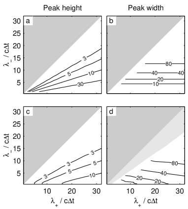
Figure 4: Comparison between the theoretical form of a traveling wave (eq. 16) and numerical simulations, as described in section 5.1. (a) The theoretical peak height, $D_{-}/D_{+}$ (b) The theoretical width, $D_{+}/c$. (c) The maximum height of the peak from the simulations (d) The width of the peak. The half-shading masks the region where the peak height is too small to allow a width to be reliably calculated.

5.1 The traveling wave

For comparison with the analytic solutions numerical simulations are carried out. The first set of simulations aims to check the validity of the traveling wave solution, eq. (16). A one dimensional model is built, which begins with uniformly distributed urchins, each urchin having a real-valued position. The boundary between the low and high motility regions begins at $x=1200$ m and moves towards the right at a velocity $c=1$ m day^-1. At each timestep, for each urchin, a random number $\eta$ is generated from a normal distribution with zero mean and variance. If the urchin is to the right of the boundary it is moved by $\lambda_{+}\eta$. Otherwise, the urchin is moved by $\lambda_{-}\eta$. These rules capture the assumptions which led to the derivation of eq. (16). A window 800 m wide is maintained around the boundary, with a border 150 m wide beyond that. Urchins are added or removed from the simulation to hold the density constant within the two border regions. Any urchins which move beyond the border are removed. The simulation starts with a uniform density of 50 urchins m^-1. It is run for 2000 timesteps, with data from the final 200 timesteps being grouped into 1 m long bins and averaged. The whole simulation is repeated for a range of $\lambda_{+}$ and $\lambda_{-}$ ($\lambda_{-}>\lambda_{+}$). A comparison of the theoretical and the numerical peak widths and heights are shown in fig. (4). There is good agreement between the two approaches, confirming that these simple assumptions can lead to a propagating peak in urchin density.

5.2 Two dimensional simulations with macrophyte

Finally, a simulation is run to check the stability of the feeding fronts in a two-dimensional setting, with macrophyte. A numerical domain is used which represents a 500 m $\times$ 500 m square, divided into 1 m² cells. Each cell has a seaweed density, $s$, with the density going from $s=0$ on the left hand side of the domain to $s=s_{\max}$ on the right hand side. The seaweed distribution has some initial variability, introduced by adding a random function to the linear gradient (fig. 5a). The random function has greater variability at longer length scales, with a Fourier transform that decays as $f^{-3/4}$, where $f$ is the wavenumber. This is done to introduce noise into the model, capturing in some way the natural environmental variability. Urchins are then added, uniformly distributed through the whole domain, and with an average density of 1.5 urchin m^-2. At each timestep the seaweed within each cell changes according to eq. (17). A simple finite-difference approximation is used, and the seaweed density is always kept above zero. The urchin density is calculated from the number of urchins within each 1 m² cell, and the seaweed is grazed accordingly. The urchins are then moved by a random amount, with the size of the step, $\lambda$, depending on whether the seaweed density exceeds the threshold. Any urchins moving outside the domain are reflected back into it, so the total number of urchins within the domain is constant.

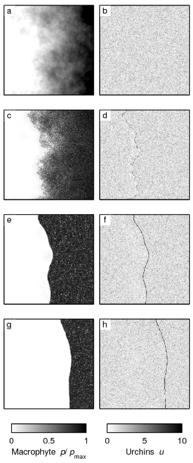
Figure 5: Simulation of seaweed (a, c, e, g) and urchins (b, d, f, h), showing the formation of a feeding front. The pictures are made at 0 (a, b), 600 (c, d), 3000 (e, f) and 6000 (g, h) model days.

The results are shown in fig. (5). In the simulations shown, the following parameters have been used, $\lambda_{+}=0.05$ m day^-1; $\lambda_{-}=1$ m day^-1; $k_{s}=0.05s_{\max}$; $s_{0}=0.01s_{\max}$; $\mu=0.01$ day^-1; $\alpha=0.001s_{\max}$ urchin^-1 m²; and $s_{c}=k_{s}$, similar to the parameters in fig. (3). The simulations are run for 10,000 model days, with the figure showing the seaweed density and the urchin density at 0, 600, 3000 and 6000 model days.

From the start of the simulation the seaweed density becomes increasingly polarized, with areas of urchin barren, and areas of close to maximum density. A feeding front develops along the boundary between the regions, and the boundary slowly propagates towards the ungrazed region. The front appears stable, becoming smoother with time.

6 Discussion

The simple assumptions of differential urchin movement in response to seaweed density lead to the formation and propagation of an urchin feeding front, in qualitative agreement with observations. No social behavior needs to be assumed to explain the persistence of the front, and the motion of each urchin can be random. The system provides an excellent example of how simple individual processes can lead to spatial pattern. The development of the fronts shows the importance of correctly representing movement. Diffusion approximations, based on Fickian diffusion, are often used to represent animal dispersal (Okubo, 1980). Because Fickian diffusion will always lead to the density of a population decreasing (at least in the absence of any reproduction or migration) it is unable to generate sharp fronts. A simple change to the representation of dispersal, from Fickian to Fokker-Planck, leads to a model that captures the qualitative features of the system. The focus of the analysis has been on demonstrating that the system can develop a stable propagating front. This simple model may also be used to explore the dynamics of more transient phenomena, such as the effect of a localised recruitment of urchins, or how a patchy mosaic of barrens and macrophyte habitat can be maintained. With the two states that are stable to small perturbations and the transitional wave transforming one to the other, the urchin-macrophyte system has many of the features of excitable media (Murray, 1993). There is ample scope for further exploration of this analogy.

With the movement rates used here, the propagation speed of the front is very slow. In the two dimensional simulation, the front moved at a speed of 10 m per model year. This is on a similar order to propagation speeds of 2.5 m month^-1 reported from field observations (Gagnon et al., 2004). In contrast the aggregation of Lytechinus variegatus in Florida Bay was reported to move at 6 m day^-1. The propagation rate will be strongly dependent on the details of the urchin grazing. It is likely that the assumption of asociality, or of urchin independence, breaks down at the high densities encountered in the front. Because of the very narrow spatial extent of the frontal region, the urchin behavior at high densities will effect the outcome of the model. To produce a quantitatively accurate model would require more detailed observations. Studies which focus on the movements of individual urchins (Lauzon-Guay et al., 2006) are likely to generate the data required to build a better representation of the frontal dynamics. For example the inclusion of a traffic-jam effect, where the movement rate of the urchins decreases as the density increases (Lauzon-Guay et al., 2006), will result in an increased urchin density within the front.

As discussed in the introduction, there are other processes that are known to influence urchin behaviour which could be represented within a model of this nature. Unfortunately, the effects of many of these factors have only been measured in a few isolated experiments, and there is insufficient published data to include them. The model developed here is in many ways a null model. It is hoped that it will inspire experimentalists to collect the individual based data which is needed to understand the full detail of how urchin feeding fronts are formed and maintained.

7 Acknowledgements

I am grateful to Andrew Visser for discussions on random walks; to Russell Cole for discussions on urchin biology and to Alison MacDiarmid and Alistair Dunn for their support and encouragement. This project was funded by the New Zealand Foundation for Research in Science and Technology.

References

- Alcoverro (2002) Alcoverro, 2002. Effects of sea urchin grazing on seagrass (Thalassodendron ciliatum) beds of a Kenyan lagoon. Mar. Ecol. Prog. Ser. 226, 255–263.
- Andrew and Stocker (1986) Andrew, N. L., Stocker, L. J., 1986. Dispersion and phagokinesis in the echinoid Evechinus chloroticus (Val.). J. Exp. Mar. Biol. Ecol. 100, 11–23.
- Begon et al. (1996) Begon, M., Harper, J. L., Townsend, C. R., 1996. Ecology: Individuals, populations and communities, 3rd Edition. Blackwell Science, Cambridge, MA.
- Bernstein et al. (1981) Bernstein, B. B., Williams, B. E., Mann, K. H., 1981. The role of behavioral responses to predators in modifying urchins’ (Strongylocentrotus droebachiensis) destructive grazing and seasonal foraging patterns. Mar. Biol. 63, 39–49.
- Dance (1987) Dance, C., 1987. Patterns of activity of the sea urchin Paracentrotus lividus in the Bay of Port-Cros (Var, France, Mediterranean). Mar. Ecol. 8, 131–142.
- Dare (1982) Dare, P. J., 1982. Notes on the swarming behaviour and population density of Asterias rubens L. (Echindermata: Asteroidea) feeding on the mussel, Mytilus edulis L. J. Const. int. Explor. Mer. 40, 112–118.
- Dayton et al. (1984) Dayton, P. K., Currie, V., Gerrodette, T., Keller, B. D., Rosenthal, R., Ven Tresca, D., 1984. Patch dynamics and the stability of some California kelp communities. Ecol. Monogr. 54, 253–289.
- Dean et al. (1984) Dean, T. A., Schroeter, S. C., Dixon, J. D., 1984. Effects of grazing by two species of sea urchins (Strongylocentrotus franciscanus and Lytechinus anamesus) on recruitment and survival of two species of kelp (Macrocystis pyrifera and Pterygophora californica). Mar. Biol. 78, 301–313.
- Dix (1970) Dix, T. G., 1970. Biology of Evechinus chloroticus (Echinoidea: Echinometridae) from different localities. N. Z. J. Mar. Freshwat. Res. 4, 267–277.
- Duggan and Miller (2001) Duggan, R. E., Miller, R. J., 2001. External and internal tags for the green sea urchin. J. Exp. Mar. Biol. Ecol. 258, 115–122.
- Dumont et al. (2004) Dumont, C., Himmelman, J. H., Russel, M. P., 2004. Size-specific movement of green sea urchins Strongylocetrotus droebachiensis on urchin barrens in eastern Canada. Mar. Ecol. Prog. Ser. 276, 93–101.
- Dumont et al. (2006) Dumont, C., Himmelman, J. H., Russel, M. P., 2006. Daily movement of the sea urchin Strongylocetrotus droebachiensis in different subtidal habitats in eastern Canada. Mar. Ecol. Prog. Ser. 317, 87–99.
- Gagnon et al. (2004) Gagnon, P., Himmelman, J. H., Johnson, L. E., 2004. Temporal variation in community interfaces: kelp-bed boundary dynamics adjacent to persistent urchin barrens. Mar. Biol. 144, 1191–1203.
- Hagen (1995) Hagen, N. T., 1995. Recurrent destructive grazing of successionally immature kelp forests by green sea urchins in Vestfjorden, Northen Norway. Mar. Ecol. Prog. Ser. 123, 95–106.
- Hart and Chia (1990) Hart, L. J., Chia, F.-S., 1990. Effect of food supply and body size on the foraging behavior of the burrowing sea urchin Echinometra mathaei (de Blainville). J. Exp. Mar. Biol. Ecol. 135, 99–108.
- Holling (1959) Holling, C. S., 1959. Some characteristics of simple types of predation and parasitism. Canadian Entomologist 91, 385–398.
- Kareiva and Odell (1987) Kareiva, P., Odell, G., 1987. Swarms of predators exhibit “preytaxis” if individual predators use area-restricted search. Am. Nat. 130, 233–270.
- Kawamata (1998) Kawamata, S., 1998. Effect of wave-induced oscillatory flow on grazing by a subtidal sea urchin Strongylocentrotus nudus (A. Agassiz). J. Exp. Mar. Biol. Ecol. 224, 31–48.
- Keller and Segel (1971) Keller, E. F., Segel, L. A., 1971. Traveling bands of chemotactic bacteria: a theoretical analysis. J. theor. Biol. 30, 235–248.
- Klinger and Lawrence (1985) Klinger, T. S., Lawrence, J. M., 1985. Distance perception of food and the effect of food quantity on feeding behavior of Lytechinus variegatus (Lamarck) (Echinodermata: Echinoidea). Mar. Behav. Physiol. 11, 327–344.
- Konar and Estes (2001) Konar, B., Estes, J. A., 2001. Seasonal changes in subarctic sea urchin populations from different habitats. Polar Biology 24, 754–763.
- Konar and Estes (2003) Konar, B., Estes, J. A., 2003. The stability of boundary regions between kelp beds and deforested areas. Ecology 84, 174–185.
- Laur et al. (1986) Laur, D. R., Ebeling, A. W., Reed, D. C., 1986. Experimental evaluations of substrate types as barriers to sea urchin (Strongylocentrotus spp.) movement. Mar. Biol. 93, 209–215.
- Lauzon-Guay et al. (2006) Lauzon-Guay, J.-S., Scheibling, R. E., Barbareau, M. A., 2006. Movement patterns in the green sea urchin, Strongylocentrotus droebachiensis. J. Mar. Biol. Ass. U.K. 86, 167–174.
- Maciá and Lirman (1999) Maciá, S., Lirman, D., 1999. Destruction of Florida Bay seagrasses by a grazing front of sea urchins. Bull. Mar. Sci. 65, 593–601.
- Mattison et al. (1977) Mattison, J. E., Trent, J. D., Shanks, A. L., Akin, T. B., Pearse, J. S., 1977. Movement and feeding activity of red sea urchins (Strongylocentrotus francsicanus) adjaceant to a kelp forest. Mar. Biol. 39, 25–30.
- Murray (1993) Murray, J. D., 1993. Mathematical biology, 2nd Edition. Vol. 19 of Biomathematics. Springer-Verlag, Berlin.
- Okubo (1980) Okubo, A., 1980. Diffusion and ecological problems: mathematical models. Vol. 10 of Biomathematics. Springer-Verlag, Berlin.
- Pisut (2002) Pisut, D. P., 2002. The distance chemosensory foraging behavior of the sea urchin Lytechinus variegatus. Master’s thesis, Georgia Institute of Technology, Atlanta, Georgia.
- Scheibling et al. (1999) Scheibling, R. E., Hennigar, A. W., Balch, T., 1999. Destructive grazing, epiphytism, and disease: the dynamics of sea urchin - kelp interactions in Nova Scotia. Can. J. Fish. Aquat. Sci./J. can. sci. halieut. aquat. 56, 2300–2314.
- Stoner (1989) Stoner, A. W., 1989. Winter mass migration of juvenile queen conch Strombus gigas and their influence on the benthic environment. Mar. Ecol. Prog. Ser. 56, 99–104.
- Stoner and Lally (1994) Stoner, A. W., Lally, J., 1994. High-density aggregation in queen conch Strombus gigas: formation, patterns, and ecological significance. Mar. Ecol. Prog. Ser. 106, 73–84.
- Turchin (1998) Turchin, P., 1998. Quantitative analysis of movement. Sinauer, Sunderland.
- Vadas et al. (1986) Vadas, R. L., Elner, R. W., Garwood, P. E., Babb, I. G., 1986. Experimental evaluation of aggregation behavior in the sea urchin Strongylocentrotus droebachiensis. Mar. Biol. 90, 433–448.
- Wright et al. (2005) Wright, J. T., Dworjanyn, S. A., Rogers, C. N., Steinberg, P. D., Williamson, J. E., Poore, A. G. B., 2005. Density-dependent sea urchin grazing : differential removal of species, changes in community composition and alternative community states. Mar. Ecol. 198, 143–156.