A family tree of Markov models
in systems biology

Abstract

Motivated by applications in systems biology, we seek a probabilistic framework based on Markov processes to represent intracellular processes. We review the formal relationships between different stochastic models referred to in the systems biology literature. As part of this review, we present a novel derivation of the differential Chapman-Kolmogorov equation for a general multidimensional Markov process made up of both continuous and jump processes. We start with the definition of a time-derivative for a probability density but place no restrictions on the probability distribution, in particular, we do not assume it to be confined to a region that has a surface (on which the probability is zero). In our derivation, the master equation gives the jump part of the Markov process while the Fokker-Planck equation gives the continuous part. We thereby sketch a “family tree” for stochastic models in systems biology, providing explicit derivations of their formal relationship and clarifying assumptions involved.

Systems Biology and Bioinformatics Group, University of Rostock, A.-Einstein-Str. 21, 18051 Rostock, Germany
^aEmail: mukhtar.ullah@uni-rostock.de
^bEmail: olaf.wolkenhauer@uni-rostock.de, Internet: www.sbi.uni-rostock.de, Tel/Fax: +49 381 498 75 70/72.

Keywords:

Markov processes, stochastic modelling, differential Chapman-Kolmogorov equation, chemical master equations, Fokker-Planck equation, systems biology.

1 Introduction

Systems biology is a merger of systems theory with molecular and cell biology. The key distinguishing feature of a systems biology approach is the description of cell functions (e.g. cell differentiation, proliferation, apoptosis) as dynamic processes [wolkenhauer:05, wolkenhauer:05b, wolkenhauer:05c]. There are two dominant paradigms used in mathematical modelling of biochemical reaction networks (pathways) in systems biology: the “deterministic approach”, using numerical simulations of nonlinear ordinary differential equations (incl. mass action type, power law or Michaelis-Menten models), and the stochastic approach based on master equation and stochastic simulations.

Key references in the area of stochastic modelling are the books by kampen:92, gillespie:92a, breuer:02 and gardiner:04. Most stochastic models presented in these references are derived on the basis of the Chapman-Kolmogorov equation (CKE), a consistency condition on Markov processes, in the form of a system of differential equations for the probability distribution. The system of differential equations take the form of master equations for a jump Markov process and Fokker-Planck equations (FPE) for a continuous Markov process. For the way in which this happens, the reader is referred to [kampen:92] and [gillespie:96, gillespie:92a]. For a Markov process that is made up of both jump and continuous parts, the differential equation takes the form of the differential Chapman-Kolmogorov equation (dCKE) which has been derived in [gardiner:04]. The derivation is involved and requires the introduction of an arbitrary function, which leads to boundary restrictions on the probability distribution. As part of this review, we present a novel and more concise derivation of the dCKE. Since most of the mathematical foundations for stochastic models have been developed by physicists and mathematicians, we hope that our derivation makes the theory more accessible to the uninitiated researcher in the field of systems biology. We choose Markov processes as a framework, since more realistic approaches for modelling intracellular processes must take into account factors such as heterogeneity of the environment, macromolecular crowding [Schnell:04, Ellis:03] and anomalous diffusion [Saxton:94, Saxton:97, Golding:06], to name a few. Anomalous diffusion is described by fractional Fokker-Planck equations [Metzler:00]. Such treatments require advanced mathematical formalisms which are beyond the level assumed in this paper.

The focus of the present paper is neither a comprehensive review of stochastic approaches (See [turner:04] for a recent survey, [paulsson:05, blomberg:06] for a recent theoretical analysis, [rao:02] for a discussion of the role of stochasticity in cell biology) nor a comparison of the two approaches (e.g. [wolkenhauer:04, kummer:05, ullah:06]). Instead, we review the formal relationships between the equations referred to in the systems biology literature. We thereby, try to establish a “family tree” for stochastic models in systems biology, providing explicit derivations of their formal relationship and clarifying assumptions involved in a common framework (See Figure 2). In the following section we focus on the origin of the chemical master equation CME (a special form of the master equation for systems governed by chemical reactions) within the framework of Markov processes. Such generalisation provides a clearer picture of how the various stochastic approaches used in systems biology are related within a common framework.

2 Markov processes

Markov processes form the basis for the vast majority of stochastic models of dynamical systems. The three books by gardiner:04, kampen:92 and gillespie:92a have become standard references for the application of Markov processes to biological and biochemical systems. At the centre of a stochastic analysis is the so-called Chapman-Kolmogorov equation (CKE) that describes the evolution of a Markov process over time. From the CKE stem three equations of practical importance: the master equation for jump-Markov processes, the Fokker-Planck equation (FPE) for continuous Markov processes and the differential Chapman-Kolmogorov equation (dCKE) for processes made up of both the continuous and jump parts. A nice mathematical (but non-biological) account of these equations can also be found in [breuer:02]. Gardiner, van Kampen and Gillespie take different approaches to derive these equations:

• Gillespie derives the FPE and the master equation independently from the CKE and for the one-dimensional case only in [gillespie:92a]. In [gillespie:92, gillespie:96] he extends the derivations to multidimensional cases.

• kampen:92 derives the master equation from the CKE for a one-dimensional Markov process. The FPE is given as an approximation of the master equation by approximating a jump processes with a continuous one. The same approach is adopted in [breuer:02]. However, this should not mislead the reader to conclude that the FPE arises this way. In fact, FPE is defined for a continuous Markov process.

• gardiner:04 derives first the dCKE from the CKE for a multidimensional Markov process whose probability distribution is assumed to be contained in a closed surface. The FPE and the master equation are given as special cases of the dCKE.

We start with a review of basic concepts from probability theory required to read our proof. This is followed by a brief derivation of the CKE and its graphical interpretation. From the CKE we derive the dCKE and interpret its terms to show how the FPE and the master equation appear as special cases of the dCKE. Finally we show that the CME is just a special form of the master equation for jump processes governed by chemical reactions.

A random variable $X$ describes a random event by assigning it values $x$ (called states) from a set $S$ (called state-space) and defines a probability distribution over this set. The set $S$ may be discrete, continuous or both. The probability distribution, in the case of a discrete state-space $S=\left\{n\right\}$, is given by a set of probabilities $p_{n}$ such that

$$\mbox{Prob}\left\{X=n\right\}=p_{n}\,.$$

In the case of a continuous state-space $S=\left\{x\right\}$, the probability distribution is given by a non-negative function $p(x)$ such that

$$\mbox{Prob}\left\{x\leq X<x+dx\right\}=p(x)dx\,.$$

In the literature, $p_{n}$ is referred to as a probability mass function (p.m.f) and $p(x)$ as a probability density function (p.d.f). The delta function $\delta(x)$ defined by

$$\intop_{S}dx\,f(x)\delta(x-c)=f(c)$$ (1)

for any function $f$ of $x$, allows us to write the discrete distribution as a special case of the continuous case. Specifically we write

$$p(x)=\sum_{n}p_{n}\delta(x-n)$$

and note that

$$\mbox{Prob}\left\{X=n\right\}=\intop_{x\leq n<x+dx}dx\,p(x)=\intop_{x\leq n<x+dx}dx\,\sum_{m}p_{m}\delta(x-m)=p_{n}$$

which is what we would expect in the discrete distribution. Since the discrete distribution can always be derived easily from a continuous one, we use hereafter the latter. When dealing with dynamical systems, the probability distribution evolves over time. This leads to the notion of a stochastic process, that is, a system in which random variables are functions of time, written as $X(t)$. The states are scalars for a one-dimensional system and vectors for a multidimensional system. Note that, while the derivations of the master equation and the Fokker-Planck equation in [gillespie:92a, kampen:92] are for the one-dimensional case only, we here present a general treatment and derive all our results for multidimensional systems.

The probability distribution for an $N$-dimensional stochastic process

$$\mathbf{X}(t)=\left(X_{1}(t),\ldots,X_{N}(t)\right)$$

is written as

$$\textup{Prob}\left\{\bigcap_{i=1}^{N}x_{i}\leq X_{i}(t)<x_{i}+dx_{i}\right\}=p(x_{1},\ldots,x_{N},t)dx_{1}\cdots dx_{N}\,.$$

To simplify the notation, we use a short form

$$\textup{Prob}\left\{\mathbf{x}\leq\mathbf{X}(t)<\mathbf{x}+d\mathbf{x}\right\}=p(\mathbf{x},t)d\mathbf{x}\,.$$

More useful will be the conditional probability density, $p(\mathbf{x},t\,|\,\mathbf{x}^{\prime},t^{\prime})$, defined such that

$$\textup{Prob}\left\{\mathbf{x}\leq\mathbf{X}(t)<\mathbf{x}+d\mathbf{x}\,|\,\mathbf{X}(t^{\prime})=\mathbf{x}^{\prime}\right\}=p(\mathbf{x},t\,|\,\mathbf{x}^{\prime},t^{\prime})d\mathbf{x}\,.$$

When $t\geq t^{\prime}$, $p(\mathbf{x},t\,|\,\mathbf{x}^{\prime},t^{\prime})d\mathbf{x}$ is called transition probability. Since it is much easier to work with densities $p(\cdot)$ rather than probabilities $\textup{Prob}\{\cdot\}$, we shall use densities $p(\cdot)$, but abuse the terminology by referring to it as “probabilities”.

Essentially a Markov process is a stochastic process with a short term memory. Mathematically it means that the conditional probability of a state is determined entirely by the knowledge of the most recent state. Specifically for any three successive times $t_{0}\leq t\leq t+\Delta t$ , one has

$$p(\mathbf{x},t+\Delta t\,|\,\mathbf{z},t;\mathbf{x}_{0},t_{0})=p(\mathbf{x},t+\Delta t\,|\,\mathbf{z},t)$$

where the conditional probability of $\mathbf{x}$ at $t+\Delta t$ is uniquely determined by the most recent state $\mathbf{z}$ at $t$ and is not affected by any knowledge of the initial state $\mathbf{x}_{0}$ at $t_{0}$. This Markov property is assumed to hold true for any number of successive time intervals. To see how powerful this property is, let us consider the factorisation of the joint probability

$$p(\mathbf{x},t+\Delta t\,;\,\mathbf{z},t)=p(\mathbf{x},t+\Delta t\,|\,\mathbf{z},t)p(\mathbf{z},t)\,.$$

Making both sides conditional on $(\mathbf{x}_{0},t_{0})$ will modify this equation as

$$p(\mathbf{x},t+\Delta t\,;\,\mathbf{z},t\,|\,\mathbf{x}_{0},t_{0})=p(\mathbf{x},t+\Delta t\,|\,\mathbf{z},t;\mathbf{x}_{0},t_{0})p(\mathbf{z},t\,|\,\mathbf{x}_{0},t_{0})$$

which, by using the Markov property, reduces to

$$p(\mathbf{x},t+\Delta t\,;\,\mathbf{z},t\,|\,\mathbf{x}_{0},t_{0})=p(\mathbf{x},t+\Delta t\,|\,\mathbf{z},t)p(\mathbf{z},t\,|\,\mathbf{x}_{0},t_{0})\,.$$ (2)

The last equation shows that the joint probability can be expressed in terms of transition probabilities. Recall the following rule for joint probabilities

$$p(x)=\int dy\,p(x,y)$$ (3)

which says that summing a joint probability over all values of one of the variables eliminates that variable. Now integrating (2) over $\mathbf{z}$ and using (3), we arrive at the so-called Chapman-Kolmogorov equation (CKE) [gardiner:04]:

$$p(\mathbf{x},t+\Delta t\,|\,\mathbf{x}_{0},t_{0})=\int\limits_{S}d\mathbf{z}\,p(\mathbf{x},t+\Delta t|\mathbf{z},t)p(\mathbf{z},t|\mathbf{x}_{0},t_{0})\,.$$ (4)

This equation expresses the probability of a transition $\left(\mathbf{x}_{0}\rightarrow\mathbf{x}\right)$ as the summation of probabilities of all transitions $\left(\mathbf{x}_{0}\rightarrow\mathbf{z}\rightarrow\mathbf{x}\right)$ via intermediate states $\mathbf{z}$. Figure 1 illustrates the basic notion of a Markov process for which the CKE provides the stochastic formalism. When the initial condition $(\mathbf{x}_{0},t_{0})$ is fixed, which is assumed here, the transition probability conditioned on $(\mathbf{x}_{0},t_{0})$ is the same as the state probability:

$$p(\mathbf{x},t)=p(\mathbf{x},t\,|\,\mathbf{x}_{0},t_{0})\,.$$

Figure 1: Graphical interpretation of the Chapman-Kolmogorov equation. The probability of a transition $\left(\mathbf{x}_{0}\rightarrow\mathbf{x}\right)$ can be obtained by summing probabilities of all transitions $\left(\mathbf{x}_{0}\rightarrow\mathbf{z}\rightarrow\mathbf{x}\right)$, via intermediate states $\mathbf{z}$.

3 Derivation of the dCKE

The CKE serves as a description of a general Markov process, but cannot be used to determine the temporal evolution of the probability. Here we derive from the CKE a differential equation which will be more useful in terms of describing the dynamics of the stochastic process. Referred to as the differential Chapman-Kolmogorov equation (dCKE) by gardiner:04, this equation contains the CME as a special case. This derivation is for a multidimensional Markov process. We start with the definition of a time-derivative for a probability density but place no restrictions on the probability distribution. gardiner:04 instead starts with the expectation of an arbitrary function which results in integration by parts and consequently the need to assume that the probability density vanishes on the surface of a region to which the process is confined. We do not need such as assumption because of the simplicity of our approach. The master equation gives the jump part of the Markov process while the Fokker-Planck equation gives the continuous part.

Consider the time-derivative of the transition probability

$$\frac{\partial}{\partial t}p(\mathbf{x},t)=\lim_{\Delta t\rightarrow 0}\frac{1}{\Delta t}\Bigl{\{}p(\mathbf{x},t+\Delta t)-p(\mathbf{x},t)\Bigr{\}}\,,$$ (5)

where differentiability of the transition probability with respect to time is assumed. Employing the CKE (4) and the normalisation condition

$$\intop_{S}d\mathbf{z}\,p(\mathbf{z},t+\Delta t\,|\,\mathbf{x},t)=1\,,$$

since $p(\mathbf{z},t+\Delta t\,|\,\mathbf{x},t)$ is a probability, (5) can be rewritten as

$$\frac{\partial}{\partial t}p(\mathbf{x},t)=\lim_{\Delta t\rightarrow 0}\frac{1}{\Delta t}\intop_{S}d\mathbf{z}\,\Biggl{\{}p(\mathbf{x},t+\Delta t\,|\,\mathbf{z},t)p(\mathbf{z},t)-p(\mathbf{z},t+\Delta t\,|\,\mathbf{x},t)p(\mathbf{x},t)\Biggr{\}}\,.$$

Let us divide the region $S$ of integration into two regions based on an arbitrarily small parameter $\epsilon>0$. The first region $\left\|\mathbf{x}-\mathbf{z}\right\|<\epsilon$ corresponds to a continuous state process and the above derivative in this region will be denote by $I_{1}$. Here $\left\|\cdot\right\|$ denotes a suitable vector-norm. The second region $\left\|\mathbf{x}-\mathbf{z}\right\|\geq\epsilon$ corresponds to a jump process and the above derivative in this region will be denote by $I_{2}$. Since (6) gives the derivative in the whole region $S$, we can write

$$\frac{\partial}{\partial t}p(\mathbf{x},t)=I_{1}+I_{2},$$ (6)

where

$$I_{1}=\lim_{\Delta t\rightarrow 0}\frac{1}{\Delta t}\intop_{\left\|\mathbf{x}-\mathbf{z}\right\|<\epsilon}d\mathbf{z}\,\Biggl{\{}p(\mathbf{x},t+\Delta t\,|\,\mathbf{z},t)p(\mathbf{z},t)-p(\mathbf{z},t+\Delta t\,|\,\mathbf{x},t)p(\mathbf{x},t)\Biggr{\}},$$

and

$$I_{2}=\lim_{\Delta t\rightarrow 0}\frac{1}{\Delta t}\intop_{\left\|\mathbf{x}-\mathbf{z}\right\|\geq\epsilon}d\mathbf{z}\,\Biggl{\{}p(\mathbf{x},t+\Delta t\,|\,\mathbf{z},t)p(\mathbf{z},t)-p(\mathbf{z},t+\Delta t\,|\,\mathbf{x},t)p(\mathbf{x},t)\Biggr{\}}\,.$$

In the first region $\left\|\mathbf{x}-\mathbf{z}\right\|<\epsilon$, the integrand of $I_{1}$ can be expanded in powers of $\mathbf{x}-\mathbf{z}$ using a Taylor expansion. Setting $\mathbf{x}-\mathbf{z}=\mathbf{r}$, we can write,

$$I_{1}=\lim_{\Delta t\rightarrow 0}\frac{1}{\Delta t}\intop_{\left\|\mathbf{r}\right\|<\epsilon}d\mathbf{r}\,\Biggl{\{}p(\mathbf{x},t+\Delta t\,|\,\mathbf{x}-\mathbf{r},t)p(\mathbf{x}-\mathbf{r},t)-p(\mathbf{x}-\mathbf{r},t+\Delta t\,|\,\mathbf{x},t)p(\mathbf{x},t)\Biggr{\}}\,.$$ (7)

In order to expand the integrand more easily into a Taylor series, let us define a function

$$f(\mathbf{x};\mathbf{r})\triangleq p(\mathbf{x}+\mathbf{r},t+\Delta t\,|\,\mathbf{x},t)p(\mathbf{x},t)$$

so that the integrand in (7) becomes $f(\mathbf{x}-\mathbf{r};\mathbf{r})-f(\mathbf{x};-\mathbf{r})$, which, after a Taylor expansion, becomes

$$-f(\mathbf{x};-\mathbf{r})+f(\mathbf{x};\mathbf{r})+\sum_{i}(-r_{i})\frac{\partial f(\mathbf{x};\mathbf{r})}{\partial x_{i}}+\frac{1}{2}\sum_{i,j}r_{i}r_{j}\frac{\partial^{2}f(\mathbf{x};\mathbf{r})}{\partial x_{i}\partial x_{j}}+\mbox{higher-order terms\,.}$$

The integrals of the first two terms cancel because of the symmetry $\int f(\mathbf{x};\mathbf{r})d\mathbf{r}=\int f(\mathbf{x};-\mathbf{r})d\mathbf{r}$, when the integral is over all the positive and negative values of $\mathbf{r}$ in the region. Thus, we have

$$I_{1}=\lim_{\Delta t\rightarrow 0}\frac{1}{\Delta t}\intop_{\left\|\mathbf{r}\right\|<\epsilon}d\mathbf{r}\,\Biggl{\{}-\sum_{i}r_{i}\frac{\partial}{\partial x_{i}}\Bigl{[}p(\mathbf{x}+\mathbf{r},t+\Delta t\,|\,\mathbf{x},t)p(\mathbf{x},t)\Bigr{]}\\ +\frac{1}{2}\sum_{i,j}r_{i}r_{j}\frac{\partial^{2}}{\partial x_{i}\partial x_{j}}\Bigl{[}p(\mathbf{x}+\mathbf{r},t+\Delta t\,|\,\mathbf{x},t)p(\mathbf{x},t)\Bigr{]}+\mbox{higher-order terms}\Biggr{\}}\,.$$

For the state increments $X_{i}(t+\Delta t)-X_{i}(t)$, recognising the (conditional) expectations

$$\langle X_{i}(t+\Delta t)-X_{i}(t)\,|\,\mathbf{X}(t)=\mathbf{x}\rangle=\intop_{\left\|\mathbf{r}\right\|<\epsilon}d\mathbf{r}\,r_{i}\,p(\mathbf{x}+\mathbf{r},t+\Delta t\,|\,\mathbf{x},t)$$

and

$$\langle\left[X_{i}(t+\Delta t)-X_{i}(t)\right]\left[X_{j}(t+\Delta t)-X_{j}(t)\right]\,|\,\mathbf{X}(t)=\mathbf{x}\rangle\\ =\intop_{\left\|\mathbf{r}\right\|<\epsilon}d\mathbf{r}\,r_{i}r_{j}\,p(\mathbf{x}+\mathbf{r},t+\Delta t\,|\,\mathbf{x},t),$$

we refer to the differentiability conditions for continuous processes, i.e., $\left\|\mathbf{x}-\mathbf{z}\right\|<\epsilon$ [gardiner:04, section 3.4]:

$$\lim_{\Delta t\rightarrow 0}\frac{\langle X_{i}(t+\Delta t)-X_{i}(t)\,|\,\mathbf{X}(t)=\mathbf{x}\rangle}{\Delta t} =A_{i}(\mathbf{x},t)+o(\epsilon)$$ (8)

$$\lim_{\Delta t\rightarrow 0}\frac{\langle\left[X_{i}(t+\Delta t)-X_{i}(t)\right]\left[X_{j}(t+\Delta t)-X_{j}(t)\right]\,|\,\mathbf{X}(t)=\mathbf{x}\rangle}{\Delta t} =B_{ij}(\mathbf{x},t)+o(\epsilon)$$ (9)

where $o(\epsilon)$ represents vanishing terms, such that $\lim_{\epsilon\rightarrow 0}o(\epsilon)/\epsilon=0$. The higher-order terms involve higher-order coefficients which must vanish. To see that, for the third-order coefficient

$$\lim_{\Delta t\rightarrow 0}\frac{1}{\Delta t}\intop_{\left\|\mathbf{r}\right\|<\epsilon}d\mathbf{r}\,r_{i}r_{j}r_{k}\,p(\mathbf{x}+\mathbf{r},t+\Delta t\,|\,\mathbf{x},t)=C_{ijk}(\mathbf{x},t)+o(\epsilon)\,.$$

However

$$\lim_{\Delta t\rightarrow 0}\frac{1}{\Delta t}\intop_{\left\|\mathbf{r}\right\|<\epsilon}d\mathbf{r}\,r_{i}r_{j}r_{k}\,p(\mathbf{x}+\mathbf{r},t+\Delta t\,|\,\mathbf{x},t)$$

$$\leq \left\|\mathbf{r}\right\|\lim_{\Delta t\rightarrow 0}\frac{1}{\Delta t}\intop_{\left\|\mathbf{r}\right\|<\epsilon}d\mathbf{r}\,r_{i}r_{j}\,p(\mathbf{x}+\mathbf{r},t+\Delta t\,|\,\mathbf{x},t)$$

$$\leq \epsilon\left[B_{ij}(\mathbf{x},t)+o(\epsilon)\right]$$

$$\leq o(\epsilon)\,.$$

Hence $C(\mathbf{x},t)$ must vanish. The vanishing of higher-order coefficients follows immediately. In physics, the vector $A(\mathbf{x},t)$ is known as the “drift vector” and the matrix $B(\mathbf{x},t)$ as the “diffusion matrix”. This terminology is suggested by the observation that, given $X(t)=x$, the state increment vector $\mathbf{X}(t+dt)-\mathbf{X}(t)$ for a continuous process has a mean approaching $A(\mathbf{x},t)dt$ and a covariance approaching $B(\mathbf{x},t)dt$, as $\epsilon$ approaches zero. This also suggests the following update rule, for $\epsilon\rightarrow 0$ and under assumptions given in [gardiner:04, section 3.5.2],

$$\mathbf{X}(t+dt)=\mathbf{X}(t)+A(\mathbf{X}(t),t)dt+\left[B(\mathbf{X}(t),t)dt\right]^{1/2}$$ (10)

which is a form of the “Langevin equation” [kampen:92]. We remark here that (8) and (9) are postulated here for mathematical convenience. A more rigorous justification is given in [gillespie:96]. Subject to the differentiability conditions (8) and (9), we see that as $\epsilon\rightarrow 0$,

$$I_{1}\rightarrow-\sum_{i}\frac{\partial}{\partial x_{i}}\Bigl{[}A_{i}(\mathbf{x},t)p(\mathbf{x},t)\Bigr{]}+\frac{1}{2}\sum_{i,j}\frac{\partial^{2}}{\partial x_{i}\partial x_{j}}\Bigl{[}B_{ij}(\mathbf{x},t)p(\mathbf{x},t)\Bigr{]}\,.$$ (11)

Next we work out the jump probability rate

$$I_{2}=\lim_{\Delta t\rightarrow 0}\frac{1}{\Delta t}\intop_{\left\|\mathbf{x}-\mathbf{z}\right\|\geq\epsilon}d\mathbf{z}\,\Biggl{\{}p(\mathbf{x},t+\Delta t\,|\,\mathbf{z},t)p(\mathbf{z},t)-p(\mathbf{z},t+\Delta t\,|\,\mathbf{x},t)p(\mathbf{x},t)\Biggr{\}}\,.$$

We will use the differentiability condition for jump processes, i.e., $\left\|\mathbf{x}-\mathbf{z}\right\|\geq\epsilon$ [gardiner:04, section 3.4]:

$$\lim_{\Delta t\rightarrow 0}\frac{1}{\Delta t}p(\mathbf{x},t+\Delta t\,|\,\mathbf{z},t)=W(\mathbf{x}\,|\,\mathbf{z},t)\,,$$

where $W(\mathbf{x}\,|\,\mathbf{z},t)$ is called the transition rate for the jump $(\mathbf{z}\rightarrow\mathbf{x})$. Subject to this condition, we see that as $\epsilon\rightarrow 0$, the region of integration approaches $S$, leading to

$$I_{2}\rightarrow\intop_{S}d\mathbf{z}\,\Bigl{[}W(\mathbf{x}\,|\,\mathbf{z},t)p(\mathbf{z},t)-W(\mathbf{z}\,|\,\mathbf{x},t)p(\mathbf{x},t)\Bigr{]}\,.$$ (12)

Adding (11) and (12), we can rewrite (6) to arrive at the dCKE:

$$\frac{\partial}{\partial t}p(\mathbf{x},t)=-\sum_{i}\frac{\partial}{\partial x_{i}}\Bigl{[}A_{i}(\mathbf{x},t)p(\mathbf{x},t)\Bigr{]}+\frac{1}{2}\sum_{i,j}\frac{\partial^{2}}{\partial x_{i}\partial x_{j}}\Bigl{[}B_{ij}(\mathbf{x},t)p(\mathbf{x},t)\Bigr{]}\\ +\intop_{S}d\mathbf{z}\,\Bigl{[}W(\mathbf{x}\,|\,\mathbf{z},t)p(\mathbf{z},t)-W(\mathbf{z}\,|\,\mathbf{x},t)p(\mathbf{x},t)\Bigr{]}\,$$ (13)

We now have a differential equation characterising the dynamics of the probability distribution $p(\mathbf{x},t)$, that is the probability of a state at any time, starting from a given initial probability distribution. This completes our derivation of the differential Chapman-Kolmogorov equation. Differences between our derivation and those available in the literature are described in Section 7 (Conclusions). The following section will classify Markov processes based on this dCKE. This is followed by a derivation of the chemical master equation. Finally, in Section 6, we discuss the use of the master equation in systems biology.

4 Classification of Markov processes based on the dCKE

Being a linear differential equation, the dCKE is more convenient for mathematical treatment than the original CKE. More importantly, it has a more direct physical interpretation. The coefficients $A(\mathbf{x},t)$, $B(\mathbf{x},t)$ and $W(\mathbf{z}\,|\,\mathbf{x},t)$ are specified by the system under consideration, and thus the solution of the dCKE gives the probability distribution for the state of the given system [kampen:92]. The original CKE, on the other hand, has no specific information about any particular Markov process. We now interpret the different terms of (13). Following [gardiner:04, breuer:02] we first consider the case

$$B_{ij}(\mathbf{x},t)=W(\mathbf{x}\,|\,\mathbf{z},t)=W(\mathbf{z}\,|\,\mathbf{x},t)=0,$$

reducing the dCKE to

$$\frac{\partial}{\partial t}p(\mathbf{x},t)=-\sum_{i}\frac{\partial}{\partial x_{i}}\Bigl{[}A_{i}(\mathbf{x},t)p(\mathbf{x},t)\Bigr{]}\,,$$

which is a special case of the so-called “Liouville equation”, describing a deterministic motion (See [gardiner:04, section 3.5.3]):

$$\frac{d}{dt}\mathbf{x}(t)=A(\mathbf{x},t)\,.$$

This is the simplest example of a Markov process.

Next, if $A(\mathbf{x},t)=B(\mathbf{x},t)=0$, the CKE reduces to

$$\frac{\partial}{\partial t}p(\mathbf{x},t)=\intop_{S}d\mathbf{z}\,\Bigl{[}W(\mathbf{x}\,|\,\mathbf{z},t)p(\mathbf{z},t)-W(\mathbf{z}\,|\,\mathbf{x},t)p(\mathbf{x},t)\Bigr{]}\,.$$ (14)

This is called the “master equation” describing jump-Markov process with discontinuous sample paths.

Next, if $W(\mathbf{x}\,|\,\mathbf{z},t)=W(\mathbf{z}\,|\,\mathbf{x},t)=0$, the CKE reduces to

$$\frac{\partial}{\partial t}p(\mathbf{x},t)=-\sum_{i}\frac{\partial}{\partial x_{i}}\Bigl{[}A_{i}(\mathbf{x},t)p(\mathbf{x},t)\Bigr{]}+\frac{1}{2}\sum_{i,j}\frac{\partial^{2}}{\partial x_{i}\partial x_{j}}\Bigl{[}B_{ij}(\mathbf{x},t)p(\mathbf{x},t)\Bigr{]}\,,$$

which is called the “Fokker-Planck equation” (FPE) and is equivalent to the Langevin’s equation (10) under the conditions given in [kampen:92, gillespie:96, gardiner:04]. The corresponding process is known as a diffusion process which is continuous but not deterministic. This shows that the FPE is originally defined for a continuous process. However the FPE can also arise as an approximation of the master equation when the jumps of the corresponding discrete process are assumed to be small [kampen:92, Kepler:01].

Finally we consider the case where the diffusion matrix $B(\mathbf{x},t)=0$, which leads us to

$$\frac{\partial}{\partial t}p(\mathbf{x},t)=-\sum_{i}\frac{\partial}{\partial x_{i}}\Bigl{[}A_{i}(\mathbf{x},t)p(\mathbf{x},t)\Bigr{]}+\intop_{S}d\mathbf{z}\,\Bigl{[}W(\mathbf{x}\,|\,\mathbf{z},t)p(\mathbf{z},t)-W(\mathbf{z}\,|\,\mathbf{x},t)p(\mathbf{x},t)\Bigr{]}\,.$$

which is called the “Liouville master equation” (LME) in [breuer:02, chap. 1] and describes a piecewise deterministic process with sample paths consisting of smooth deterministic pieces interrupted by instantaneous jumps. One way in which the LME arises is when an originally jump Markov process is approximated by a process with discrete and continuous components [lipniacki:06, Paszek:07].

In the most general case, when none of the quantities $A(\mathbf{x},t)$, $B(\mathbf{x},t)$ and $W(\mathbf{z}\,|\,\mathbf{x},t)$ vanish, the dCKE may describe a process whose sample paths are piecewise continuous, made up of pieces which correspond to a diffusion process with a nonzero drift, onto which is superimposed a fluctuating part.

5 The chemical master equation

Consider a Markov process with a discrete state-space. The master equation for this discrete process can be obtained from (14) to give

$$\frac{\partial}{\partial t}p_{\mathbf{n}}(t)=\sum_{\mathbf{m}}\Bigl{[}W(\mathbf{n}\,|\,\mathbf{m},t)p_{\mathbf{m}}(t)-W(\mathbf{m}\,|\,\mathbf{n},t)p_{\mathbf{n}}(t)\Bigr{]},$$

where $\mathbf{m}$ the intermediate state, and $\mathbf{n}$ the final state. Since $p_{\mathbf{n}}(t)$ is a probability (and not a density), the integral $\int_{S}$ is replaced with the summation $\sum_{\mathbf{m}}$. We can rewrite this equation in terms of jumps $\mathbf{r}=\mathbf{n}-\mathbf{m}$,

$$\frac{\partial}{\partial t}p_{\mathbf{n}}(t)=\sum_{\mathbf{r}}\Bigl{[}W(\mathbf{n}\,|\,\mathbf{n}-\mathbf{r},t)p_{\mathbf{n}-\mathbf{r}}(t)-W(\mathbf{n}+\mathbf{r}\,|\,\mathbf{n},t)p_{\mathbf{n}}(t)\Bigr{]}\,,$$ (15)

where we have used the symmetry $\sum_{\mathbf{r}}\phi(\mathbf{-r})=\sum_{\mathbf{r}}\phi(\mathbf{r})$, for an arbitrary function $\phi(\cdot)$, when writing the second summand. Now consider an $N$-component and $M$-reaction biochemical system. Let $i$ label the different components (chemical species) and $j$ label different reaction channels. The copy number of $i$th component at the variable time $t$ will be denoted by $X_{i}(t)$ which takes values $n_{i}$ from the set of whole numbers. Each occurrence of $j$-th reaction channel changes the copy number $n_{i}$ of $i$th component by an amount $\nu_{ij}$. The elements $\nu_{ij}$ form the stochiometric matrix $\nu$ whose $j$th column will be denoted by $\nu_{j}$. It is assumed that the species are distributed homogeneously (well mixed) in a closed system of constant volume $\Omega$ at a constant temperature. This essentially assumes that changes only depend on the current state (Markov property) and that we can avoid spatial considerations [kampen:92, gardiner:04, elf:01] and macromolecular crowding [grima:06]. However, since diffusion may not always be rapid, spatial considerations become important when dealing with intracellular processes [elf:04, kruse:06, kholodenko:06]. Here we are interested in a stochastic formulation which dates back to the initial work by kramers:40. Under the stated assumptions, the vector $\mathbf{X}(t)=(X_{1}(t),\ldots,X_{N}(t))$ taking values $\mathbf{n}=(n_{1},\ldots,n_{N})$ is a continuous time Markov process. The jump sizes $\mathbf{\nu}$ are determined by the stoichiometry and molecularity of the reactions and, therefore, can only take values from the set $\left\{\mathbf{\nu}_{1},\ldots,\mathbf{\nu}_{M}\right\}$ of the elementary changes. Thus, for our system of chemical reactions, (15) becomes

$$\frac{\partial}{\partial t}p_{\mathbf{n}}(t)=\sum_{j=1}^{M}\Bigl{[}W(\mathbf{n}\,|\,\mathbf{n}-\mathbf{\nu}_{j},t)p_{\mathbf{n}-\mathbf{\nu}_{j}}(t)-W(\mathbf{n}+\mathbf{\nu}_{j}\,|\,\mathbf{n},t)p_{\mathbf{n}}(t)\Bigr{]}\,.$$

Since $\mathbf{\nu}_{j}$ is uniquely defined for a reaction $R_{j}$, we introduce a simpler notation

$$a_{j}(\mathbf{n})\triangleq W(\mathbf{n}+\mathbf{\nu}_{j}\,|\,\mathbf{n},t)$$

to rewrite the above master equation as:

$$\dfrac{\partial}{\partial t}p_{\mathbf{n}}(t)=\sum_{j=1}^{M}\left[a_{j}(\mathbf{n}-\mathbf{\nu}_{j})p_{\mathbf{n}-\mathbf{\nu}_{j}}(t)-a_{j}(\mathbf{n})p_{\mathbf{n}}(t)\right],$$ (16)

which is referred as the chemical master equation in the systems biology literature [singer:53, gillespie:77, kampen:92]. This shows that the CME is just a special form of the master equation for jump processes governed by chemical reactions. The coefficient $a_{j}$ is referred to as the reaction propensity and is interpreted such that $a_{j}(\mathbf{n})dt$ gives the probability of $j$th reaction occurring in the time interval $[t,t+dt)$ from state $\mathbf{n}$ at time $t$. In the stochastic setting of gillespie:77, the $j$th reaction channel is characterised by a stochastic rate constant $c_{j}$ such that $c_{j}dt$ gives the probability that a particular combination of molecules will react according the $j$th channel in the next infinitesimal interval $\left[t,t+dt\right]$. The propensity $a_{j}(n)$ is thus $c_{j}$ times the number $h_{j}(n)$ of different possible ways in which molecules can combine to react according the $j$th channel. Since this equation is difficult to solve analytically or even numerically, several attempts have been made to avoid a direct solution or simulation of the CME. The most successful implementation is the stochastic simulation algorithm (SSA) which originated from work by doob:45 but it was Gillespie who pioneered its use for generating sample paths of chemical reaction networks [gillespie:76, gillespie:77]. The SSA is widely used in systems biology [dublanche:06, lipniacki:06, lipniacki:06a, paszek:05, paulsson:05]. Figure 2 provides an overview of stochastic models and interrelationships referred to here.

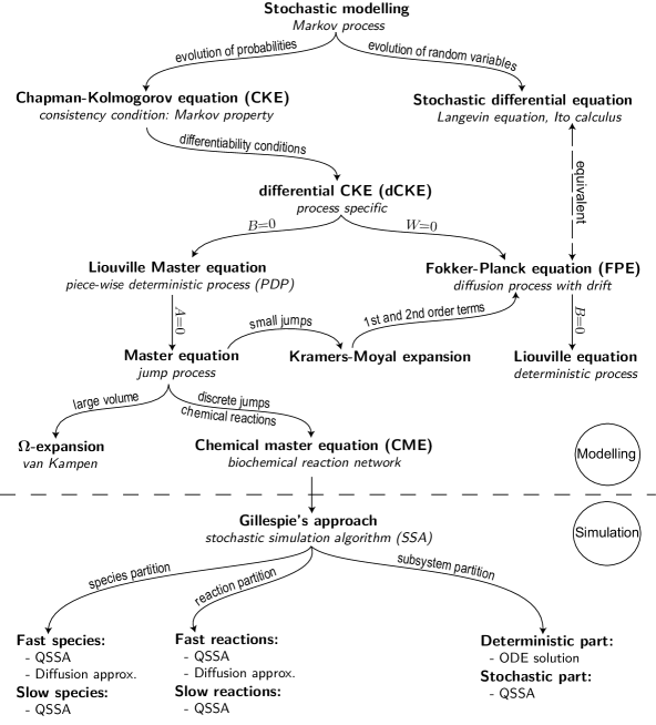
Figure 2: Interrelationships for the stochastic models and their simulation which are covered in this paper. The coefficients $A,B,W$ respectively refer to the drift-vector, diffusion-matrix and the transition-rate in the dCKE. QSSA stands for Quasi-Steady-State Assumption.

This completes our formal analysis and we now return to application of the CME in systems biology.

6 Master equations in systems biology

The chemical master equation (16) is the basis for most stochastic models in systems biology. For complex systems, involving large numbers of chemical species and reactions, the computational cost may be considerable. For this reason modifications to the algorithm and strategies to simplify the model prior to a computer simulation have been suggested. The efforts to reduce the computational complexity of stochastic approaches can be grouped into approximate stochastic methods and hybrid methods. Approximate stochastic methods try to speed up the simulation by compromising exactness of the master equation whereas the hybrid methods treat parts of the system deterministically and other parts stochastically. What follows is a brief discussion of the systems biology literature, using the CME and SSA, including strategies that have been developed to reduce the computational complexity.

6.1 Approximate stochastic methods

In [gillespie:01] Gillespie presents an approximate and thereby faster simulation method known as the $\tau$-leap method. Instead of simulating individual reactions, the number of reactions of each type in a sequence of short time intervals is simulated. Optimal ways to select the leap-length of the intervals have been investigated in [gillespie:03, cao:06]. In [rao:03] Rao et al. propose a reduction of a chemical system by partitioning molecular species into slow (primary) and fast (intermediate) molecular species. Assuming that the intermediate species (conditional on the primary species) are Markovian, they apply the quasi-steady-state assumption (QSSA) which essentially assumes that the conditional probability distribution of the intermediate species is time-invariant (i.e., it has reached a steady-state); thereby eliminating these species from the chemical master equation. A modified version of Gillespie algorithm is subsequently proposed to simulate the resulting reduced system for slow species. In [haseltine:02, haseltine:05] Haseltine and coworker also use the partitioning method for reduction, but partition chemical reactions into fast and slow reactions. The fast reactions are approximated by using Langevin or deterministic equations. The coefficients of the reduced chemical master equation are influenced by the fast reactions. The authors propose simulation algorithms for the slow reactions, subject to constraints imposed by fast reactions. The idea of partitioning to speed up slow-scale simulation has also been used in [cao:05, cao:05a, cao:05b, goutsias:05]. salis:05 present a probabilistic steady-state approximation that separates the time scales of an arbitrary reaction network, detects the convergence of a marginal distribution to a quasi-steady-state, directly samples the underlying distribution, and uses those samples to predict the state of the system. elf:03a propose that, in case of higher dimensions, the master equation could be approximated by the FPE and then discretised in space and time by a finite difference method. They demonstrate the method for a four-dimensional problem in the regulation of cell processes and compare it to the Monte Carlo method of Gillespie. paulsson:00a use the CME to analyse a negative feedback system composed of two species regulating the synthesis of each other. In [paulsson:04] Paulsson uses a variant of the fluctuation-dissipation theorem to give a generic expression for noise arising from different cellular processes, applying the theorem to a simple generic model representing simple gene expression. Paulsson uses the notion of an $\Omega$-expansion of the master equation, i.e., a Taylor series expansion in powers of $1/\Omega$, where $\Omega$ is a system size parameter [kampen:92]. The first- and second- order terms of the expansion reproduce the macroscopic rate equations and realise the fluctuation-dissipation theorem respectively. An equation that decomposes the intrinsic and extrinsic noise contributions is derived to simplify the analysis. elf:03 give a general method to simplify the master equation in a linear noise approximation (LNA), obtained through an $\Omega$-expansion of the master equation. They derive the LNA for the stationary state of a general system of chemical reactions and use it to estimate sizes, correlations and time scales of stochastic fluctuations. They demonstrate that the LNA allows a rapid characterisation of stochastic properties for intracellular networks over a large parameter space. They also show that the LNA can be made more accurate in cases where fast variables can be eliminated from the system. In [elf:03a] the same authors use the LNA of the master equation to characterise intracellular metabolite fluctuations. In both publications, the results of the LNA are compared to simulation of the master equation.

6.2 Hybrid methods

alfonsi:05 present a simulation approach for hybrid stochastic and deterministic reaction models. The system is adaptively partitioned into deterministic and stochastic parts based on a given criteria at each time step of the simulation. They present two algorithmic schemes. The ‘direct hybrid method’ explicitly calculates which reaction occurs and when it occurs. The ‘first and next reaction method’ generates a putative time for each reaction. The reaction corresponding to the smallest time is chosen to occur; the state according updated and the process repeated. lipniacki:06 derive the first-order partial differential equations for probability distribution function from stochastic differential equations describing approximate kinetics of a single cell. Resulting equations are used to calculate mRNA-protein distribution in the case of single gene regulation and the protein-protein distribution in the case of two-gene regulatory systems. In [lipniacki:06a] the same authors present a hybrid stochastic and deterministic treatment of the NF-$\kappa$B regulatory module to analyse a single cell regulation. They combine ordinary differential equations, used for the description of fast reaction channels of processes involving a large number of molecules, with a stochastic switch to account for the activity of the genes involved. Paszek:07 makes two approximations to the exact stochastic description of a gene regulatory network: the continuous approximation considering only the stochasticity due to the gene activity; and the mixed approximation attributing the additional stochasticity to the mRNA transcription/decay process. The underlying distribution is then described by a system of partial differential equations derived from the dCKE after specific assumptions on the coefficients $A,B$ and $W$. kummer:05 take a different approach by deciding on the fly which approach to use. Studying the stochastic simulation of signal transduction via calcium, the authors observe that the transition from stochastic to deterministic occurs within a range of particle numbers that depends the phase space of the system.

Yet another approach is given in [ochiai:05] where a novel multidimensional stochastic framework is proposed to model multi-gene expression dynamics. Inspired by the dCKE, they propose a new experimental scheme which will measure the instantaneous transition probabilities. Given experimental data, one could obtain the coefficients of the dCKE, which can then be solved to obtain the distribution and the corresponding moments and correlations. dublanche:06 analyse noise in a negatively feedback-regulated transcription factor (TF) and the effects of the feedback loop on a gene repressed by the same TF using a modified Gillespie algorithm (provided by SmartCell). The authors find that within a certain range of repression strength, the negative feedback loop minimises the noise whereas outside this range, noise is increased. It is proposed that this may arise from plasmid fluctuations.

7 Conclusions

The application of stochastic models is usually motivated by uncertainty arising from variability. In the engineering and physical sciences the variability arises mainly from measurements. In systems biology the variability arises mainly from the complexity of intracellular processes. By complexity we mean the fact that in a particular biological network we are forced to eliminate many variables that are influencing the observation we make. While the assumptions of constant temperature, pH level, volume and water balance may not worry most modellers, the large number of unmodelled variables may be of greater concern. Implicit in most stochastic models is the assumption of a well-mixed homogeneous environment in which there are more non-reactive collisions than the reactive ones. More realistic spatial representations are therefore an increasingly important research theme in systems biology. In gene expression a very small number of molecules controls potentially very large molecular populations, suggesting hybrid approaches to combine stochastic and deterministic formalisms. Many cellular processes, for instance the differentiation of stem cells, are multistable systems for which state-of-the-art single-cell measurements are providing increasingly valuable data with nanometre and millisecond resolution. The advance of these technologies allows us to monitor the transcription of individual genes, leading also to a demand for advanced stochastic modelling and simulation.

Motivated by applications of stochastic models in systems biology, we described a probabilistic framework based on Markov processes to represent biochemical reaction networks. We provided a novel derivation of the differential Chapman-Kolmogorov equation for a general Markov process made up of both continuous and jump processes. Then we reviewed the formal relationships between the equations referred to in the systems biology literature, establishing a “family tree” for stochastic models in systems biology, providing explicit derivations of their formal relationship and clarifying assumptions involved in a common framework (See Figure 2). Our derivation starts with the definition of a time-derivative unlike Gardiner who starts with the expectation of an arbitrary function. We place no restrictions on the probability distribution, whereas Gardiner assumes it to be confined to a region that has a surface, and the probability being zero on the surface. The master equation gives the jump part of the Markov process while the FPE gives the continuous part. The derivation of FPE in breuer:02 and kampen:92 involves approximation of the master equation by investigating the limit of a jump process.