Quasispecies Theory for Multiple-Peak Fitness Landscapes

Abstract

We use a path integral representation to solve the Eigen and Crow-Kimura molecular evolution models for the case of multiple fitness peaks with arbitrary fitness and degradation functions. In the general case, we find that the solution to these molecular evolution models can be written as the optimum of a fitness function, with constraints enforced by Lagrange multipliers and with a term accounting for the entropy of the spreading population in sequence space. The results for the Eigen model are applied to consider virus or cancer proliferation under the control of drugs or the immune system.

I Introduction

It is widely accepted that biological evolution proceeds on a rugged fitness landscape Wright (1931); Kauffmann and Levin (1987). In the last decade, several exact results Baake et al. (1997); Saakian and Hu (2004a, b) have been derived for the molecular evolution models of Eigen Eigen (1971); Eigen et al. (1989) and Crow-Kimura Crow and Kimura (1970) and their generalizations Messer et al. (2005).

In this paper, we consider a multiple-peak replication rate landscape as a means to model a rugged fitness landscape. To date, there are few rigorous results for multiple-peak fitness landscapes. Such results begin to make the connection with the biologically-relevant case of a rugged fitness landscape. We here derive error thresholds by means of a path integral representation for both the Eigen and Crow-Kimura mutation-selection schemes with an arbitrary number of replication rate peaks.

We first generalize the Crow-Kimura model to the multiple-peak case. The solution of the single-peak version of this model, where the replication rate is a function of the Hamming distance from one configuration, was provided by a path integral representation in Saakian and Hu (2004a, b); Saakian et al. (2004). We here provide the solution to this model for $K$ peaks, where the replication rate is a function of the Hamming distances from $K$ configurations, again by means of a path integral. We find that the mean distances from the peaks maximize the replication rate, with constraints provided by Lagrange multipliers, and with an additional term that represents the entropy of the population in sequence space. Explicit solutions to this maximization task are given for the two-peak case.

We then generalize and solve the continuous-time Eigen model for $K$ peaks, where the replication and degradation rates are functions of the Hamming distances from $K$ configurations, A solution of the discrete-time, single-peak Eigen model, which in a sense interpolates between the Crow-Kimura and continuous-time Eigen model Jain and Krug (2005), was provided in Peliti (2002). We here solve the continuous-time Eigen model for $K$ peaks, again by means of a path integral representation. The mean distances from the peaks maximize an excess replication rate with an effective mutation rate, with constraints provided by Lagrange multipliers, and with an additional term that represents the entropy of the population in sequence space under the effective mutation rate.

The Eigen model was first developed to study viral evolution Eigen (1971), and we use our solution of the two-peak Eigen model to consider viral propagation in the presence of either immune system suppression or an anti-viral drug. The preferred viral genome exists at one point in genome space. Conversely, the drug or immune system suppresses the virus most strongly at some other point in genome space. These two points in genome space are the two peaks of the model. The viral growth rate and the suppression rate both decrease with the Hamming distance away from these two unique points.

The rest of the paper is organized as follows. In Section 2 we describe the generalization of the Crow-Kimura, or parallel, model to multiple peaks. We provide a solution of this model for an arbitrary replication rate function that depends on distances from $K$ peaks. In Section 3, we describe the Eigen model. We provide a solution for arbitrary replication and degradation rate functions that depend on distances from $K$ peaks. In Section 4, we use the Eigen model theory to address the interaction of the immune system with a drug. We consider both adaptable drugs and the original antigenic sin phenomenon Deem and Lee (2003). We also consider tumor suppression by the immune system. We discuss these results and conclude in section 5. We provide a derivation of the path integral representation of the continuous-time Eigen model in the Appendix.

II Crow-Kimura model with multiple peaks

Here we first briefly introduce the Crow-Kimura model Crow and Kimura (1970) and its quantum spin version Baake et al. (1997) so that it is easier to understand its generalizations to be studied in the present paper. In the Crow-Kimura model, any genotype configuration $i$ is specified a sequence of $N$ two-valued spins $s_{n}=\pm 1$, $1\leq n\leq N$. We denote such configuration $i$ by $S_{i}\equiv({s_{1}^{i},\dots,s_{N}^{i}})$. That is, as in Eigen et al. (1989), we consider $s_{n}=+1$ to represent the purines (A, G) and $s_{n}=-1$ to represent the pyrimidines (C, T). The difference between two configurations $S_{i}$ and $S_{j}\equiv({s_{1}^{j},\dots,s_{N}^{j}})$ is described by the Hamming distance $d_{ij}=(N-\sum_{n}s_{n}^{i}s_{n}^{j})/2$, which is the number of different spins between $S_{i}$ and $S_{j}$. The relative frequency $p_{i}$ of configurations with a given sequence $1\leq i\leq 2^{N}$ satisfies

$$\frac{{dp}_{i}}{dt}={p_{i}}(r_{i}-{\sum}_{j=1}^{2^{N}}r_{j}p_{j})+{\sum}_{j=1}^{2^{N}}\mu_{ij}p_{j}\ .$$ (1)

Here $r_{i}$ is the the replication rate or the number of offspring per unit period of time, the fitness, and $\mu_{ij}$ is the mutation rate to move from sequence $S_{i}$ to sequence $S_{j}$ per unit period of time. In the Crow-Kimura model, only single base mutations are allowed: $\mu_{ij}=\gamma\Delta(d_{ij}-1)-N\gamma\Delta(d_{ij})$. Here $\Delta(n)$ is the Kronecker delta.

The fitness of an organism with a given genotype is specified in the Crow-Kimura model by the choice of the replication rate function $r_{i}$, which is a function of the genotype: $r_{i}=f(S_{i})$. It has been observed Baake et al. (1997) that the system (1), with $r_{i}\equiv f(s_{1}^{i},\dots,s_{N}^{i})$ evolves according to a Schrödinger equation in imaginary time with the Hamiltonian:

$$-H=\gamma\sum_{n=1}^{N}(\sigma^{x}_{n}-1)+f(\sigma_{1}^{z},\ldots,\sigma_{N}^{z})\ .$$ (2)

Here $\sigma^{x}$ and $\sigma^{z}$ are the Pauli matrices. The mean replication rate, or fitness, of the equilibrium population of genotypes is calculated as $\lim_{t\to\infty}\sum_{i}p_{i}(t)r_{i}=\lim_{\beta\to\infty}\frac{1}{\beta}\ln Z\equiv\lim_{\beta\to\infty}\frac{1}{\beta}\ln Tr\exp(-\beta H)$ Eigen et al. (1989). In this way it is possible to find the phase structure and error threshold of the equilibrium population. In the generalized setting, the Crow-Kimura model is often called the parallel model.

II.1 The parallel model with two peaks

We consider two peaks to be located at two configurations $v^{1}_{n},v^{2}_{n},1\leq n\leq N$, where $v^{1}_{n}=\pm 1,v^{2}_{n}=\pm 1$, and the two configurations have $l$ common spins: $\sum_{n=1}^{N}v^{1}_{n}v^{2}_{n}=2l-N$. The value of $l$ determines how close the two peaks are in genotype space. Now the replication rate of configuration $S$ is a function of the Hamming distances to each peak:

$$r_{i}=f(2L_{1}/N-1,2L_{2}/N-1)\ ,$$ (3)

where $\sum_{n=1}^{N}v^{1}_{n}s_{n}=2L_{1}-N$ and $\sum_{n=1}^{N}v^{2}_{n}s_{n}=2L_{2}-N$.

Due to the symmetry of the Hamiltonian, the equilibrium frequencies are a function only of the distances from the two peaks: $p_{i}\equiv p(L_{1},L_{2})$. We define the factors $x_{\alpha_{1},\alpha_{2}}$ that describe the fraction of spins a configuration $S$ has in common with the spins of configurations $v^{1},v^{2}$. In particular, we define the fraction of spins that are equal to $\alpha_{k}$ times the value in peak configuration $v^{k}$. For $K$ peaks, the general definition is $x_{\alpha_{1}\ldots\alpha_{K}}=(1/N)\sum_{n=1,N}\delta[s_{n},\alpha_{1}v_{n}^{1}]\dots\delta[s_{n},\alpha_{K}v_{n}^{K}]$. For the two peak case, these factors are related to the distances from the configuration to each peak and to the distance between the peaks:

$$x_{+-}(L_{1},L_{2}) = (L_{1}-L_{2}+N-l)/(2N)$$

$$x_{++}(L_{1},L_{2}) = (L_{1}+L_{2}-N+l)/(2N)$$

$$x_{--}(L_{1},L_{2}) = (-L_{1}-L_{2}+N+l)/(2N)$$

$$x_{-+}(L_{1},L_{2}) = (-L_{1}+L_{2}+N-l)/(2N)\ .$$ (4)

With these factors $x$, we find the following equation for the total probability at a given value of $L_{1}$ and $L_{2}$, $P(L_{1},L_{2})$:

$$\frac{dP(L_{1},L_{2})}{dt}=f(\frac{2L_{1}}{N}-1,\frac{2L_{2}}{N}-1)P(L_{1},L_{2})$$

$$-\gamma NP(L_{1},L_{2})$$

$$+\gamma\sum_{\alpha_{1}=\pm 1,\alpha_{2}=\pm 1}Nx_{\alpha_{1},\alpha_{2}}(L_{1}+\alpha_{1},L_{2}+\alpha_{2})$$

$$\times P(L_{1}+\alpha_{1},L_{2}+\alpha_{2})$$

$$-P(L_{1},L_{2})\sum_{L_{1}^{\prime},L_{2}^{\prime}=0}^{N}f(\frac{2L_{1}^{\prime}}{N}-1,\frac{2L_{2}^{\prime}}{N}-1)P(L^{\prime}_{1},L^{\prime}_{2})\ .$$

Only the values of $L_{1}$ and $L_{2}$ satisfying the conditions $0\leq L_{i}\leq N$, $|L_{1}+L_{2}-N|\leq l$, $|L_{1}-L_{2}|\leq N-l$ are associated with non-zero probabilities. Equation (II.1) can be solved numerically to find the error threshold and average distance of the population to the two peaks. In the next section we solve this equation, and its generalization to $K$ peaks, analytically.

II.2 Exact solution of the $K$ peak case by a path integral representation

We consider the case of $K$ peaks. We consider the replication rate to depend only on the distances from each peak

$$r_{i}=f(\frac{2L_{1}}{N}-1,\dots,\frac{2L_{K}}{N}-1)\equiv Nf_{0}(u_{1},\ldots,u_{K})\ ,$$ (6)

where $Nu_{k}=\sum_{n=1}^{N}v^{k}_{n}s_{n}=2L_{k}-N,1\leq k\leq K$. The observable value $\langle u_{k}\rangle$ is called the surface magnetization Tarazona (1992), or surplus Baake et al. (1997), for peak $k$.

Characterization of the fitness function that depends on $K$ peaks through the $K$ values of $u_{k}$ requires more than the $K(K-1)/2$ Hamming distances between the peaks. It proves convenient to define the $2^{K}$ parameters $y_{\alpha_{1}\ldots\alpha_{K}}\equiv y_{i},i\leq i\leq 2^{K}$. These are defined by $y_{i}=(1/N)\sum_{n=1}^{N}\prod_{k=1}^{K}\delta(\alpha_{ik},v_{n}^{k})$. Here $\alpha_{i}$ is the set of indices $\alpha_{1}\ldots\alpha_{K}$, and $\alpha_{ik}=\alpha_{k}$ in a $i$-th set of indices $\alpha_{1}\ldots\alpha_{K}$. The introduction of the $2^{K}$ parameters $y_{i}$ is one principle point of this article.

The Trotter-Suzuki method has been applied in Saakian and Hu (2004b); Saakian et al. (2004) to convert the quantum partition function for a single peak model into a classical functional integral. While calculating $Z\equiv\exp[-\beta H]$, intermediate spin configurations are introduced. We find $Z$ is a functional integral, with the integrand involving a partition function of a spin system in 2-$d$ lattice. In the spin system, there is a nearest-neighbor interaction in horizontal direction and a mean-field like interaction in the vertical direction. This spin system partition function was evaluated in Saakian and Hu (2004b); Saakian et al. (2004) under the assumption that the field values are constant. A path integral representation of the discrete time Eigen model, which is quite similar to the parallel model, was introduced by Peliti Peliti (2002).

We here generalize this procedure to $K$ peaks and calculate the time-dependent path integral and Ising partition function. Since the replication rate is a function of $K$ distances, the functional integral is over $K$ fields that represent the $K$ magnetizations. The path integral form of the partition function is

$$Z = \int{\cal D}M_{k}{\cal D}H_{k}\exp\bigg{\{}N\int_{0}^{\beta}d\beta^{\prime}\bigg{[}f_{0}[M_{1}(\beta^{\prime}),\ldots,M_{K}(\beta^{\prime})]$$ (7)

$$-\sum_{k=1}^{K}H_{k}(\beta^{\prime})M_{k}(\beta^{\prime})-\gamma\bigg{]}+N\sum_{i=1}^{2^{K}}y_{i}\ln Q_{1}\bigg{\}},$$

where

$$Q_{1}=Tr\hat{T}e^{\int_{0}^{\beta}d\beta^{\prime}\left[\sigma^{x}\gamma+\sigma^{z}\sum_{k=1}^{K}\alpha_{ik}H_{k}(\beta^{\prime})\right]}\ .$$ (8)

Here $\beta=t$, is the large time to which Eq. (1) is solved, and the operator $\hat{T}$ denotes time ordering Saakian et al. (2004), discussed in the Appendix in the context of the Eigen model. Using that $N$ is large, we take the saddle point. Considering $\delta\ln Z/\delta M_{k}(\beta^{\prime})=0$ and $\delta\ln Z/\delta H_{k}(\beta^{\prime})=0$, we find $M_{k}(\beta^{\prime})$ and $H_{k}(\beta^{\prime})$ independent of $\beta^{\prime}$ is a solution. At long time, therefore, the mean replication rate, or fitness, per site becomes

$$\frac{\ln Z}{\beta N} = \max_{M_{k},H_{k}}\bigg{\{}f_{0}(M_{1},\ldots,M_{K})-\sum_{k=1}^{K}H_{k}M_{k}-\gamma$$ (9)

$$+\sum_{i=1}^{2^{K}}y_{i}\left[\gamma^{2}+(\sum_{k=1}^{K}\alpha_{ik}H_{k})^{2}\right]^{1/2}\bigg{\}}\ .$$

We take the saddle point in $H_{k}$ to find

$$M_{k}=\sum_{i}y_{i}\alpha_{ik}\frac{\sum_{k^{\prime}=1}^{K}\alpha_{ik^{\prime}}H_{k^{\prime}}}{\sqrt{\gamma^{2}+(\sum_{k^{\prime}=1}^{K}\alpha_{ik^{\prime}}H_{k^{\prime}})^{2}}}\ .$$ (10)

We note that the observable, surface, magnetization given by $\langle u_{k}\rangle$ is not directly accessible in the saddle point limit, but is calculable from the mean replication rate Baake et al. (1997). In the one peak case one defines the observable surface magnetization for a monotonic fitness function as follows Baake et al. (1998): one solves the equation $f_{0}(\langle u\rangle)=(\ln Z)/(\beta N)$. For multiple peaks, we use this same trick, considering a symmetric fitness function and assuming $\langle u_{1}\rangle=\langle u_{2}\rangle\dots=\langle u_{K}\rangle$.

II.3 Explicit results for the two peak case

For clarity, we write the expression for the case of two peaks. In this case, $y_{++}+y_{--}=(1+m)/2$ and $y_{+-}+y_{-+}=(1-m)/2$, where $m=(2l-N)/N$. We solve Eq. (10) for the fields $H_{k}$ and put the result into Eq. (9). We find that for a pure phase, the bulk magnetizations maximize the function

$$\frac{\ln Z}{N\beta} = f_{0}(M_{1},M_{2})$$ (11)

$$+\frac{\gamma}{2}\sqrt{(1+m)^{2}-(M_{1}+M_{2})^{2}}$$

$$+\frac{\gamma}{2}\sqrt{(1-m)^{2}-(M_{1}-M_{2})^{2}}-\gamma\ ,$$

with the constraints

$$-1\leq M_{1}\leq 1;\quad-1\leq M_{2}\leq 1$$

$$-(1+m)\leq M_{1}+M_{2}\leq 1+m$$

$$\quad-(1-m)\leq M_{1}-M_{2}\leq 1-m\ .$$ (12)

In the case of a quadratic replication rate, $f_{0}=k_{1}M_{1}^{2}+k_{2}M_{2}^{2}+k_{3}M_{1}M_{2}$, Eq. (11) becomes

$$\frac{\ln Z}{N\beta} = k_{1}M_{1}^{2}+k_{2}M_{2}^{2}+k_{3}M_{1}M_{2}$$ (13)

$$+\frac{\gamma}{2}\sqrt{(1+m)^{2}-(M_{1}+M_{2})^{2}}$$

$$+\frac{\gamma}{2}\sqrt{(1-m)^{2}-(M_{1}-M_{2})^{2}}-\gamma\ ,$$

with the constraints of Eq. (II.3).

As an example, we consider the replication rate function $f_{0}=k(M_{1}^{2}+M_{2}^{2}+M_{1}M_{2})/2$. When $m\geq 0$, and the two peaks are within a Hamming distance of $N/2$ of each other, there is a solution with $M_{1}=M_{2}=M$ for which

$$\frac{3kM^{2}}{2\gamma}+\left[\left(\frac{1+m}{2}\right)^{2}-M^{2}\right]^{1/2}-\frac{1+m}{2}$$

$$=\frac{k}{2\gamma}\left(\langle u_{1}\rangle^{2}+\langle u_{2}\rangle^{2}+\langle u_{1}\rangle\langle u_{2}\rangle\right)\ ,$$ (14)

where the observable, surface, magnetization is given by $\langle u_{i}\rangle=\langle 2L_{i}/N-1\rangle$. We find

$$M_{1}=M_{2}=M=\sqrt{(1+m)^{2}/4-\gamma^{2}/(9k^{2})}\ .$$ (15)

We have for the mean replication rate, or fitness, per site

$$\frac{\ln Z}{\beta N}=\frac{3k}{2}\left(\frac{1+m}{2}-\frac{\gamma}{3k}\right)^{2}\ ,$$ (16)

so that Baake et al. (1997)

$$\langle u\rangle=\frac{1+m}{2}-\frac{\gamma}{3k}\ .$$ (17)

When $m<0$, and the two peaks are greater than a Hamming distance of $N/2$ of each other, there is a solution with $M_{1}=-M_{2}=M$ for which

$$\frac{kM^{2}}{2\gamma}+\left[(\frac{1-m}{2})^{2}-M^{2}\right]^{1/2}-\frac{1-m}{2}$$

$$=\frac{k}{2\gamma}\left(\langle u_{1}\rangle^{2}+\langle u_{2}\rangle^{2}+\langle u_{1}\rangle\langle u_{2}\rangle\right)\ .$$ (18)

One solution is

$$M_{1}=-M_{2}=\sqrt{(1-m)^{2}/4-\gamma^{2}/k^{2}}\ ,$$ (19)

which gives for a mean replication rate, or fitness, per site

$$\frac{\ln Z}{\beta N}=\frac{k}{2}\left(\frac{1-m}{2}-\frac{\gamma}{k}\right)^{2}\ ,$$ (20)

so that Baake et al. (1997)

$$\langle u_{1}\rangle=-\langle u_{2}\rangle=\frac{1-m}{2}-\frac{\gamma}{k}\ .$$ (21)

Numerical solution is in agreement with our analytical formulas, as shown in Table 1.

m	k	$\langle u_{1}\rangle$	$\langle u_{2}\rangle$	$\langle u_{1}\rangle_{\rm analytic}$	$\langle u_{2}\rangle_{\rm analytic}$
0.93	3.0	0.85	0.85	0.853	0.853
0.93	2.0	0.80	0.80	0.798	0.798
0.7	3.0	0.74	0.74	0.738	0.738
0.7	2.0	0.68	0.68	0.683	0.683
-0.7	3.0	0.52	-0.52	0.517	-0.517
-0.7	2.0	0.35	-0.35	0.35	-0.35
-0.93	3.0	0.63	-0.63	0.631	-0.631
-0.93	2.0	0.46	-0.46	0.465	-0.465

Table 1: Comparison between the analytical formulas Eqs. (17, 21) for the two peak landscape in the parallel model and results from a direct numerical solution of the system of differential equations, Eq. (II.1), for sequences of length $N=1000$, with $p(L_{1},L_{2},t=0)=\delta(L_{1},N)\delta(L_{2},l)$.

III Eigen model with multiple peaks

III.1 Exact solution by a path integral representation

In the case of the Eigen model, the system is defined by means of replication rate functions, $r_{j}$, as well as degradation rates, $D_{j}$:

$$\frac{dp_{i}}{dt}=\sum_{j=1}^{2^{N}}\left[Q_{ij}r_{j}-\delta_{ij}D_{j}\right]p_{j}-p_{i}\left[\sum_{j=1}^{2^{N}}(r_{j}-D_{j})p_{j}\right]\ .$$ (22)

Here the frequencies of a given genome, $p_{i}$, satisfy $\sum_{i=1}^{2^{N}}p_{i}=1$. The transition rates are given by $Q_{ij}=q^{N-d(i,j)}(1-q)^{d(i,j)}$, with the distance between two genomes $S_{i}$ and $S_{j}$ given by $d(i,j)=(N-\sum_{n=1}^{N}s_{n}^{i}s_{n}^{j})/2$. The parameter $\gamma=N(1-q)$ describes the efficiency of mutations. We take $\gamma=O(1)$. As in Eq. (6), we take the replication and degradation rate to depend only on the spin state, in particular on the distances from each peak: $r_{i}=f(S_{i})$ and $D_{i}=D(S_{i})$ where

$$f(S)=Nf_{0}(u_{1},\ldots,u_{k}),~{}D(S)=Nd_{0}(u_{1},\ldots,u_{k})\ .$$ (23)

We find the path integral representation of the partition function for the Eigen model for the $K$ peak case in the limit of long time as

$$Z = \int{\cal D}M_{k}{\cal D}H_{k}{\cal D}m_{0}{\cal D}h_{0}\exp\bigg{\{}N\int_{0}^{\beta}d\beta^{\prime}\bigg{[}$$ (24)

$$f_{0}(M_{1},\ldots,M_{K})e^{-\gamma(1-m_{0})}-h_{0}m_{0}$$

$$-\sum_{k=1}^{K}H_{k}M_{k}-d_{0}(M_{1},\ldots,M_{K})\bigg{]}$$

$$+N\sum_{i=1}^{2^{K}}y_{i}\ln Q_{1}\bigg{\}}\ ,$$

where

$$Q_{1}=Tr\hat{T}e^{\int_{0}^{\beta}d\beta^{\prime}\left[\sigma^{x}h_{0}(\beta^{\prime})+\sigma^{z}\sum_{k=1}^{K}\alpha_{ik}H_{k}(\beta^{\prime})\right]}\ .$$ (25)

The $M_{k}$ are the values of the magnetization, and $\gamma m_{0}$ is an effective mutation rate. This form is derived in the Appendix. Using that $N$ is large, we take the saddle point. As before, we find the mean excess replication rate per site, $f_{m}=\lim_{t\to\infty}\sum_{i}p_{i}(t)(r_{i}-D_{i})/N$, from the maximum of the expression for $Z={\rm Tr}\exp(-\beta H)$. We find $Z\sim\exp(\beta Nf_{m})$, where

$$f_{m} = f_{0}(M_{1},\ldots,M_{K})e^{-\gamma(1-\sum_{i=1}^{2^{K}}y_{i}\sqrt{1-m_{i}^{2}})}$$ (26)

$$-d_{0}(M_{1},\ldots,M_{K})\ ,$$

and where $m_{0},M_{k}$ are defined through the fields $H_{k}$:

$$M_{k} = \sum_{i}y_{i}\alpha_{ik}\frac{\sum_{k^{\prime}=1}^{K}\alpha_{ik^{\prime}}H_{k^{\prime}}}{\sqrt{h_{0}^{2}+(\sum_{k^{\prime}=1}^{K}\alpha_{ik^{\prime}}H_{k^{\prime}})^{2}}}$$

$$m_{0} = \sum_{i}y_{i}\frac{h_{0}}{\sqrt{h_{0}^{2}+(\sum_{k=1}^{K}\alpha_{ik}H_{k})^{2}}}\ .$$ (27)

We define

$$m_{i}=\frac{\sum_{k=1}^{K}\alpha_{ik}H_{k}}{\sqrt{h_{0}^{2}+(\sum_{k=1}^{K}\alpha_{ik}H_{k})^{2}}}\ .$$ (28)

We thus find $m_{0}=\sum_{i=1}^{2^{K}}y_{i}\sqrt{1-m_{i}^{2}}$, giving Eq. (26).

III.2 Eigen model with quadratic replication rate without degradation

We apply our results to model qualitatively the interaction of a virus with a drug. In some situations, one can describe the action of a drug against the virus simply as a one peak Eigen model: that is, replication rate is a function of the Hamming distance from one peak. The virus may increase its mutation rate, and at some mutation rate there is an error catastrophe Eigen (2002). Let us define the critical $\gamma$ for the replication rate function

$$f_{0}(M)=kM^{2}/2+1\ .$$ (29)

According to our analytical solution, Eq. (26), we consider the maximum of the mean excess replication rate per site expression

$$f_{0}(M)\exp[-\gamma(1-\sqrt{1-M^{2}})]\ .$$ (30)

The error catastrophe occurs and leads to a phase with $M=0$ when $k<\gamma$. The error threshold for this quadratic case is the same as in the case of the Crow-Kimura model Eq. (1). Numerical solution is in agreement with our analytical formulas, as shown in Table 2.

$k/\gamma$	M	$\langle u\rangle$	$\langle u\rangle_{\rm analytic}$
1.2	0.24	0.065	0.068
1.4	0.31	0.112	0.113
1.6	0.35	0.146	0.147
1.8	0.38	0.172	0.172
2.0	0.41	0.192	0.193

Table 2: Comparison between the analytical formulas Eqs. (30) for the quadratic landscape (29) in the Eigen model and results from a direct numerical solution of the system of differential equations Eigen et al. (1989), for sequences of length $N=4000$, with $p(u,t=0)=\delta(u,1)$. We set $\gamma=5$.

III.3 Simple formulas for two peak case

In the two peak, $K=2$, case we can define the $m_{i}$ from Eq. (28) from the system

$$M_{1} = \frac{1+m}{2}(m_{1}+m_{2})+\frac{1-m}{2}(m_{1}-m_{2})$$

$$M_{2} = \frac{1+m}{2}(m_{1}+m_{2})-\frac{1-m}{2}(m_{1}-m_{2})\ ,$$ (31)

where we have defined $m_{1},m_{2}$ in terms of the $m_{i}$ from Eq. (28) by $m_{++}=-m_{--}=m_{1}+m_{2}$ and $m_{+-}=-m_{-+}=m_{1}-m_{2}$  , We have for the mean excess replication rate per site

$$f_{m} = f_{0}(M_{1},M_{2})\exp\bigg{[}-\gamma\bigg{(}1$$ (32)

$$-\frac{1+m}{2}\sqrt{1-(M_{1}+M_{2})^{2}/(1+m)^{2}}$$

$$-\frac{1-m}{2}\sqrt{1-(M_{1}-M_{2})^{2}/(1-m)^{2}}\bigg{)}\bigg{]}$$

$$-d_{0}(M_{1},M_{2})\ .$$

IV Biological applications

The Eigen model is commonly used to consider virus or cancer evolution. We here consider an evolving virus or cancer and its control by a drug or the immune system, using the $K=2$, two-peak version of the Eigen model. To model this situation, we consider there to be an optimal genome for virus replication, and we consider the replication rate function $f_{0}(M_{1},M_{2})$ to depend only on the Hamming distance of the virus or cancer from this preferred genome, $N(1-M_{1})/2$. Conversely, there is another point in genome space that the drug or immune suppresses most strongly, and we consider the degradation rate function $d_{0}(M_{1},M_{2})$ to depend only on the Hamming distance from this point, $N(1-M_{2})/2$. While each of the functions $f_{0}$ and $d_{0}$ depend only on one of the two distances, this is multiple-peak problem, because both distances are needed to describe the evolution of the system.

IV.1 Interaction of virus with a drug

We first consider a virus interacting with a drug. We model this situation by the Eigen model with one peak in the replication rate function and one peak in the degradation rate function. The virus replicates most quickly at one point in genome space, with the rate at all other points given by a function that depends on the Hamming distance from this one point. That is, in Eq. (32) we have

$$f_{0}(M_{1},M_{2})=\left\{\begin{array}[]{lll}&A,&\,\,M_{1}=1\\ &&\\ &1,&\,\,M_{1}<1\end{array}\right.\ .$$ (33)

At another point in genome space, a drug suppresses the virus most strongly. We consider the case of exponential degradation, a generic and prototypical example of recognition Deem and Lee (2003):

$$d_{0}(M_{1},M_{2})=e^{-b(1-M_{2})}\ .$$ (34)

Applying the multiple-peak formalism, we find two phases. There is a selected, ferromagnetic (FM) phase with $M_{1}=1$, $M_{2}=m$ and mean excess replication rate per site

$$f_{m}=Ae^{-\gamma}-\exp(-b(1-m))\ .$$ (35)

There is also a non-selective $NS$ phase, with $M_{1}<1$. The values of $M_{1}$ and $M_{2}$ in the NS phase are those which maximize Eq. 32 given the constraints of Eq. (II.3). The error threshold corresponds to the situation when the mean excess replication rate of the FM and NS phases are equal. The phase diagram as a function of the optimal replication rate of the virus and the distance between the points of optimal virus growth and optimal virus suppression is shown in Fig. 1. The optimal replication rate is $A$, and the distance between the points of optimal virus growth and optimal virus suppression is $N-l$, where the parameter $m$ is defined as $m=(2l-N)/N$. As the point in genome space at which the drug is most effective moves toward the point in genome space at which the virus grows most rapidly, the virus is more readily eradicated. Alternatively, one can say that as the point in genome space at which the drug is most effective moves toward the point in genome space at which the virus grows most rapidly, a higher replication rate of the virus is required for its survival.

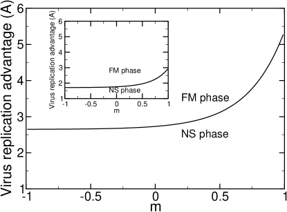
Figure 1: A phase diagram for the interaction of virus and drug, according to the narrow replication advantage model, Eqs. (34) and (33). We set $b=3.5$ in the exponential degradation function Eq. (34), and $\gamma=1$. As the point in genome space at which the drug is most effective moves toward the point in genome space at which the virus grows most rapidly, $m\to 1$, a higher replication rate of the virus is required for the virus to survive. In the NS phase, the drug eliminates the virus. In inset is shown the phase diagram for the interaction of an adaptable virus and a drug, according to the flat peak replication advantage model, Eqs. (34) and (39). We use $M_{0}=0.9$ to represent a broad peak for the virus replication rate.

IV.2 Interaction of an adaptable virus with a drug

We now consider a virus that replicates with rate $A$ when the genome is within a given Hamming distance from the optimal genome and with rate $1$ otherwise. That is, in Eq. (32) we have

$$f_{0}(M_{1},M_{2})=\left\{\begin{array}[]{lll}&A,&\,\,M_{0}\leq M_{1}\leq 1\\ &&\\ &1,&\,\,-1\leq M_{1}<M_{0}\end{array}\right.\ ,$$ (39)

where $M_{0}>0$ and close to one. We suppression of the virus by the drug as expressed in Eq. (34).

There is again a ferromagnetic (FM) phase with a successful selection. In the FM phase, one has $M_{0}\leq M_{1}\leq 1$. The evolved values of $M_{1}$ and $M_{2}$ maximize

$$f_{m} = A\exp\bigg{[}-\gamma\bigg{(}1$$ (40)

$$-\frac{1+m}{2}\sqrt{1-(M_{1}+M_{2})^{2}/(1+m)^{2}}$$

$$-\frac{1-m}{2}\sqrt{1-(M_{1}-M_{2})^{2}/(1-m)^{2}}\bigg{)}\bigg{]}$$

$$-d_{0}(M_{1},M_{2})\ .$$

There is also a NS phase where the virus has been driven off its advantaged peak, $M_{1}<M_{0}$. In this case, one seeks a maximum of Eq. (32) with $f_{0}=1$ via $M_{1}$ and $M_{2}$ in the range $-1\leq M_{1}\leq M_{0}$, $-1\leq M_{2}\leq 1$, subject to the constraints of Eq. (II.3).

A phase diagram for this case is shown in the inset to Fig. 1. The broader range of the virus fitness landscape allows the virus to survive under a greater drug pressure in model Eq. (39) versus Eq. (33). That is, as the point in genome space at which the drug is most effective moves toward the point in genome space at which the virus grows most rapidly, the adaptable virus is still able to persist due to the greater range of genotype space available in the FM phase. For such an adaptable virus, a more specific, multi-drug cocktail might be required for eradication. A multi-drug cocktail provides more suppression in a broader range of genome space, so that the adaptable drug may be eradicated under a broader range of conditions.

IV.3 Original antigenic sin

The immune system acts much like a drug, as a natural protection against death by infection. Prior exposure such as vaccination typically increases the immune control of a virus. In some cases, the immune control of a virus is non-monotonic in the distance between the vaccine and the virus Deem and Lee (2003). This phenomenon is termed original antigenic sin. To model original antigenic sin, we consider a non-monotonic degradation function, centered around the second peak, which represents the non-monotonic behavior of the binding constant, as in our previous model Deem and Lee (2003). We fit the binding constant data Deem and Lee (2003) to a sixth order polynomial in $p$, where $p=(1-M_{2})/2$ is the relative distance between the recognition of the antibody and the virus. The degradation function is shown in inset in Fig. 2. We consider a single peak virus replication rate, Eq. (33).

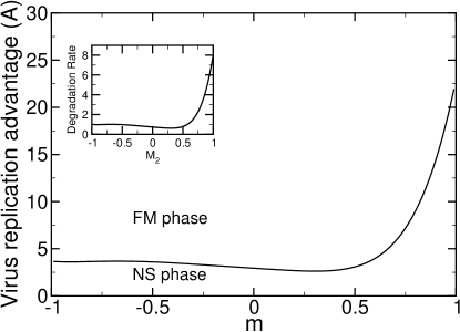
Figure 2: A phase diagram corresponding to the original antigenic sin model is shown. The degradation function (shown in inset) is chosen to closely reproduce the binding constant behavior in Deem and Lee (2003), with a limiting degradation rate of $d_{0}(M_{1},M_{2}=-1)=1$. We use $\gamma=1$. The virus replication advantage required to escape immune system control is a non-monotonic function of the Hamming distance, $N(m-1)/2$, between the point in genome space at which the immune system is most effective and the point in genome space at which the virus grows most rapidly.

There is an interesting phase structure as a function of $m$. From Eq. (32), we have a FM phase with $M_{1}=1$, $M_{2}=m$. We also have a non-selective NS phase, with $M_{1}<1$, where $M_{1},M_{2}$ are determined by maximization of Eq.  (32) with $f_{0}=1$ under the constraints of Eq.  (II.3). The phase diagram for typical parameters Deem and Lee (2003), is shown in Fig. 2. A continuous phase boundary is observed between the FM and NS phases. The virus replication rate required to escape eradication by the adaptive immune system depends on how similar the virus and the vaccine are. When the vaccine is similar to the virus, $m$ near 1, a large virus replication rate is required to escape eradication. This result indicates the typical usefulness of vaccines in protection against and eradication of viruses. When the vaccine is not similar to the virus, $m<0$, the vaccine is not effective, and only a typical virus replication rate is required.

When the vaccine is somewhat similar to, but not identical to, the virus, the replication rate required for virus survival is non-monotonic. This result is due to the non-monotonic degradation rate around the vaccine degradation peak. The minimum in the required virus replication rate, $m\approx 0.30$, corresponds to the minimum in the degradation rate, $M_{2}\approx 0.30$. The competition between the immune system, vaccine, and virus results in a non-trivial phase transition for the eradication of the virus.

IV.4 Tumor control and proliferation

We consider cancer to be a mutating, replicating object, with a flat replication rate around the first peak, Eq. (39) and Eq. (32). We consider the immune system to be able to eradicate the cancer when the cancer is sufficiently different from self. Thus, the T cells have a constant degradation rate everywhere except near the self, represented by the second peak:

$$d_{0}(M_{1},M_{2})=\left\{\begin{array}[]{lll}&B,&\,\,-1\leq M_{2}<M_{b}\\ &&\\ &0,&\,\,M_{b}\leq M_{2}\leq 1\end{array}\right.\ .$$ (44)

To be consistent with the biology, we assume $M_{b}>0$. We also assume $M_{0}>1/2$. Typically, also, the Hamming distance between the cancer and the self will be small, $m$ will be positive and near unity, although we do not assume this.

There are four possible selective, ferromagnetic phases. We find the phase boundaries analytically, as a function of $m=(2l-N)/N$. For $mM_{0}<M_{b}$, there is a FM4 phase with $M_{1}=M_{0}$ and $M_{2}=mM_{0}$. The mean excess replication rate per site is $f_{m}=Ae^{\gamma(\sqrt{1-M_{0}^{2}}-1)}-B$. There is a FM3 phase with $M_{1}=M_{0}$ and $M_{2}=M_{b}$. The mean excess replication rate per site is $f_{m}=Ae^{\gamma(\sqrt{(1+m)^{2}-(M_{0}+M_{b})^{2}}+\sqrt{(1-m)^{2}-(M_{0}-M_{b})^{2}}-2)/2}$. This phase is chosen over the FM4 phase when the mean excess replication rate is greater. For $mM_{0}\geq M_{b}$ there is a FM2 phase with $M_{1}=M_{0}$ and $M_{2}=mM_{0}$. The mean excess replication rate per site is $f_{m}=Ae^{\gamma(\sqrt{1-M_{0}^{2}}-1)}$. For $mM_{b}\geq M_{0}$ there is a FM1 phase with $M_{1}=mM_{b}$ and $M_{2}=M_{b}$. The mean excess replication rate per site is $f_{m}=Ae^{\gamma(\sqrt{1-M_{b}^{2}}-1)}$.

There are two non-selective phases. There is a NS1 phase with $M_{1}=mM_{b}$ and $M_{2}=M_{b}$. The mean excess replication rate per site is $f_{m}=e^{\gamma(\sqrt{1-M_{b}^{2}}-1)}$. There is a NS2 phase with $M_{1}=M_{2}=0$. The mean excess replication rate per site is $f_{m}=1-B$.

In Fig.  3 is shown the phase diagram for cancer proliferation. According to our previous model Deem and Lee (2003); Park and Deem (2004), we choose $(1-M_{b})/2=0.23$. We choose $M_{0}=0.9$ for the width of the advantaged cancer phase. We choose the immune suppression rate as $B=1$. As the cancer becomes more similar to the self, the immune control becomes less effective, and the replication rate required for the cancer to proliferate becomes less. Three of the four selective and one of the two non-selective phases are present for this set of parameters.

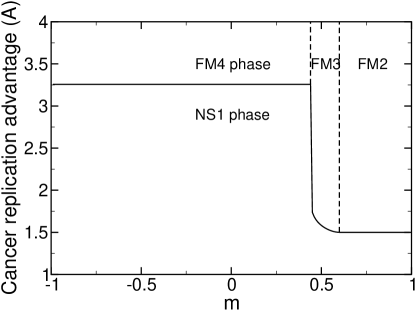
Figure 3: A phase diagram corresponding to the immune control of cancer is shown. We use $\gamma=1$, $B=1$, $M_{0}=0.9$, and $M_{b}=0.54$. The cancer replication advantage required to escape immune system control decreases as the Hamming distance between the cancer and the self decreases, $m\to 1$. Three of the four selective and one of the two non-selective phases are present for the chosen parameters.

V Discussion and Conclusion

We have used the Eigen model to consider the interaction of a virus or cancer with a drug or the immune system. One can also use the parallel model to represent the replication dynamics of the virus or the cancer. This would be an interesting application of our formalism.

Another application of the formalism would be to consider explicitly the degradation induced by multi-drug cocktails. That is, one would consider one peak to represent the preferred virus genome and $K-1$ degradation peaks to represent the $K-1$ drugs. We note that in the general case, the $y_{i}$ parameters depend on the explicit location of the drug degradation peaks, not simply the distance between them. Results from this application of the formalism could be quite illuminating as regards the evolution of multi-drug resistance.

In conclusion, we have solved two common evolution models with general fitness, or replication and degradation rate, landscapes that depend on the Hamming distances from several fitness peaks. Why is this important? First, we have solved the microscopic models, rather than assuming a phenomenological macroscopic model. As is known in statistical mechanics, a phenomenological model may not always detect the fine structure of critical phenomena. Second, approximate or numerical solutions, while useful, do not always explicitly demonstrate the essence of the phenomenon. With analytical solutions, the essence of phenomenon is transparent. Third, we have derived the first path integral formulation of the Eigen model. This formulation may prove useful in other studies of this model of molecular evolution.

Our results for cancer are a case in point. There are four stable selective phases and two stable non-selective phases. These results may help to shed light on the, at present, poorly understood phenomena of interaction with the immune system, and on why the immune response to cancer and to viruses differs in important ways. These phases could well also be related to the different stages, or grades, through which tumors typically progress.

Our results are a first step toward making the connection with evolution on rugged fitness landscapes, landscapes widely accepted to be accurate depictions of nature. We have applied our solution of these microscopic complex adaptive systems to model four situations in biology: how a virus interacts with drug, how an adaptable virus interacts with a drug, the problem of original antigenic sin Deem and Lee (2003), and immune system control of a proliferating cancer.

Appendix

In this section, we derive the path integral representation for the solution to the Eigen model. For simplicity, we show the derivation for the $K=1$ case. To our knowledge, this is the first path integral expression representation of the solution to the Eigen model. This path integral representation allows us to make strong analytic progress. We start from the quantum representation of the Eigen model Saakian and Hu (2004a); Saakian et al. (2004). The Hamiltonian is given by

$$-H = \sum_{l=0}^{N}Ne^{-\gamma}\left(\frac{\gamma}{N}\right)^{l}\sum_{1\leq i_{1}<i_{2}<\ldots<i_{l}\leq N}\sigma_{i_{1}}^{x}\sigma_{i_{2}}^{x}\ldots\sigma_{i_{l}}^{x}$$ (45)

$$\times f_{0}(\sigma^{z})-Nd_{0}(\sigma^{z})$$

$$\approx Ne^{-\gamma}e^{(\gamma/N)\sum_{i}\sigma_{i}^{x}}f_{0}(\sigma^{z})-Nd_{0}(\sigma^{z})\ ,$$

where we have used the fact that with $\gamma/N$ small, we need to consider only $l\ll N$ spin flips. The partition function is decomposed by a Trotter factorization:

$$Z = Tre^{-\beta H}$$ (46)

$$= Tr\langle S_{1}|e^{-\beta H/L}|S_{2}\rangle\langle S_{2}|e^{-\beta H/L}|S_{3}\rangle\ldots$$

$$\times\langle S_{L}|e^{-\beta H/L}|S_{1}\rangle\ .$$

Here

$$\langle S_{l-1}|e^{-\beta H/L}|S_{l}\rangle$$ (47)

$$= \langle S_{l-1}|e^{(\beta N/L)\bigg{[}e^{-\gamma}e^{(\gamma/N)\sum_{i}\sigma_{i}^{x}}f_{0}(\sigma^{z})-d_{0}(\sigma^{z})\bigg{]}}|S_{l}\rangle$$

$$= \langle S_{l-1}|I+\frac{\beta N}{L}\bigg{[}e^{-\gamma}e^{(\gamma/N)\sum_{i}\sigma_{i}^{x}}f_{0}(\sum_{n}s_{n}^{l}/N)$$

$$-d_{0}(\sum_{n}s_{n}^{l}/N)\bigg{]}|S_{l}\rangle\ .$$

We use the notation $M_{l}=\sum_{n}s_{n}^{l}/N$. We find

$$\alpha_{l} = \langle S_{l-1}|I+\frac{\beta N}{L}e^{-\gamma}f_{0}(\sum_{n}s_{n}^{l}/N)e^{(\gamma/N)\sum_{i}\sigma_{i}^{x}}$$ (48)

$$-\frac{\beta N}{L}d_{0}(\sum_{n}s_{n}^{l}/N)|S_{l}\rangle$$

$$= \langle S_{l-1}|S_{l}\rangle\left[1-\frac{\beta N}{L}d_{0}(M_{l})\right]$$

$$+\frac{\beta Ne^{-\gamma}}{L}f_{0}(M_{l})e^{B\sum_{n}(s^{l-1}_{n}s^{l}_{n}-1)}\ ,$$

where $e^{-2B}=\gamma/N$. We thus find

$$\alpha_{l}=\Delta(d_{l})\left[1-\frac{\beta N}{L}d_{0}(M_{l})\right]+\frac{\beta N}{L}e^{-\gamma}f_{0}(M_{l})e^{Bd_{l}}\ ,$$ (49)

where $d_{l}=\sum_{n}(s^{l-1}_{n}s^{l}_{n}-1)$. To represent this in path integral form, we consider

$$\frac{1}{(2\pi)^{2}}\int dhdmd\psi e^{\Delta tNe^{-\gamma}f_{0}(M_{l})e^{Bm}e^{-\psi m}-\Delta tNd_{0}(M_{l})}$$ (50)

$$\times e^{\psi d-h(m-d)}$$

$$= \frac{1}{2\pi}\int dhdm\bigg{[}\delta(d)e^{-\Delta tNd_{0}(M_{l})}+\Delta tNe^{-\gamma}f_{0}(M_{l})$$

$$\times e^{Bm}\delta(m-d)\bigg{]}e^{-h(m-d)}+O[(\Delta t)^{2}]$$

$$= \int dm\bigg{[}\delta(d)\delta(m-d)e^{-\Delta tNd_{0}(M_{l})}+\Delta tNe^{-\gamma}f_{0}(M_{l})$$

$$\times e^{Bm}\delta(m-d)\delta(m-d)\bigg{]}$$

$$= \delta(d)e^{-\Delta tNd_{0}(M_{l})}+\Delta tNe^{-\gamma}f_{0}(M_{l})e^{Bd}\delta(0)$$

$$= \delta(0)\left[\Delta(d)e^{-\Delta tNd_{0}(M_{l})}+\Delta tNe^{-\gamma}f_{0}(M_{l})e^{Bd}\right]\ ,$$

where $\Delta t=\beta/L$. We note that, had we used a Fourier representation of the delta function on the finite domain $[-A/2,A/2]$, instead of the infinite domain $(-\infty,\infty)$, the expression $2\pi\delta(0)$ simply becomes $A$; moreover such a finite representation of the delta function is a sufficiently accurate representation of the $\Delta(d_{l})$ constraint when $A\gg N$. Ignoring the constant prefactor $\delta(0)$ terms, we can write the full partition function as

$$Z = Tr\int{\cal D}\psi{\cal D}h{\cal D}m$$ (51)

$$\times e^{(\beta N/L)\sum_{l}\left[e^{-\gamma}f_{0}(M_{l})e^{Bm_{l}}e^{-\psi_{l}m_{l}}-d_{0}(M_{l})\right]}$$

$$\times e^{\sum_{l}\psi_{l}d_{l}+(\beta N/L)\sum_{l}\left[-h_{l}m_{l}+h_{l}d_{l}\right]}\ .$$

We now introduce the integral representation of the constraint $\delta[(\beta/L)(NM_{l}-\sum_{n}s^{l}_{n})]$. After rescaling $Bm_{l}\to m_{l}$, $h_{l}\to Bh_{l}$ we find

$$Z = Tr\int{\cal D}\psi{\cal D}h{\cal D}m{\cal D}H{\cal D}Me^{(\beta N/L)\sum_{l}[e^{-\gamma}f_{0}(M_{l})e^{m_{l}}}$$

$$\times e^{e^{-\psi_{l}m_{l}/B}-d_{0}(M_{l})-h_{l}m_{l}-H_{l}M_{l}]}$$

$$\times e^{(\beta/L)\sum_{l}H_{l}\sum_{n}s^{l}_{n}+\sum_{l}(\psi_{l}+\beta NBh_{l}/L)\sum_{n}(s^{l-1}_{n}s^{l}_{n}-1)}\ .$$

We note by an expansion of the $\exp[(\beta N/L)e^{-\gamma}f_{0}(M_{l})e^{m_{l}}\exp(-\psi_{l}m_{l}/B)]=$
$\sum_{k_{l}=0}^{\infty}[(\beta N/L)e^{-\gamma}f_{0}(M_{l})e^{m_{l}}]^{k_{l}}\exp(-k_{l}\psi_{l}m_{l}/B)/k_{l}!$ term in Eq. (LABEL:a9) to first order in $\beta N/L$ that the integral over $\psi_{l}$ gives nothing more than $\delta(-k_{l}m_{l}/B+d_{l})$ for $k_{l}=0,1$. This condition, however, is already enforced by the $h_{l}$ field when $k_{l}=1$ and by the $m_{l}$ field when $k_{l}=0$ if we take as a rule to disallow mutations when $h_{l}=0$. We can, thus, remove the integral over $\psi$, removing the $\delta(0)$ that we anticipated, to find

$$Z = \int{\cal D}h{\cal D}m{\cal D}H{\cal D}Me^{(\beta N/L)\sum_{l}[e^{-\gamma}f_{0}(M_{l})e^{m_{l}}-d_{0}(M_{l})}$$ (53)

$$\times e^{-h_{l}m_{l}-H_{l}M_{l}]}Q\ ,$$

where

$$Q=Tre^{(\beta/L)\sum_{l}H_{l}\sum_{n}s^{l}_{n}+(\beta NB/L)\sum_{l}h_{l}\sum_{n}(s^{l-1}_{n}s^{l}_{n}-1)}F$$

$$\ .$$ (54)

Here $Q$ is the partition function of $N$ 1-$d$ Ising models of length $L$. Here $F$ enforces the constraint of disallowing mutations when $h_{l}=0$: $F=\prod_{l=1}^{L}\Delta\{\Delta(h_{l})[\sum_{n}(s^{l-1}_{n}s^{l}_{n}-1)]\}$. We note that $Q=Q_{1}^{N}$, where $Q_{1}$ is the partition function of one of these models. We are not, at this point, allowed to assume that the $H_{l}$ or $h_{l}$ fields are constant over $l$. Indeed, by Taylor series expanding the first term in Eq. 53 and integrating over $m_{l}$, we find that $h_{l}=0$ or $h_{l}=L/(\beta N)$. For $h_{l}=0$, we disallow mutations, as formalized by $F$. Thus, we can replace $e^{-2B}$ by $\gamma t_{l}/N$, where $t_{l}=0$ if $h_{l}=0$, and $t_{l}=1$ if $h_{l}=L/(\beta N)$. We evaluate the partition function $Q_{1}$ with an ordered product of transfer matrices. To first order in $\beta/L$ the matrix at position $l$ is given by $T_{l}=I+\epsilon_{l}$ where

$$\epsilon_{l} = \left(\begin{array}[]{cc}\frac{\beta H_{l}}{L}&\frac{\gamma t_{l}}{N}\\ \frac{\gamma t_{l}}{N}&-\frac{\beta H_{l}}{L}\end{array}\right)$$ (57)

$$= \left(\begin{array}[]{cc}\frac{\beta H_{l}}{L}&\frac{\beta\gamma h_{l}}{L}\\ \frac{\beta\gamma h_{l}}{L}&-\frac{\beta H_{l}}{L}\end{array}\right)\ .$$ (60)

We find

$$Q_{1} = Tr\prod_{l}T_{l}$$ (61)

$$\sim Tr\prod_{l}e^{\epsilon_{l}}\ .$$

We rescale $h\to h/\gamma$ and $m\to m\gamma$ and take the continuous limit to find

$$Q_{1}=Tr\hat{T}e^{\int_{0}^{\beta}d\beta^{\prime}[\sigma^{z}H(\beta^{\prime})+\sigma^{x}h(\beta^{\prime})]}\ ,$$ (62)

where the operator $\hat{T}$ indicates (reverse) time ordering, and $\beta^{\prime}=\beta(L-l)/L$. We find the form of the partition function to be

$$Z = \int{\cal D}h{\cal D}m{\cal D}H{\cal D}M$$

$$e^{N\int_{0}^{\beta}d\beta^{\prime}[e^{-\gamma}f_{0}(M)e^{\gamma m}-d_{0}(M)-hm-HM]+N\ln Q_{1}}\ .$$

Noting the $N$ prefacing the entire term in the exponential, we take the saddle point. We note that $\delta Q_{1}/\delta H(\beta^{\prime})|_{H(\beta^{\prime})=H,h(\beta^{\prime})=h}=(\beta H/\sqrt{H^{2}+h^{2}})2\sinh(\beta\sqrt{H^{2}+h^{2}})$ and
$\delta Q_{1}/\delta h(\beta^{\prime})|_{H(\beta^{\prime})=H,h(\beta^{\prime})=h}=(\beta h/\sqrt{H^{2}+h^{2}})2\sinh(\beta\sqrt{H^{2}+h^{2}})$. We, thus, find a solution of the saddle point condition to be fields $H,M,h,m$ independent of $\beta$ that maximize

$$\frac{\ln Z}{N} = \beta\bigg{[}f_{0}(M)e^{-\gamma}e^{\gamma m}-d_{0}(M)-hm-HM]$$ (64)

$$+\ln[2\cosh(\beta\sqrt{H^{2}+h^{2}})\bigg{]}\ ,$$

when the fields are averaged over a range $\Delta\beta=O(1/N)$ by the saddle point limit. In the limit of large $\beta$, we find

$$\frac{\ln Z}{\beta N} = \max_{M,H,m,h}\bigg{[}f_{0}(M)e^{-\gamma}e^{\gamma m}-d_{0}(M)-hm-HM$$ (65)

$$+(H^{2}+h^{2})^{1/2}\bigg{]}\ .$$

One can also derive Eq. (65) by means of a series expansion in $\beta$, a “high temperature” expansion.

The generalization of the path integral representation to the multiple-peak Eigen case proceeds as in the parallel case. One introduces $K$ fields for the magnetizations, $M^{k}$, and $K$ fields enforcing the constraint, $H^{k}$. One also finds in the linear field part of the Ising model the sum $\sum_{k=1}^{K}H_{l}^{k}\sum_{n}v^{k}_{n}s^{l}_{n}$ instead of simply $H_{l}\sum_{n}s^{l}_{n}$. The definition of the $y_{i}$ and the $\alpha_{ik}$ allows one to rewrite this in the form that leads to Eq. (7) or (24).

References

- Wright (1931) S. Wright, Genetics 16, 97 (1931).
- Kauffmann and Levin (1987) S. Kauffmann and S. Levin, J. Theor. Biol. 128, 11 (1987).
- Baake et al. (1997) E. Baake, M. Baake, and H. Wagner, Phys. Rev. Lett. 78, 559 (1997), 79, 1782.
- Saakian and Hu (2004a) D. B. Saakian and C.-K. Hu, Phys. Rev. E 69, 021913 (2004a).
- Saakian and Hu (2004b) D. B. Saakian and C.-K. Hu, Phys. Rev. E 69, 046121 (2004b).
- Eigen (1971) M. Eigen, Naturwissenschaften 58, 465 (1971).
- Eigen et al. (1989) M. Eigen, J. McCaskill, and P. Schuster, Adv. Chem. Phys. 75, 149 (1989).
- Crow and Kimura (1970) J. F. Crow and M. Kimura, An Introduction to Population Genetics Theory (Harper and Row, New York, 1970).
- Messer et al. (2005) P. W. Messer, P. F. Arndt, and M. Lässig, Phys. Rev. Lett. 94, 138103 (2005).
- Saakian et al. (2004) D. B. Saakian, C.-K. Hu, and H. Khachatryan, Phys. Rev. E 70, 041908 (2004).
- Jain and Krug (2005) K. Jain and J. Krug, in Structural approaches to sequence evolution: Molecules, networks and populations, edited by H. R. U. Bastolla, M. Porto and M. Vendruscolo (Springer Verlag, Berlin, 2005), q-bio.PE/0508008.
- Peliti (2002) L. Peliti, Europhys. Lett. 57, 745 (2002).
- Deem and Lee (2003) M. W. Deem and H. Y. Lee, Phys. Rev. Lett. 91, 068101 (2003).
- Tarazona (1992) P. Tarazona, Phys. Rev. A 45, 6038 (1992).
- Baake et al. (1998) E. Baake, M. Baake, and H. Wagner, Phys. Rev. E 57, 1191 (1998).
- Eigen (2002) M. Eigen, Proc. Natl. Acad. Sci. USA 99, 13374 (2002).
- Park and Deem (2004) J. M. Park and M. W. Deem, Physica A 341, 455 (2004).