Incubation period, anti-retroviral therapies, age-structures

Abstract.

With the launch of second line anti-retroviral therapy for HIV infected individuals, there has been an increased expectation on surviving period of people with HIV. We consider previously well-known models in HIV epidemiology where the parameter for incubation period is used as one of the important components to explain the dynamics of the variables. Such models are extended here to explain the dynamics with respect to a given therapy that prolongs life of an HIV infected individual. A deconvolution method is demonstrated for estimation of parameters in the situations when no-therapy and multiple therapies are given to the infected population. The models and deconvolution method are extended in order to study the impact of therapy in age-structured populations. A generalization for a situation when $n-$types of therapies are available is given. Models are demonstrated using hypothetical data and sensitivity of the parameters are also computed.

Abstract.

With the launch of second line anti-retroviral therapy for HIV infected individuals, there has been an increased expectation on surviving period of people with HIV. We consider previously well-known models in epidemiology where the parameter for incubation period is used as one of the important components to explain the dynamics of the variables. Such models are extended here to explain the dynamics with respect to a given therapy that prolongs life of an HIV infected individual. A deconvolution method is demonstrated for estimation of parameters in the situations when no-therapy and multiple therapies are given to the infected population. The models and deconvolution method are extended in order to study the impact of therapy in age-structured populations. A generalization for a situation when $n-$types of therapies are available is given. Models are demonstrated using hypothetical data and sensitivity of the parameters are also computed.

Full Title: Incubation Periods Under Various Anti-Retroviral Therapies In Homogeneous Mixing And Age-Structured Dynamical Models: A Theoretical Approach.

(Accepted in The Rocky Mountain Journal of Mathematics, USA)

AMS subject classifications: 92D30, 44A35, 62A10

1. Preliminaries, Basic ODE Model and Integro-Differential Equations models

With the introduction of second line therapy[53] to the people living with HIV who were already on first line therapy until introduction of second line therapy, there is a further hope to increase the active life of HIV infected individuals. Revised estimates of the people living with HIV are obtained for some countries to address the impact of second line therapy (see, for example[49]). Second line theory is provided after failure to responding to the first line therapy among the infected individuals. Modeling the impact of second line therapy and corresponding extended survival time is complicated because susceptible population can acquire virus from two infected class of populations who are on therapy in addition to the infected population who are without any therapy. However identifying the first line individuals who are no more responding to the first line therapy through surveillance is still a challenging issue in several countries. Difficulties in monitoring and recording HIV infected population who are on first line and second line therapy will also lead to difficulty in estimating parameters of disease progression and disease related mortalities. Disease progression rate and incubation period are related and usually both are taken as reciprocal to each other. Incubation period of HIV infected individuals is also expected to increase since new anti-retroviral therapy policies. The incubation period is generally defined as ‘the time duration between the time a virus or bacteria enters the human body and the time at which clinical clinical symptoms occur’. This duration can vary from case to case depending upon the route through which the virus or bacteria enters the immune system of an individual and in some cases depends upon the age of the infected individual. For chickenpox this duration is 10 - 21 days, for common cold 2 - 5 days, for mumps 12 to 25 days, for SARS a maximum of up to 10 days, for rubella 14 - 21 days, for pertussis 7 - 10 days, and for HIV infection to AIDS 6 months to 10 years or more. The incubation period can be used as a measure of rapidity of the illness after interaction with the virus or bacteria. It is not easy to collect information on the incubation period of infected individuals unless they are monitored. One of the direct ways of estimating the average incubation period of a given virus in the population is by surveillance and followup of the infected individuals until they develop symptoms. All the infected individuals may not be aware of their infection until symptoms appear and followup is subject to the availability of an individual. It might not be possible to follow up individuals in a typical situation, where time taken for the onset of symptoms from the infection is longer, especially if infected individuals are lost to followup. Hence, there are limitations on directly estimating the average incubation period from prospective cohort studies. Nevertheless, the incubation period occupies an important role along with other parameters in modeling the disease spread and understanding the basic reproductive rate. A useful description of various epidemic models, and of estimation of parameters like the incubation period, transmission rates, forces of infections are presented in [3]. The degree of importance of obtaining accurate average incubation periods varies with the incubation period of the disease. This degree of variation causes mathematical models to act sensitively in predicting future burden. Models describing dynamics of disease spread where the incubation period is shorter are less subject for producing misleading results than models for the spread with longer and varying incubation periods. Especially for predicting AIDS, the epidemic models developed, depend heavily on parameters that determine transmission rates of infection from infected to susceptible and on the parameter which explains the average time to progress to AIDS. A review of various modeling approaches and quantitative techniques to estimate the incubation period can be found in [8, 6]. The introduction of anti-retroviral therapies and protease inhibitors during the 1990s in several parts of the world resulted decline in opportunistic infections related to AIDS [41, 9, 11]. As a result of such interventions, the average incubation period was prolonged. There have been attempts to estimate the incubation period that vary due to drug intervention using statistical density functions [4]. The impact of this variation on the HIV dynamics, stability and on basic reproduction number has been investigated [8, 12, 20]. In this section, we first consider an ODE model that explains the dynamics of HIV spread in a population leading to AIDS (see [13]). We then consider a similar model where incubation period is a variable with respect to a given therapy. We address issues of estimating incubation period to be used in such dynamical models and the impact of above mentioned therapies. Various ideas and the outline of this work are given at the end of this section.

Perhaps the most fundamental model for the epidemiology of AIDS is that given by [13, 2, 3], which takes the form

$$\frac{dX}{dt} = \Lambda-\left(\lambda+\mu\right)X,$$

(1.1) $$\frac{dY}{dt} = \lambda X-\left(d+\mu\right)Y,$$

$$\frac{dD_{z}}{dt} = dY-\gamma D_{z}.$$

Here the total population ($N$) is divided into susceptibles ($X$), infectives ($Y$) and individuals with the full blown disease ($D_{z}$). The parameter $\Lambda$ is the input into the susceptible class, which can be defined as the number of births in the population, $\lambda$ is the force of infection, $\mu$ is general (non-AIDS related) mortality, $\gamma$ is disease related mortality and $1/d$ is the average incubation period. Here the incubation period is defined as the duration of time between infection and onset of full blown disease. There are several other constructions of HIV transmission dynamics models

In the models involving the disease progression parameter, it has been assumed that there is an increase in the mean length of life after HIV infection since the availability of therapies for AIDS [37, 38]. There are several works describing the impact of anti-retroviral therapies using data [1, 21, 22, 23, 24, 25, 26, 27, 28, 29, 30, 31, 32, 33, 34, 35, 36, 39, 40, 41, 43] and through models [23, 38, 42, 44, 45]. The time to start ART based on the CD4 count is still debatable. In a recent study on HIV-1 discordant couples [46], it was observed that the incidence rates among early ART couples are lower than than the incidence rates among couples who were given ART at a standard time. Drugs are available which cannot eliminate virus from the body, but are helpful in prolonging the life of an individual by slowing the disease progression (in other words increasing the incubation period). For example, protease inhibitors (say drug 1) facilitate in producing non-infectious virus (only infectious virus participates in new virus production), hence slowing the disease progression; anti-retroviral therapy (say drug 2) blocks virus from interacting with the non-infected cells and hence reduces the infection process within the cell population (see section 5 in [14] and [15] for fuller details); and a combination of the above two drugs (say drug 3) can be more effective by simultaneously combining the function of drug 1 and drug 2. Note that, when model (1.1) was developed, the above described drugs were not available. Information on scale-up of anti-retroviral therapies and related monitoring of individuals can be found elsewhere (for example, see [23, 50, 47, 51]. We assume that once individuals start taking drugs, their average incubation period is prolonged. So, instead of assuming a constant $1/d$, we assume that it varies based on the drug type. Thus we define $1/d_{i}=\int_{\mathbb{R}}z_{i}g(z_{i})dz_{i},$ for $i=0,1,2,3,$ where $i=0$ denotes the without drug scenario, $i=1$ for drug 1, $i=2$ for drug 2 and $i=3$ for drug 3. Here $g$ is the probability density function with a certain parameter set (say $\mathbb{B}$) and $z_{i}$ is a continuous random variable representing the incubation period. Here $z_{i}$ is a real valued function defined on a standard probability space $\left(S,\mathbb{A},P\right)$, where $S$ is the space of elementary events, $\mathbb{A}$ is called a Borel fields, and $P(\mathbb{A})$ is probability of the event $A\in\mathbb{A}.$ So, $z:S\rightarrow\mathbb{R}.$ We can also denote this integral as a Stieltjes integral $\int_{\mathbb{R}}z_{i}dG(z_{i})$, where $G(z)=P(Z<z).$ We further assume without loss of generality that

(1.2) $$\int_{\mathbb{R}}z_{0}dG(z_{0}) < \int_{\mathbb{R}}z_{1}dG(z_{1})\leq z_{2}dG(z_{2})<\int_{\mathbb{R}}z_{3}dG(z_{3}),$$

$$\int_{\mathbb{R}}z_{0}dG(z_{0}) < \int_{\mathbb{R}}z_{1}dG(z_{1})>\int_{\mathbb{R}}z_{2}dG(z_{2})<\int_{\mathbb{R}}z_{3}dG(z_{3}).$$

(In the next section, we will give a detailed estimation procedure for $\mathbb{B}.$) Applying these varying incubation periods, model (1.1) is modified as follows:

$$\frac{dX}{dt} = \Lambda-\left(\lambda_{0}+\lambda_{1}+\lambda_{2}+\lambda_{3}+\mu\right)X,$$

$$\frac{dY_{0}}{dt} = \lambda_{0}X-\left\{\left(\int_{\mathbb{R}}z_{0}dG(z_{0})\right)^{-1}+\mu\right\}Y_{0},$$

$$\frac{dY_{1}}{dt} = \lambda_{1}X-\left\{\left(\int_{\mathbb{R}}z_{1}dG(z_{1})\right)^{-1}+\mu\right\}Y_{1},$$

$$\frac{dY_{2}}{dt} = \lambda_{2}X-\left\{\left(\int_{\mathbb{R}}z_{2}dG(z_{2})\right)^{-1}+\mu\right\}Y_{2},$$

$$\frac{dY_{3}}{dt} = \lambda_{3}X-\left\{\left(\int_{\mathbb{R}}z_{3}dG(z_{3})\right)^{-1}+\mu\right\}Y_{3},$$

$$\frac{dD_{z_{0}}}{dt} = \left(\int_{\mathbb{R}}z_{0}dG(z_{0})\right)^{-1}Y_{0}-\gamma_{0}D_{z_{0}},$$

(1.3) $$\frac{dD_{z_{1}}}{dt} = \left(\int_{\mathbb{R}}z_{1}dG(z_{1})\right)^{-1}Y_{1}-\gamma_{1}D_{z_{1}},$$

$$\frac{dD_{z_{2}}}{dt} = \left(\int_{\mathbb{R}}z_{2}dF(z_{2})\right)^{-1}Y_{2}-\gamma_{2}D_{z_{2}},$$

$$\frac{dD_{z_{3}}}{dt} = \left(\int_{\mathbb{R}}z_{3}dG(z_{3})\right)^{-1}Y_{3}-\gamma_{3}D_{z_{3}},$$

where $Y_{0},Y_{1},Y{}_{2}$ and $Y_{3}$ are variables for infectives, $D_{z_{0}},D_{z_{1}},D_{z_{2}}$ and $D_{z_{3}}$ are variables for individuals with the full blown disease, $\lambda_{0},\lambda_{1},\lambda_{2}$ and $\lambda_{3}$and $\gamma_{0},\gamma_{1},\gamma_{2}$ and $\gamma_{3}$ are variables for disease related mortality for no-drug, drug 1, drug 2 and drug 3 respectively. See Figure 1.1 describing the flows in the model eq (1.3). General mortality and disease-related mortality are incorporated in to the model to demonstrate the basic structure of the model, and our aim here is to estimate $\mathbb{B}$ and thus to estimate $\int_{\mathbb{R}}z_{i}dG(z_{i})$ for all $i$ such that simulations of the model are performed. In model (1.3), the total population $N=X+Y_{0}+Y_{1}+Y_{2}+Y_{3}+D_{z_{0}}+D_{z_{1}}+D_{z_{2}}+D_{z_{3}}$ satisfies

$$\frac{dN}{dt} = \Lambda-\mu X+\mu\sum_{i=0}^{i=3}Y_{i}-\sum_{i=0}^{3}\gamma_{i}D_{z_{i}}.$$

Figure 1.1. Schematic diagram explaining the flow of infected individuals without therapy to individuals who are on therapy.

Estimation of parameters for the varying incubation periods is important for understanding the impact of drugs in prolonging the onset of disease and thus to prolong the life. The set $\mathbb{B}$ will also be useful in obtaining varying basic reproductive rates, $R_{0i}$ for all $i=0,1,2,3$. This can be computed as $R_{0i}=\lambda\gamma_{i}\int_{\mathbb{R}}z_{i}dG(z_{i})$ by assuming independence of the impact of various drugs. So far, there is no evidence that $\beta,$ the probability of infecting a susceptible partner changes with the activation of a drug in the body. If we assume this as a constant, then $R_{00}\geq R_{01}\geq$ or $<R_{02}\geq R_{03}.$ $R_{01}<\left\{R_{01},R_{02},R_{03}\right\}$, because individuals are assumed to have longer incubation period due to the effect of drugs. In the absence of clinical evidence, we assume that the impact of drug1 and drug2 follows any one of the following relations: $\int_{\mathbb{R}}z_{1}dG(z_{1})\leq$ or $>\textrm{ }\int_{\mathbb{R}}z_{2}dG(z_{2}).$ Similarly, another important epidemiological measure, the doubling time, $t_{di}$ is obtained as $t_{di}=\ln(2)\int_{\mathbb{R}}z_{i}dG(z_{i})/\left[R_{0i}-1\right].$ Anti-retroviral therapy helps in blocking the virus from interacting with cells and simultaneously providing protease inhibitors helps in producing non-infectious virus. So without loss of generality, it is assumed that the impact of double drug therapy is better than a single drug therapy. If we assume disease related mortality is constant for all $i$ then $\gamma_{i}=\gamma.$ The number of AIDS related deaths in general are high during latter part of the incubation period due to increase in opportunistic infections. In general, over all AIDS related mortality rate in a population is assumed to be higher than the general mortality rate in that population. Where there are $n$ types of drugs available, we write the general form for the above dynamical model as follows:

$$\frac{dX}{dt} = \Lambda-\left(\sum_{I=0}^{n}\lambda_{i}+\mu\right)X,$$

$$\frac{dY_{0}}{dt} = \lambda_{0}X-\left\{\left(\int_{\mathbb{R}}z_{0}dG(z_{0})\right)^{-1}+\mu\right\}Y_{0},$$

$$\vdots \vdots$$

$$\vdots \vdots$$

$$\frac{dY_{n}}{dt} = \lambda_{n}X-\left\{\left(\int_{\mathbb{R}}z_{n}dG(z_{n})\right)^{-1}+\mu\right\}Y_{n},$$

$$\frac{dD_{z_{0}}}{dt} = \left(\int_{\mathbb{R}}z_{0}dG(z_{0})\right)^{-1}Y_{0}-\gamma_{0}D_{z_{0}},$$

(1.4) $$\vdots \vdots$$

$$\vdots \vdots$$

$$\frac{dD_{z_{n}}}{dt} = \left(\int_{\mathbb{R}}z_{n}dG(z_{n})\right)^{-1}Y_{n}-\gamma_{n}D_{z_{n}},$$

As a special case we can consider all the parameters in the above model as Stieltjes integrals and can estimate them using the rigorous procedure explained in the next section. For $n=3$ in the model (1.4), we can deduce the model (1.3). Practically, we do not have a situation where several drugs are available in the market for HIV infected individuals. Hence, the model (1.4) should be treated as a theoretical generalization.

This paper is organized as follows: In section 2, we present contemporary models constructed for understanding transmission dynamics of HIV for policy formulations and corresponding modified disease progression component that captures the impact of therapy, in section 3, we describe in detail the estimation of the set $\mathbb{B}$ for up to three drugs; section 4 gives the corresponding expressions for the conditional probabilities of $N-$drugs. We construct theoretical examples using three functions: Gamma, Logistic and Log-normal in section 5 to demonstrate the method explained in section 3. In section 6 analysis for age-structured populations is described in detail. Overall conclusions are given in section 7. Appendix I gives equations for conditional probability when incubation period for various drug types does not have the monotonicity property. Appendix II gives some more theoretical examples when the incubation period is truncated to the right. Appendix III provides parameter values adopted for numerical simulations and Appendix IV has numerical demonstration of the model outputs and sensitivity of parameters in projecting HIV and AIDS.

2. Contemporary models and Modifications

In this section, we present a contemporary model for HIV epidemic in India [19] and corresponding integro-differential equations. HIV model [19] developed based on Indian data has three components, 1) Model for spread in general population, 2) model for spread in homosexual men (MSM), 3) model for spread in intravenous drug users (IDU). We provide a description of this model and then write corresponding revised model with integro differential equations. The system of differential equations in three models have incorporated dynamics in fourteen compartments: $U(i),$ susceptible population; $V(i),$ sexually transmitted diseases population; $W(i),$ HIV infected; $T(i),$ AIDS in the general population for gender $i$ (say, $i=1$ for male and $i=2$ for female), $U(m),$ susceptible MSM; $V(m),$ sexually transmitted infected MSM;, $W(m),$ HIV infected MSM; $T(m),$ MSM population with AIDS; $U(IDU),$ susceptible intravenous drug users; $W(IDU),$ HIV infected intravenous drug users; $T(IDU),$ intravenous drug users with AIDS. Male susceptible in general population is eligible to acquire virus from $j$ th sub-population ($j=1,$ female married partner; $j=2,$ female casual partner, $j=3,$ commercial sex worker; $j=4,$ through blood transfusions. All the sub-populations are allowed to contribute for the transmission dynamics of HIV and each sub-population is also subject to the risk of acquiring the infection from other sub-population wherever applicable (see [19] for complete description).

The differential equations describing the Indian HIV epidemic model are

$$\begin{array}[]{c}\mbox{General}\\ \mbox{Model}\end{array} \begin{cases}\frac{dU(i)}{dt}&=a_{i}U(i)-U(i)\left(\sum_{j=1}^{4}\frac{b_{ij}V(i)}{N(j)}+\sum_{j=1}^{4}\frac{c_{ij}W(j)}{N(j)}\right)+\phi V(i)\\ \\ \frac{dV(i)}{dt}&=U(i)\sum_{j=1}^{4}\frac{b_{ij}V(i)}{N(j)}-V(i)\sum_{j=1}^{4}\frac{d_{ij}W(j)}{N(j)}-\mu V(i)-\phi V(i)\\ \\ \frac{dW(i)}{dt}&=U(i)\sum_{j=1}^{4}\frac{c_{ij}W(j)}{N(j)}+V(i)\sum_{j=1}^{4}\frac{d_{ij}W(j)}{N(j)}-\\ \\ &\qquad\qquad\qquad\qquad\qquad\qquad\qquad\delta_{i}W(i)-\alpha iW(i)\\ \\ \frac{dT(i)}{dt}&=\alpha_{i}W(i)-\mu_{i}T(i)\end{cases}$$

$$\begin{array}[]{c}\mbox{MSM}\\ \mbox{Model}\end{array} \begin{cases}\frac{dU(m)}{dt}&=a_{m}U(m)-U(m)\left(\frac{b_{m}V(m)}{N(m)}+\frac{c_{m}W(m)}{N(m)}\right)+\phi V(m)\\ \\ \frac{dV(m)}{dt}&=U(m)\frac{b_{m}V(m)}{N(m)}-V(m)\frac{d_{m}W(m)}{N(m)}-\mu V(m)-\phi V(m)\\ \\ \frac{dW(m)}{dt}&=U(m)\frac{c_{m}W(m)}{N(m)}+V(m)\frac{d_{m}W(m)}{N(m)}-\\ \\ &\qquad\qquad\qquad\qquad\qquad\qquad\delta_{m}W(m)-\alpha_{m}W(m)\\ \\ \frac{dT(m)}{dt}&=\alpha_{m}W(m)-\mu_{m}T(m)\end{cases}$$

$$\begin{array}[]{c}\mbox{IDU}\\ \mbox{Model}\end{array} \begin{cases}\frac{dU(IDU)}{dt}&=a_{IDU}U(IDU)-U(IDU)\left(\frac{c_{IDU}W(IDU)}{N(IDU)}\right)+\\ \\ &\qquad\qquad\qquad\qquad\qquad\qquad\qquad\phi V(IDU)\\ \\ \frac{dW(IDU)}{dt}&=U(IDU)\frac{c_{IDU}W(IDU)}{N(IDU)}-\delta_{IDU}W(IDU)-\\ \\ &\qquad\qquad\qquad\qquad\qquad\qquad\qquad\alpha_{IDU}W(IDU)\\ \\ \frac{dT(IDU)}{dt}&=\alpha_{IDU}T(IDU)-\mu_{IDU}T(IDU)\end{cases}$$

where, $N(j)=V(j)+W(j)$ for $j=1,2,3,4$ and $N(m)=V(m)+W(m)$

The corresponding models with flexible incubation periods are

$$\frac{dU(i)}{dt} = a_{i}U(i)-U(i)\left(\sum_{j=1}^{4}\frac{b_{ij}V(i)}{N(j)}+\sum_{k=0}^{3}\sum_{j=1}^{4}\frac{c_{ijk}W(j)}{N(j)}\right)+\phi V(i)$$

$$\frac{dV(i)}{dt} = U(i)\sum_{j=1}^{4}\frac{b_{ij}V(i)}{N(j)}-V(i)\sum_{k=0}^{3}\sum_{j=1}^{4}\frac{d_{ijk}W(j)}{N(j)}-\mu V(i)-\phi V(i)$$

$$\frac{dW_{0}(i)}{dt} = U(i)\sum_{j=1}^{4}\frac{c_{ij0}W(j)}{N(j)}+V(i)\sum_{j=1}^{4}\frac{d_{ij0}W(j)}{N(j)}-$$

$$\qquad\qquad\qquad\qquad\qquad\left\{\left(\int_{\mathbb{R}}z_{0}dG(z_{0})\right)^{-1}+\delta_{i}\right\}W_{0}(i)$$

$$\frac{dW_{1}(i)}{dt} = U(i)\sum_{j=1}^{4}\frac{c_{ij1}W(j)}{N(j)}+V(i)\sum_{j=1}^{4}\frac{d_{ij1}W(j)}{N(j)}-$$

$$\qquad\qquad\qquad\qquad\qquad\left\{\left(\int_{\mathbb{R}}z_{1}dG(z_{1})\right)^{-1}+\delta_{i}\right\}W_{1}(i)$$

$$\frac{dW_{2}(i)}{dt} = U(i)\sum_{j=1}^{4}\frac{c_{ij2}W(j)}{N(j)}+V(i)\sum_{j=1}^{4}\frac{d_{ij2}W(j)}{N(j)}-$$

$$\qquad\qquad\qquad\qquad\qquad\left\{\left(\int_{\mathbb{R}}z_{2}dG(z_{2})\right)^{-1}+\delta_{i}\right\}W_{2}(i)$$

$$\frac{dW_{3}(i)}{dt} = U(i)\sum_{j=1}^{4}\frac{c_{ij3}W(j)}{N(j)}+V(i)\sum_{j=1}^{4}\frac{d_{ij3}W(j)}{N(j)}-$$

$$\qquad\qquad\qquad\qquad\qquad\left\{\left(\int_{\mathbb{R}}z_{3}dG(z_{3})\right)^{-1}+\delta_{i}\right\}W_{3}(i)$$

$$\frac{dT_{z0}(i)}{dt} = \left(\int_{\mathbb{R}}z_{0}dG(z_{0})\right)^{-1}W_{0}(i)-\mu_{0}T_{zo}$$

$$\frac{dT_{z1}(i)}{dt} = \left(\int_{\mathbb{R}}z_{1}dG(z_{1})\right)^{-1}W_{1}(i)-\mu_{1}T_{z1}$$

$$\frac{dT_{z2}(i)}{dt} = \left(\int_{\mathbb{R}}z_{2}dG(z_{2})\right)^{-1}W_{2}(i)-\mu_{1}T_{z1}$$

$$\frac{dT_{z3}(i)}{dt} = \left(\int_{\mathbb{R}}z_{3}dG(z_{3})\right)^{-1}W_{3}(i)-\mu_{3}T_{z3}$$

$$\frac{dU(m)}{dt} = a_{m}U(m)-U(m)\left(\frac{b_{m}V(m)}{N(m)}+\sum_{k=0}^{3}\frac{c_{m}W(m)}{N(m)}\right)+\phi V(m)$$

$$\frac{dV(m)}{dt} = U(m)\frac{b_{m}V(m)}{N(m)}-V(m)\sum_{k=0}^{3}\frac{d_{m}W(m)}{N(m)}-\mu V(m)-\phi V(m)$$

$$\frac{dW_{0}(m)}{dt} = U(m)\frac{c_{m0}W(m)}{N(m)}+V(m)\frac{d_{m0}W(m)}{N(m)}-$$

$$\qquad\qquad\qquad\qquad\qquad\left\{\left(\int_{\mathbb{R}}z_{0}dG(z_{0})\right)^{-1}+\delta_{m}\right\}W_{0}(m)$$

$$\frac{dW_{1}(m)}{dt} = U(m)\frac{c_{m1}W(m)}{N(m)}+V(m)\frac{d_{m1}W(m)}{N(m)}-$$

$$\qquad\qquad\qquad\qquad\qquad\left\{\left(\int_{\mathbb{R}}z_{1}dG(z_{1})\right)^{-1}+\delta_{m}\right\}W_{1}(m)$$

$$\frac{dW_{2}(m)}{dt} = U(m)\frac{c_{m2}W(m)}{N(m)}+V(m)\frac{d_{m2}W(m)}{N(m)}-$$

$$\qquad\qquad\qquad\qquad\qquad\left\{\left(\int_{\mathbb{R}}z_{2}dG(z_{2})\right)^{-1}+\delta_{m}\right\}W_{2}(m)$$

$$\frac{dW_{3}(m)}{dt} = U(m)\frac{c_{m3}W(m)}{N(m)}+V(m)\frac{d_{m3}W(m)}{N(m)}-$$

$$\qquad\qquad\qquad\qquad\qquad\left\{\left(\int_{\mathbb{R}}z_{0}dG(z_{0})\right)^{-1}+\delta_{m}\right\}W_{3}(m)$$

$$\frac{dT_{z0}(m)}{dt} = \left(\int_{\mathbb{R}}z_{0}dG(z_{0})\right)^{-1}W_{0}(m)-\mu_{m}T_{z0}(m)$$

$$\frac{dT_{z1}(m)}{dt} = \left(\int_{\mathbb{R}}z_{1}dG(z_{1})\right)^{-1}W_{1}(m)-\mu_{m}T_{z1}(m)$$

$$\frac{dT_{z2}(m)}{dt} = \left(\int_{\mathbb{R}}z_{2}dG(z_{2})\right)^{-1}W_{2}(m)-\mu_{m}T_{z2}(m)$$

$$\frac{dT_{z3}(m)}{dt} = \left(\int_{\mathbb{R}}z_{3}dG(z_{3})\right)^{-1}W_{3}(m)-\mu_{m}T_{z3}(m)$$

$$\frac{dU(IDU)}{dt} = a_{IDU}U(IDU)-U(IDU)\sum_{k=0}^{3}\left(\frac{c_{IDU,k}W(IDU)}{N(IDU)}\right)+\phi V(IDU)$$

$$\frac{dW_{0}(IDU)}{dt} = U(IDU)\left(\frac{c_{IDU,0}W(IDU)}{N(IDU)}\right)-$$

$$\qquad\qquad\qquad\qquad\qquad\left\{\left(\int_{\mathbb{R}}z_{0}dG(z_{0})\right)^{-1}+\delta_{IDU}\right\}W_{0}(IDU)$$

$$\frac{dW_{1}(IDU)}{dt} = U(IDU)\left(\frac{c_{IDU,1}W(IDU)}{N(IDU)}\right)-$$

$$\qquad\qquad\qquad\qquad\qquad\left\{\left(\int_{\mathbb{R}}z_{1}dG(z_{1})\right)^{-1}+\delta_{IDU}\right\}W_{1}(IDU)$$

$$\frac{dW_{2}(IDU)}{dt} = U(IDU)\left(\frac{c_{IDU,2}W(IDU)}{N(IDU)}\right)-$$

$$\qquad\qquad\qquad\qquad\qquad\left\{\left(\int_{\mathbb{R}}z_{2}dG(z_{2})\right)^{-1}+\delta_{IDU}\right\}W_{2}(IDU)$$

$$\frac{dW_{3}(IDU)}{dt} = U(IDU)\left(\frac{c_{IDU,3}W(IDU)}{N(IDU)}\right)-$$

$$\qquad\qquad\qquad\qquad\qquad\left\{\left(\int_{\mathbb{R}}z_{3}dG(z_{3})\right)^{-1}+\delta_{IDU}\right\}W_{3}(IDU)$$

$$\frac{dT_{z0}(IDU)}{dt} = \left(\int_{\mathbb{R}}z_{0}dG(z_{0})\right)^{-1}W_{0}(IDU)-\mu_{IDU}T_{z0}(IDU)$$

$$\frac{dT_{z1}(IDU)}{dt} = \left(\int_{\mathbb{R}}z_{1}dG(z_{1})\right)^{-1}W_{1}(IDU)-\mu_{IDU}T_{z1}(IDU)$$

$$\frac{dT_{z2}(IDU)}{dt} = \left(\int_{\mathbb{R}}z_{2}dG(z_{2})\right)^{-1}W_{2}(IDU)-\mu_{IDU}T_{z2}(IDU)$$

$$\frac{dT_{z3}(IDU)}{dt} = \left(\int_{\mathbb{R}}z_{3}dG(z_{3})\right)^{-1}W_{3}(IDU)-\mu_{IDU}T_{z3}(IDU)$$

where the variables with suffix $z_{0},$ $z_{2}$, $z_{3}$, $z_{3}$ are corresponding to the impact drug0, drug1, drug2, drug3 respectively. These contemporary models are improvised version of basic models presented in section 1 and are tested to predict accurately the epidemic situation during the era of anti-retroviral therapies.

3. Conditional probabilities

In this section, we will give a detailed procedure to estimate $\mathbb{B}$ through a deconvolution technique. Let $\mathbb{B}$ be split into a collection of four parameter sets say, $\mathbb{B}$=$\left\{B_{0},B_{1},B_{2},B_{3}\right\}$ for the four types of scenarios described in the previous section. Let $H$ be the time of infection and $Z$ be the incubation period, then the time of onset of the disease can be represented as $D=H+Z.$ There have been studies (see for list of references Brookmeyer and Gail (1994)), in which $H$ and $Z$ were assumed independent and $D$ was estimated through convolution. We outline the general idea of convolution and then give the convolution of $H$ and $Z.$ Suppose $(a_{n})$ and $(b_{n})$ are two sequences of numbers over the time period, then

(3.1) $$(a_{n})*(b_{n}) = \sum_{k=0}^{n}a_{n}b_{n-k}$$

where $(a_{n})*(b_{n})$ is the convolution of these sequences with an operator ${}^{\prime}*^{\prime}$. Suppose $a$ and $b$ are mutually independent random variables and let $A_{\mathcal{L}}(x)$ and $B_{\mathcal{L}}(x)$ be their Laplace transformations, then $a+b$ has the Laplace transformation $A_{\mathcal{L}}B_{\mathcal{L}}.$ Since the multiplication of the Laplace transformation is associative and commutative, it follows that $(a_{n})*(b_{n})$ is also associative and commutative. Instead of discrete notation, suppose $a$ and $b$ are continuous and independent with probability density functions $h$ and $g$, then the density of $h+g$ is given by

$$f(s) = \int_{-\infty}^{\infty}h(t-s)g(t)dt=\int_{-\infty}^{\infty}h(t)g(t-s)ds$$

.

Suppose $G(s)=\int_{-\infty}^{s}g(s)ds$, and $F(s)=\int_{-\infty}^{s}f(s)ds$ then

(3.2) $$F(s) = \int_{-\infty}^{\infty}h(t)G(t-s)ds.$$

We call $F$ the convolution of $h$ and $G$. Suppose the above $h$ and $G$ represent the infection density and incubation period distribution function; then the convolution of $h$ and $G$ represents the cumulative number of disease cases reported (or observed), and is given by

(3.3) $$h*G = \int_{-\infty}^{\infty}h(t)G(t-s)ds.$$

This kind of convolution in (3.3) was used to estimate the number of AIDS cases for the first time by [7]. Information on $G$ may not be available for some populations. In such situations, $G$ has been estimated through deconvolution from the information available on $h*G$ and $h$ [16, 17]. In this section we will construct conditional probabilities for each drug type and express the function that maximizes $\mathbb{B}$. These kind of conditional probabilities derived for the drug type were not available earlier for the incubation periods when the total number of reported disease cases were considered. Note that $h*G$ is the cumulative number of disease cases.

Let $X_{0},X_{1},X_{2},...,X_{n-k},...,X_{n-l},...,X_{n-m},...,X_{n}$ be the disease cases available in the time intervals $[U_{i-1},U_{i})$ for $i=0,1,2,...n-k,...n-l,...(n-m)+1,...n+1.$ Suppose $\mathbb{E}$ is the event of diagnosis of disease after the first infection at $T_{0}.$ Let $\mathbb{E}=\left\{E_{0},E_{1},E_{2},E_{3}\right\}$ and $E_{0}$ occurs in the interval $[U_{0},U_{n-k})$, $E_{1}$ (or $E_{2}$) in $[U_{n-k},U_{n-l})$ (or $[U_{n-l},U_{n-m})$) and $E_{3}$ in $[U_{n-m},U_{n}).$ Now $D,$ the cumulative number of disease cases up to time $U_{n},$ can be expressed from (3.3) as follows:

(3.4) $$D\left(U_{0}\leq s\leq U_{n}\right) = \int_{0}^{U_{n-k}}h(t)G(t-s)ds+\int_{U_{n-k}}^{U_{n-l}}h(t)G(t-s)ds$$

$$+\int_{U_{n-l}}^{U_{n-m}}h(t)G(t-s)ds+\int_{U_{n-m}}^{U_{n}}h(t)G(t-s)ds,$$

$D\left(\mathbb{A},\mathbb{B}/U_{n}\right)=\int_{0}^{U_{n-k}}h(t/A_{0})G(t-s/B_{0})ds+\int_{U_{n-k}}^{U_{n-l}}h(t/A_{1})G(t-s/B_{1})ds$

$\qquad\qquad+\int_{U_{n-l}}^{U_{n-m}}h(t/A_{2})G(t-s/B_{2})ds+\int_{U_{n-m}}^{U_{n}}h(t/A_{3})G(t-s/B_{3})ds$.

In the above equation $A_{0},$$A_{1},$ $A_{2}$ and $A_{3}$ are the parameter sets for the $h$ for $drug0$, $drug1$, $drug2$ and $drug3$. An infected individual could fall in to any of the intervals described above, and similarly a full-blown disease diagnosed individual could fall in the same interval, but for a given individual the chronological time of infection would be earlier than that of diagnosis of the disease. $U_{n-k}$ is the time of introduction of drugs after infection at $U_{0}.$ Individuals who were diagnosed on or after $U_{n-k},$ and before $U_{n},$ were taking one of the three drugs. If $E_{1}\in[U_{n-k},U_{n-l})$ and $E_{2}\in[U_{n-l},U_{n-m})$ $Z_{1}<Z_{2}$, otherwise if $E_{1}\in[U_{n-l},U_{n-m})$ and $E_{2}\in[U_{n-k},U_{n-l})$ then and if $E_{1},E_{2}\in[U_{n-k},U_{n-m})$ then $Z_{1}=Z_{2}.$ An individual who was diagnosed with the disease before $U_{n}$ must have developed symptoms in one of the four intervals $[U_{0},U_{n-k})$, $[U_{n-k},U_{n-l})$, $[U_{n-l},U_{n-m})$ and $[U_{n-m},U_{n}).$ Let $E_{j}\in[U_{j-1},U_{j})\subseteq[U_{0},U_{n-k})$, then the conditional probability of the occurrence of $E_{j}$ given $E$ is expressed as

$$P\left(E_{j}/E\right) = P\left(U_{j-1}\leq D\leq U_{j}/D\leq U_{n}\right)$$

$$=\frac{D\left(A_{0},B_{0}/U_{j}\right)-D\left(A_{0},B_{0}/U_{j-1}\right)}{D\left(A_{0},B_{0}/U_{n}\right)}$$

(3.5) $$= \int_{0}^{U_{j}}h(t/A_{0})G(t-s/B_{0})ds.\left[\int_{0}^{U_{n}}h(t/A_{0})G(t-s/B_{0})ds\right]^{-1}$$

$$-\int_{0}^{U_{j-1}}h(t/A_{0})G(t-s/B_{0})ds.\left[\int_{0}^{U_{n}}h(t/A_{0})G(t-s/B_{0})ds\right]^{-1}.$$

If drugs were initiated at $U_{n-k},$ then these conditional probabilities constructed above will change according to the occurrence of $E_{1},E_{2},E_{3}.$ Consider $E_{1}\cap E_{2}=\emptyset.$ Let $E_{k}\in[U_{k-1},U_{k})\subseteq[U_{n-k},U_{n-l})$, and $E_{1}\in[U_{n-k},U_{n-l})$, then

$$P\left(E_{k}/E\right) = P\left(U_{k-1}\leq D\leq U_{k}/D\leq U_{n}\right)$$

$$=\frac{D\left(A_{1},B_{1}/U_{k}\right)-D\left(A_{1},B_{1}/U_{k-1}\right)}{D\left(A_{1},B_{1}/U_{n}\right)}$$

(3.6) $$= \int_{0}^{U_{k}}h(t/A_{1})G(t-s/B_{1})ds.\left[\int_{0}^{U_{n}}h(t/A_{1})G(t-s/B_{1})ds\right]^{-1}$$

$$-\int_{0}^{U_{k-1}}h(t/A_{1})G(t-s/B_{1})ds.\left[\int_{0}^{U_{n}}h(t/A_{1})G(t-s/B_{1})ds\right].^{-1}$$

Suppose $E_{k}\in[U_{k-1},U_{k})\subseteq[U_{n-k},U_{n-l})$, and $E_{2}\in[U_{n-k},U_{n-l})$ i.e a situation when $Z_{1}>Z_{2}$, then

(3.7) $$P\left(E_{k}/E\right) = \int_{0}^{U_{k}}h(t/A_{2})G(t-s/B_{2})ds.\left[\int_{0}^{U_{n}}h(t/A_{2})G(t-s/B_{2})ds\right]^{-1}$$

$$-\int_{0}^{U_{k-1}}h(t/A_{2})G(t-s/B_{2})ds.\left[\int_{0}^{U_{n}}h(t/A_{2})G(t-s/B_{2})ds\right]^{-1}.$$

Let $E_{l}\in[U_{l-1},U_{l})\subseteq[U_{n-l},U_{n-m})$, and $E_{2}\in[U_{n-l},U_{n-m}),$ then

$$P\left(E_{l}/E\right) = P\left(U_{l-1}\leq D\leq U_{l}/D\leq U_{n}\right)$$

$$=\frac{D\left(A_{2},B_{2}/U_{l}\right)-D\left(A_{2},B_{2}/U_{l-1}\right)}{D\left(A_{2},B_{2}/U_{n}\right)}$$

(3.8) $$= \int_{0}^{U_{l}}h(t/A_{2})G(t-s/B_{2})ds.\left[\int_{0}^{U_{n}}h(t/A_{2})G(t-s/B_{2})ds\right]^{-1}$$

$$-\int_{0}^{U_{l-1}}h(t/A_{2})G(t-s/B_{2})ds.\left[\int_{0}^{U_{n}}h(t/A_{2})G(t-s/B_{2})ds\right].^{-1}$$

Suppose $E_{l}\in[U_{l-1},U_{l})\subseteq[U_{n-l},U_{n-m})$, and $E_{1}\in[U_{n-l},U_{n-m})$ i.e a situation when $Z_{1}>Z_{2},$ then

(3.9) $$P\left(E_{l}/E\right) = \int_{0}^{U_{l}}h(t/A_{1})G(t-s/B_{1})ds.\left[\int_{0}^{U_{n}}h(t/A_{1})G(t-s/B_{1})ds\right]^{-1}$$

$$-\int_{0}^{U_{l-1}}h(t/A_{1})G(t-s/B_{1})ds.\left[\int_{0}^{U_{n}}h(t/A_{1})G(t-s/B_{1})ds\right]^{-1}.$$

Now consider $E_{1}=E_{2}\in[U_{p-1},U_{p})\subseteq[U_{n-k},U_{n-m}),$ i.e. $Z_{1}=Z_{2},$ then the conditional probabilities contain the same parameter sets. In this situation,

(3.10) $$P\left(E_{p}/E\right) = \int_{0}^{U_{p}}h(t/A_{1})G(t-s/B_{1})ds.\left[\int_{0}^{U_{n}}h(t/A_{1})G(t-s/B_{1})ds\right]^{-1}$$

$$-\int_{0}^{U_{p-1}}h(t/A_{1})G(t-s/B_{1})ds.\left[\int_{0}^{U_{n}}h(t/A_{1})G(t-s/B_{1})ds\right]^{-1}.$$

Since $Z_{3}>Z_{0},Z_{1},Z_{2}$, suppose $E_{3}\in[U_{m-1},U_{m})\subseteq[U_{n-m},U_{n}]$, then

$$P\left(U_{m-1}\leq D\leq U_{m}/D\leq U_{n}\right)=\frac{D\left(A_{3},B_{3}/U_{m}\right)-D\left(A_{3},B_{3}/U_{m-1}\right)}{D\left(A_{3},B_{3}/U_{n}\right)}.$$

Therefore,

(3.11) $$P\left(E_{m}/E\right) = \int_{0}^{U_{m}}h(t/A_{3})G(t-s/B_{3})ds.\left[\int_{0}^{U_{n}}h(t/A_{3})G(t-s/B_{3})ds\right]^{-1}$$

$$-\int_{0}^{U_{m-1}}h(t/A_{3})G(t-s/B_{3})ds.\left[\int_{0}^{U_{n}}h(t/A_{3})G(t-s/B_{3})ds\right]^{-1}$$

The above conditional probabilities $P\left(E_{j}/E\right),P\left(E_{k}/E\right),$ $P\left(E_{l}/E\right),$ $P\left(E_{p}/E\right)$ and $P\left(E_{m}/\mathbb{E}\right)$ are the probabilities associated with the intervals $[U_{j^{\prime}-1},U_{j^{\prime}})$ $,[U_{k^{\prime}-1},U_{k^{\prime}}),$ $[U_{l^{\prime}-1},U_{l^{\prime}}),[U_{p^{\prime}-1},U_{p^{\prime}})$ and $[U_{m^{\prime}-1},U_{m^{\prime}})$ for the ranges of $j,k,l,p$ and $m$ defined above. Since, $X_{0},X_{1},X_{2},...,X_{n-k},...,$$X_{n-l},...,X_{n-m},...,X_{n}$ are mutually exclusive, we assume they follow a parametric distribution with the above probabilities are mutually exclusive, so we assume they follow the multinomial property of the distribution of the values in the time intervals and the above conditional probabilities. Then the likelihood functions corresponding to the event set $\mathbb{E}$ are $L_{0}\left(\mathbb{A},\mathbb{B}/P_{j}\right)=$$\prod_{j^{\prime}=1}^{n-k}$ $P_{j}\left(\mathbb{A},\mathbb{B}/T_{j^{\prime}}\right)$, $L_{1(2)}\left(\mathbb{A},\mathbb{B}/P_{k}\right)=\prod_{k^{\prime}=n-k}^{n-l}$$P_{k^{\prime}}\left(\mathbb{A},\mathbb{B}/T_{k^{\prime}}\right)$, $L_{2(1)}\left(\mathbb{A},\mathbb{B}/P_{l^{\prime}}\right)=\prod_{l^{\prime}=n-l}^{n-m}$ $P_{l^{\prime}}\left(\mathbb{A},\mathbb{B}/T_{l^{\prime}}\right)$, $L_{1=2}\left(\mathbb{A},\mathbb{B}/P_{p}\right)$ $=\prod_{p^{\prime}=n-k}^{n-m}P_{p^{\prime}}\left(\mathbb{A},\mathbb{B}/T_{p^{\prime}}\right)$ and $L_{3}\left(\mathbb{A},\mathbb{B}/P_{m}\right)=\prod_{m^{\prime}=n-m}^{n}P_{m^{\prime}}\left(\mathbb{A},\mathbb{B}/T_{m^{\prime}}\right).$ Here $P_{\bullet}=P(E_{\bullet}/\mathbb{E}).$ We estimate $\mathbb{A}$ by fitting an infection curve from the incidence data and we then estimate $\mathbb{B}$ by maximizing the likelihood functions expressed above. The best estimate of $\mathbb{A}$ could be information for initial values of $X$ and $Y$ in the model (1.3). Using the corresponding estimate of $\mathbb{B}$, we obtain $\int_{\mathbb{R}}z_{i}dF(z_{i}).$ In such situations, the above likelihood functions would be $L_{0}=\prod_{j^{\prime}=0}^{n-k}P_{j}^{T_{j^{\prime}}},$ $L_{1(2)}=\prod_{k^{\prime}=n-k}^{n-l}P_{k}^{T_{k^{\prime}}},$$L_{2(1)}=\prod_{l^{\prime}=n-l}^{n-m}P_{l}^{T_{l^{\prime}}},$ $L_{1=2}=\prod_{p^{\prime}=n-k}^{n-m}P_{p}^{T_{p^{\prime}}}$ and $L_{3}=$ $\prod_{m^{\prime}=n-m}^{n}P_{m}^{T_{m^{\prime}}}.$

4. Generalization for multiple drug impact

In this section, expressions for the conditional probabilities are presented when multiple drugs are administrated in the population. Refer to the sections 2 and 3 for introduction on the role of various drugs and refer to the section 4 for basic formulations of conditional probabilities when there are three types of drugs to prolong the incubation period and without any drug situation that would not alter natural process of disease progression. Modeling for the situation corresponding to no drug is highly relevant for those countries where surveillance and diagnosis of infections are not complete and several individuals with HIV are not taking drugs. Let $N=\left\{N_{0},N_{1},N_{2},\right.$ $\left....,N_{N}\right\}$ be the number of available drugs and $Z=\left\{Z_{0},Z_{1},Z_{2},...,Z_{N}\right\}$ be their corresponding incubation periods. Further let $Z_{0}<Z_{1}<Z_{2}<,...,<Z_{N}$ and $\mathbb{A}$ and $\mathbb{B}$ be their parametric sets. Then

(4.1) $$D\left(\mathbb{A},\mathbb{B}/U_{N_{N}}\right) = \int_{0}^{U_{N_{0}}}h(t/A_{N_{0}})G(t-s/B_{N_{0}})ds$$

$$+\int_{U_{N_{0}}}^{U_{N_{1}}}h(t/A_{N_{1}})G(t-s/B_{N_{1}})ds$$

$$\cdots+\int_{U_{N_{N-1}}}^{U_{N_{N}}}h(t/A_{N_{N}})G(t-s/B_{N_{N}})ds.$$

Now, $P\left(E_{N_{i}}/E\right)=P\left(U_{N_{i-1}}\leq D\leq U_{N_{i}}/D\leq U_{N_{N}}\right)$ and $L_{N_{i}}$ (for some $i$) can be computed as follows:

(4.2) $$P\left(E_{N_{i}}/E\right) = \int_{0}^{U_{N_{i}}}h(t/A_{N_{i}})G(t-s/B_{N_{i}})ds\times$$

$$\left[\int_{0}^{U_{N_{N}}}h(t/A_{N_{N}})G(t-s/B_{N_{N}})ds\right]^{-1}$$

$$-\int_{0}^{U_{N_{i-1}}}h(t/A_{N_{i-1}})G(t-s/B_{N_{i-1}})ds\times$$

$$\left[\int_{0}^{U_{N_{N}}}h(t/A_{N_{N}})G(t-s/B_{N_{N}})ds\right].^{-1}$$

$L_{N_{i}}=\prod_{j=N_{i-1}}^{N_{i}}P_{j}^{T_{j}}$ is maximized for the set $\left[A_{i},B_{i}\right]$ by the procedure explained in the previous section. We will obtain $N$ sets of $\left[\mathbb{A},\mathbb{B}\right]$ values, and the corresponding likelihood values are $L_{N_{1}},L_{N_{2}},L_{N_{3}},...,L_{N_{N}}.$ In the above, we have assumed monotonicity of $(Z_{i})$ to arrive at (4.2). If the $(Z_{i})$ values are not monotonic then the various conditional probabilities can be constructed as explained in the previous section. There we explained the general expression when there were a finite number of drugs available on the market. A detailed construction of various conditional probabilities is not necessary for the purpose of the present section (for details see Appendix I). When the $Z_{i}s$ are not monotonic, and if they follow some order, say for example, $Z_{0}>Z_{1}<Z_{2}>...<Z_{N},$ then the conditional probabilities can be constructed in the same way as equations (3.7e3.9) were. Suppose $(Z_{p})$ are equal for each $p$, then there will be two scenarios arising: one for before drug intervention and one after drug intervention. For this situation, the likelihood equation is $L_{N_{p}}=\prod_{p=N_{p-1}}^{N_{p}}P_{p}^{T_{p}}$ where $P\left(E_{N_{p}}/E\right),{}$ is given as follows:

(4.3) $$P\left(E_{N_{p}}/E\right) = \int_{0}^{U_{N_{p}}}h(t/A_{N_{p}})G(t-s/B_{N_{p}})ds\times$$

$$\left[\int_{0}^{U_{N_{N}}}h(t/A_{N_{N}})G(t-s/B_{N_{N}})ds\right]^{-1}$$

$$-\int_{0}^{U_{N_{p-1}}}h(t/A_{N_{p-1}})G(t-s/B_{N_{p-1}})ds\times$$

$$\left[\int_{0}^{U_{N_{N}}}h(t/A_{N_{N}})G(t-s/B_{N_{N}})ds\right].$$

5. Theoretical examples

In this section, we show some examples of the likelihood function constructed in the previous section, to estimate $\mathbb{A},\textrm{ and }\mathbb{B}.$ Let $h(s)$ follow a quadratic exponential and $\mathbb{B}$ follow a) a gamma function, and b) a logistic function. Infections in most of the countries started declining after the availability of antiretroviral therapies [9, 11], and incidence in the recent period was found to be stable in some countries like India [19]. This motivated us to choose a quadratic exponential to represent $h(s)$, namely $h(s)=exp(\alpha_{1}s^{2}+\alpha_{2}s+\alpha_{3})$ for all $-\infty<\alpha_{1},\alpha_{2},\alpha_{3}<\infty$. A quadratic exponential function has been shown to be a good model for representing the above declines in the incidence rates [17]. The incubation period for AIDS is large as well as variable, therefore, functions like the gamma, Weibull and logistic can mimic several shapes to fit the incubation period data depending on their parameter values. Such well-known functions were used by many researchers for modeling the incubation period of AIDS. We now demonstrate the application of such functions for the theory explained in section 2.

5.1. Example 1: Gamma function. If $\omega>0$ is the parameter and $\Gamma(\omega)$ is the complete distribution function, then the incomplete gamma distribution, $G(\omega;t_{j})=\frac{1}{\Gamma(\omega)}\int_{0}^{t_{j}}e^{-x}x^{\omega-1}dx,$ for $a\geq 0,t_{j}\geq 0$ and $a+t_{j}\neq 0$

From the conditional probability equations from (3.5) to (3.11), and the likelihood equations explained in the later part of section 3, the following are the likelihood equations without a drug and for with three types of drugs:

(5.1) $$L_{0}\left(\alpha_{1},\alpha_{2},\alpha_{3};\omega/P_{j}\right) = \prod_{j}a_{1}(j)a_{2}(j)-\prod_{j}a_{1}(j-1)a_{2}(j)$$

where

$$a_{1}(j) = \left[\int_{0}^{u_{j}}e^{\alpha_{1}s^{2}+\alpha_{2}s+\alpha_{3}}\left\{\frac{1}{\Gamma\omega}\int_{0}^{t_{j}}e^{{}_{-(u_{j}-s)}}(u_{j}-s)^{\omega-1}du_{j}\right\}ds\right]^{T_{j}}$$

$$a_{1}(j-1) = \left[\int_{0}^{u_{j-1}}e^{\alpha_{1}s^{2}+\alpha_{2}s+\alpha_{3}}\right.$$

$$\qquad\qquad\left.\times\left\{\frac{1}{\Gamma\omega}\int_{0}^{t_{j-1}}e^{{}_{-(u_{j-1}-s)}}(u_{j-1}-s)^{\omega-1}du_{j-1}\right\}ds\right]^{T_{j}}$$

$$a_{2}(j) = \left[\int_{0}^{u_{n}}e^{\alpha_{1}s^{2}+\alpha_{2}s+\alpha_{3}}\left\{\frac{1}{\Gamma\omega}\int_{0}^{t_{n}}e^{{}_{-(u_{n}-s)}}(u_{n}-s)^{\omega-1}du_{n}\right\}ds\right]^{-T_{j}}$$

(5.2) $$L_{1(2)}\left(\alpha_{1},\alpha_{2},\alpha_{3};\omega/P_{k}\right) = \prod_{k}a_{1}(k)a_{2}(k)-\prod_{k}a_{1}(k-1)a_{2}(k)$$

where

$$a_{1}(k) = \left[\int_{0}^{u_{k}}e^{\alpha_{1}s^{2}+\alpha_{2}s+\alpha_{3}}\left\{\frac{1}{\Gamma\omega}\int_{0}^{t_{k}}e^{{}_{-(u_{k}-s)}}(u_{k}-s)^{\omega-1}du_{k}\right\}ds\right]^{T_{k}}$$

$$a_{1}(k-1) = \left[\int_{0}^{u_{k-1}}e^{\alpha_{1}s^{2}+\alpha_{2}s+\alpha_{3}}\right.{}$$

$$\qquad\qquad\left.\times\left\{\frac{1}{\Gamma\omega}\int_{0}^{t_{k-1}}e^{{}_{-(u_{k-1}-s)}}(u_{k-1}-s)^{\omega-1}du_{k-1}\right\}ds\right]^{T_{k}}$$

$$a_{2}(k) = \left[\int_{0}^{u_{n}}e^{\alpha_{1}s^{2}+\alpha_{2}s+\alpha_{3}}\left\{\frac{1}{\Gamma\omega}\int_{0}^{t_{n}}e^{{}_{-(u_{n}-s)}}(u_{n}-s)^{\omega-1}du_{n}\right\}ds\right]^{-T_{k}}$$

(5.3) $$L_{2(1)}\left(\alpha_{1},\alpha_{2},\alpha_{3};\omega/P_{l}\right) = \prod_{l}a_{1}(l)a_{2}(l)-\prod_{l}a_{1}(l-1)a_{2}(l)$$

where

$$a_{1}(l) = \left[\int_{0}^{u_{l}}e^{\alpha_{1}s^{2}+\alpha_{2}s+\alpha_{3}}\left\{\frac{1}{\Gamma\omega}\int_{0}^{t_{l}}e^{{}_{-(u_{l}-s)}}(u_{l}-s)^{\omega-1}du_{l}\right\}ds\right]^{T_{l}}$$

$$a_{1}(l-1) = \left[\int_{0}^{u_{l-1}}e^{\alpha_{1}s^{2}+\alpha_{2}s+\alpha_{3}}\right.{}$$

$$\qquad\qquad\left.\times\left\{\frac{1}{\Gamma\omega}\int_{0}^{t_{l-1}}e^{{}_{-(u_{l-1}-s)}}(u_{l-1}-s)^{\omega-1}du_{l-1}\right\}ds\right]^{T_{l}}$$

$$a_{2}(l) = \left[\int_{0}^{u_{n}}e^{\alpha_{1}s^{2}+\alpha_{2}s+\alpha_{3}}\left\{\frac{1}{\Gamma\omega}\int_{0}^{t_{n}}e^{{}_{-(u_{n}-s)}}(u_{n}-s)^{\omega-1}du_{n}\right\}ds\right]^{-T_{l}}$$

(5.4) $$L_{1=2}\left(\alpha_{1},\alpha_{2},\alpha_{3};\omega/P_{p}\right) = \prod_{p}a_{1}(p)a_{2}(p)-\prod_{p}a_{1}(p-1)a_{2}(p)$$

where

$$a_{1}(p) = \left[\int_{0}^{u_{p}}e^{\alpha_{1}s^{2}+\alpha_{2}s+\alpha_{3}}\left\{\frac{1}{\Gamma\omega}\int_{0}^{t_{p}}e^{{}_{-(u_{p}-s)}}(u_{p}-s)^{\omega-1}du_{p}\right\}ds\right]^{T_{p}}$$

$$a_{1}(p-1) = \left[\int_{0}^{u_{p-1}}e^{\alpha_{1}s^{2}+\alpha_{2}s+\alpha_{3}}\right.$$

$$\qquad\qquad\left.\times\left\{\frac{1}{\Gamma\omega}\int_{0}^{t_{p-1}}e^{{}_{-(u_{p-1}-s)}}(u_{p-1}-s)^{\omega-1}du_{p-1}\right\}ds\right]^{T_{p}}$$

$$a_{2}(p) = \left[\int_{0}^{u_{n}}e^{\alpha_{1}s^{2}+\alpha_{2}s+\alpha_{3}}\left\{\frac{1}{\Gamma\omega}\int_{0}^{t_{n}}e^{{}_{-(u_{n}-s)}}(u_{n}-s)^{\omega-1}du_{n}\right\}ds\right]^{-T_{p}}$$

(5.5) $$L_{3}\left(\alpha_{1},\alpha_{2},\alpha_{3};\omega/P_{m}\right) = \prod_{m}a_{1}(m)a_{2}(m)-\prod_{m}a_{1}(m-1)a_{2}(m)$$

where

$$a_{1}(m) = \left[\int_{0}^{u_{m}}e^{\alpha_{1}s^{2}+\alpha_{2}s+\alpha_{3}}\left\{\frac{1}{\Gamma\omega}\int_{0}^{t_{m}}e^{{}_{-(u_{m}-s)}}(u_{m}-s)^{\omega-1}du_{m}\right\}ds\right]^{T_{m}}$$

$$a_{1}(m-1) = \left[\int_{0}^{u_{m-1}}e^{\alpha_{1}s^{2}+\alpha_{2}s+\alpha_{3}}\right.$$

$$\qquad\qquad\left.\times\left\{\frac{1}{\Gamma\omega}\int_{0}^{t_{m-1}}e^{{}_{-(u_{m-1}-s)}}(u_{m-1}-s)^{\omega-1}du_{m-1}\right\}ds\right]^{T_{m}}$$

$$a_{2}(m) = \left[\int_{0}^{u_{n}}e^{\alpha_{1}s^{2}+\alpha_{2}s+\alpha_{3}}\left\{\frac{1}{\Gamma\omega}\int_{0}^{t_{n}}e^{{}_{-(u_{n}-s)}}(u_{n}-s)^{\omega-1}du_{n}\right\}ds\right]^{-T_{m}}$$

5.2. Example 2: Logistic function. Suppose $\theta_{1},\theta_{2}$ are parameters and $F(\theta_{1},\theta_{2};t_{j})=\left\{1+e^{-(\frac{t_{j}-\theta_{1}}{\theta_{2}})}\right\}^{-1},$ for $\theta_{1},\theta_{2}>0,$ is the distribution function.

The likelihood equations to obtain the parameters of logistic distribution without drugs and for three types of drugs are as follows:

(5.6) $$L_{0}\left(\alpha_{1},\alpha_{2},\alpha_{3};\theta_{1},\theta_{2}/P_{j}\right) = \prod_{j}a^{\prime}_{1}(j)a^{\prime}_{2}(j)-\prod_{j}a^{\prime}_{1}(j-1)a^{\prime}_{2}(j)$$

where

$$a^{\prime}_{1}(j) = \left[\int_{0}^{u_{j}}e^{\alpha_{1}s^{2}+\alpha_{2}s+\alpha_{3}}\left\{\left\{1+e^{-(\frac{u_{j}-\theta_{1}}{\theta_{2}})}\right\}^{-1}\right\}ds\right]^{T_{j}}$$

$$a^{\prime}_{1}(j-1) = \left[\int_{0}^{u_{j-1}}e^{\alpha_{1}s^{2}+\alpha_{2}s+\alpha_{3}}\left\{\left\{1+e^{-(\frac{u_{j-1}-\theta_{1}}{\theta_{2}})}\right\}^{-1}\right\}ds\right]^{T_{j}}$$

$$a^{\prime}_{2}(j) = \left[\int_{0}^{u_{n}}e^{\alpha_{1}s^{2}+\alpha_{2}s+\alpha_{3}}\left\{\left\{1+e^{-(\frac{u_{n}-\theta_{1}}{\theta_{2}})}\right\}^{-1}\right\}ds\right]^{-T_{j}}$$

(5.7) $$L_{1(2)}\left(\alpha_{1},\alpha_{2},\alpha_{3};\theta_{1},\theta_{2}/P_{k}\right) = \prod_{k}a^{\prime}_{1}(k)a^{\prime}_{2}(k)-\prod_{k}a^{\prime}_{1}(k-1)a^{\prime}_{2}(k)$$

where

$$a^{\prime}_{1}(k) = \left[\int_{0}^{u_{k}}e^{\alpha_{1}s^{2}+\alpha_{2}s+\alpha_{3}}\left\{\left\{1+e^{-(\frac{u_{k}-\theta_{1}}{\theta_{2}})}\right\}^{-1}\right\}ds\right]^{T_{k}}$$

$$a^{\prime}_{1}(k-1) = \left[\int_{0}^{u_{k-1}}e^{\alpha_{1}s^{2}+\alpha_{2}s+\alpha_{3}}\left\{\left\{1+e^{-(\frac{u_{k-1}-\theta_{1}}{\theta_{2}})}\right\}^{-1}\right\}ds\right]^{T_{k}}$$

$$a^{\prime}_{2}(k) = \left[\int_{0}^{u_{n}}e^{\alpha_{1}s^{2}+\alpha_{2}s+\alpha_{3}}\left\{\left\{1+e^{-(\frac{u_{n}-\theta_{1}}{\theta_{2}})}\right\}^{-1}\right\}ds\right]^{-T_{k}}$$

(5.8) $$L_{2(1)}\left(\alpha_{1},\alpha_{2},\alpha_{3};\theta_{1},\theta_{2}/P_{l}\right) = \prod_{l}a^{\prime}_{1}(l)a^{\prime}_{2}(l)-\prod_{l}a^{\prime}_{1}(l-1)a^{\prime}_{2}(l)$$

where

$$a^{\prime}_{1}(l) = \left[\int_{0}^{u_{l}}e^{\alpha_{1}s^{2}+\alpha_{2}s+\alpha_{3}}\left\{\left\{1+e^{-(\frac{u_{l}-\theta_{1}}{\theta_{2}})}\right\}^{-1}\right\}ds\right]^{T_{l}}$$

$$a^{\prime}_{1}(l-1) = \left[\int_{0}^{u_{l-1}}e^{\alpha_{1}s^{2}+\alpha_{2}s+\alpha_{3}}\left\{\left\{1+e^{-(\frac{u_{l-1}-\theta_{1}}{\theta_{2}})}\right\}^{-1}\right\}ds\right]^{T_{l}}$$

$$a^{\prime}_{2}(l) = \left[\int_{0}^{u_{n}}e^{\alpha_{1}s^{2}+\alpha_{2}s+\alpha_{3}}\left\{\left\{1+e^{-(\frac{u_{n}-\theta_{1}}{\theta_{2}})}\right\}^{-1}\right\}ds\right]^{-T_{l}}$$

(5.9) $$L_{1=2}\left(\alpha_{1},\alpha_{2},\alpha_{3};\theta_{1},\theta_{2}/P_{p}\right) = \prod_{p}a^{\prime}_{1}(p)a^{\prime}_{2}(p)-\prod_{p}a^{\prime}_{1}(p-1)a^{\prime}_{2}(p)$$

where

$$a^{\prime}_{1}(p) = \left[\int_{0}^{u_{p}}e^{\alpha_{1}s^{2}+\alpha_{2}s+\alpha_{3}}\left\{\left\{1+e^{-(\frac{u_{p}-\theta_{1}}{\theta_{2}})}\right\}^{-1}\right\}ds\right]^{T_{p}}$$

$$a^{\prime}_{1}(p-1) = \left[\int_{0}^{u_{p-1}}e^{\alpha_{1}s^{2}+\alpha_{2}s+\alpha_{3}}\left\{\left\{1+e^{-(\frac{u_{p-1}-\theta_{1}}{\theta_{2}})}\right\}^{-1}\right\}ds\right]^{T_{p}}$$

$$a^{\prime}_{2}(p) = \left[\int_{0}^{u_{n}}e^{\alpha_{1}s^{2}+\alpha_{2}s+\alpha_{3}}\left\{\left\{1+e^{-(\frac{u_{n}-\theta_{1}}{\theta_{2}})}\right\}^{-1}\right\}ds\right]^{-T_{p}}$$

(5.10) $$L_{3}\left(\alpha_{1},\alpha_{2},\alpha_{3};\theta_{1},\theta_{2}/P_{m}\right) = \prod_{m}a^{\prime}_{1}(m)a^{\prime}_{2}(m)-\prod_{m}a^{\prime}_{1}(m-1)a_{2}(m)$$

where

$$a^{\prime}_{1}(m) = \left[\int_{0}^{u_{m}}e^{\alpha_{1}s^{2}+\alpha_{2}s+\alpha_{3}}\left\{\left\{1+e^{-(\frac{u_{m}-\theta_{1}}{\theta_{2}})}\right\}^{-1}\right\}ds\right]^{T_{m}}$$

$$a^{\prime}_{1}(m-1) = \left[\int_{0}^{u_{m-1}}e^{\alpha_{1}s^{2}+\alpha_{2}s+\alpha_{3}}\left\{\left\{1+e^{-(\frac{u_{m-1}-\theta_{1}}{\theta_{2}})}\right\}^{-1}\right\}ds\right]^{T_{m}}$$

$$a^{\prime}_{2}(m) = \left[\int_{0}^{u_{n}}e^{\alpha_{1}s^{2}+\alpha_{2}s+\alpha_{3}}\left\{\left\{1+e^{-(\frac{u_{n}-\theta_{1}}{\theta_{2}})}\right\}^{-1}\right\}ds\right]^{-T_{m}}$$

5.3. Example 3: Log-normal function. Suppose $\mu\textrm{ and }\sigma$ are parameters and $LNF(\mu,\sigma;t_{j})=\frac{1}{2}\left\{1+erf\left(\frac{\ln x-\mu}{\sigma\sqrt{2}}\right)\right\},$ for $\mu,\sigma>0,$ is the distribution function. (Here $erf\{.\}$ is the error function of the Gaussian function)

The likelihood equations to obtain the parameters of the logistic distribution without drugs and for three types of drugs are as follows:

(5.11) $$L_{0}\left(\alpha_{1},\alpha_{2},\alpha_{3};\mu,\sigma/P_{j}\right) = \prod_{j}a^{\prime\prime}_{1}(j)a^{\prime\prime}_{2}(j)-\prod_{j}a^{\prime\prime}_{1}(j-1)a^{\prime\prime}_{2}(j)$$

where

$$a^{\prime\prime}_{1}(j) = \left[\frac{1}{2}\int_{0}^{u_{j}}e^{\alpha_{1}s^{2}+\alpha_{2}s+\alpha_{3}}\left\{1+erf\left(\frac{\ln x-\mu}{\sigma\sqrt{2}}\right)\right\}ds\right]^{T_{j}}$$

$$a^{\prime\prime}_{1}(j-1) = \left[\frac{1}{2}\int_{0}^{u_{j-1}}e^{\alpha_{1}s^{2}+\alpha_{2}s+\alpha_{3}}\left\{1+erf\left(\frac{\ln x-\mu}{\sigma\sqrt{2}}\right)\right\}ds\right]^{T_{j}}$$

$$a^{\prime\prime}_{2}(j) = \left[\frac{1}{2}\int_{0}^{u_{n}}e^{\alpha_{1}s^{2}+\alpha_{2}s+\alpha_{3}}\left\{1+erf\left(\frac{\ln x-\mu}{\sigma\sqrt{2}}\right)\right\}ds\right]^{-T_{j}}$$

(5.12) $$L_{1(2)}\left(\alpha_{1},\alpha_{2},\alpha_{3};\mu,\sigma/P_{k}\right) = \prod_{k}a^{\prime\prime}_{1}(k)a^{\prime\prime}_{2}(k)-\prod_{k}a^{\prime\prime}_{1}(k-1)a^{\prime\prime}_{2}(k)$$

where

$$a^{\prime\prime}_{1}(k) = \left[\frac{1}{2}\int_{0}^{u_{k}}e^{\alpha_{1}s^{2}+\alpha_{2}s+\alpha_{3}}\left\{1+erf\left(\frac{\ln x-\mu}{\sigma\sqrt{2}}\right)\right\}ds\right]^{T_{k}}$$

$$a^{\prime\prime}_{1}(k-1) = \left[\frac{1}{2}\int_{0}^{u_{k-1}}e^{\alpha_{1}s^{2}+\alpha_{2}s+\alpha_{3}}\left\{1+erf\left(\frac{\ln x-\mu}{\sigma\sqrt{2}}\right)\right\}ds\right]^{T_{k}}$$

$$a^{\prime\prime}_{2}(k) = \left[\frac{1}{2}\int_{0}^{u_{n}}e^{\alpha_{1}s^{2}+\alpha_{2}s+\alpha_{3}}\left\{1+erf\left(\frac{\ln x-\mu}{\sigma\sqrt{2}}\right)\right\}ds\right]^{-T_{k}}$$

(5.13) $$L_{2(1)}\left(\alpha_{1},\alpha_{2},\alpha_{3};\mu,\sigma/P_{l}\right) = \prod_{l}a^{\prime\prime}_{1}(l)a^{\prime\prime}_{2}(l)-\prod_{l}a^{\prime\prime}_{1}(l-1)a^{\prime\prime}_{2}(l)$$

where

$$a^{\prime\prime}_{1}(l) = \left[\frac{1}{2}\int_{0}^{u_{l}}e^{\alpha_{1}s^{2}+\alpha_{2}s+\alpha_{3}}\left\{1+erf\left(\frac{\ln x-\mu}{\sigma\sqrt{2}}\right)\right\}ds\right]^{T_{l}}$$

$$a^{\prime\prime}_{1}(l-1) = \left[\frac{1}{2}\int_{0}^{u_{l-1}}e^{\alpha_{1}s^{2}+\alpha_{2}s+\alpha_{3}}\left\{1+erf\left(\frac{\ln x-\mu}{\sigma\sqrt{2}}\right)\right\}ds\right]^{T_{l}}$$

$$a^{\prime\prime}_{2}(l) = \left[\frac{1}{2}\int_{0}^{u_{n}}e^{\alpha_{1}s^{2}+\alpha_{2}s+\alpha_{3}}\left\{1+erf\left(\frac{\ln x-\mu}{\sigma\sqrt{2}}\right)\right\}ds\right]^{-T_{l}}$$

(5.14) $$L_{1=2}\left(\alpha_{1},\alpha_{2},\alpha_{3};\mu,\sigma/P_{p}\right) = \prod_{p}a^{\prime\prime}_{1}(p)a^{\prime\prime}_{2}(p)-\prod_{p}a^{\prime\prime}_{1}(p-1)a^{\prime\prime}_{2}(p)$$

where

$$a^{\prime\prime}_{1}(p) = \left[\frac{1}{2}\int_{0}^{u_{p}}e^{\alpha_{1}s^{2}+\alpha_{2}s+\alpha_{3}}\left\{1+erf\left(\frac{\ln x-\mu}{\sigma\sqrt{2}}\right)\right\}ds\right]^{T_{p}}$$

$$a^{\prime\prime}_{1}(p-1) = \left[\frac{1}{2}\int_{0}^{u_{p-1}}e^{\alpha_{1}s^{2}+\alpha_{2}s+\alpha_{3}}\left\{1+erf\left(\frac{\ln x-\mu}{\sigma\sqrt{2}}\right)\right\}ds\right]^{T_{p}}$$

$$a^{\prime\prime}_{2}(p) = \left[\frac{1}{2}\int_{0}^{u_{n}}e^{\alpha_{1}s^{2}+\alpha_{2}s+\alpha_{3}}\left\{1+erf\left(\frac{\ln x-\mu}{\sigma\sqrt{2}}\right)\right\}ds\right]^{-T_{p}}$$

(5.15) $$L_{3}\left(\alpha_{1},\alpha_{2},\alpha_{3};\mu,\sigma/P_{m}\right) = \prod_{m}a^{\prime}_{1}(m)a^{\prime}_{2}(m)-\prod_{m}a^{\prime}_{1}(m-1)a_{2}(m)$$

where

$$a^{\prime\prime}_{1}(m) = \left[\frac{1}{2}\int_{0}^{u_{m}}e^{\alpha_{1}s^{2}+\alpha_{2}s+\alpha_{3}}\left\{1+erf\left(\frac{\ln x-\mu}{\sigma\sqrt{2}}\right)\right\}ds\right]^{T_{m}}$$

$$a^{\prime\prime}_{1}(m-1) = \left[\frac{1}{2}\int_{0}^{u_{m-1}}e^{\alpha_{1}s^{2}+\alpha_{2}s+\alpha_{3}}\left\{1+erf\left(\frac{\ln x-\mu}{\sigma\sqrt{2}}\right)\right\}ds\right]^{T_{m}}$$

$$a^{\prime\prime}_{2}(m) = \left[\frac{1}{2}\int_{0}^{u_{n}}e^{\alpha_{1}s^{2}+\alpha_{2}s+\alpha_{3}}\left\{1+erf\left(\frac{\ln x-\mu}{\sigma\sqrt{2}}\right)\right\}ds\right]^{-T_{m}}$$

6. Age-structured populations

In this section we extend the models 1.3 and 1.4 to accommodate age structure into the population mixing and epidemiology parameters. The incubation period for children is shorter than that of adults. Within the adult population there could be variability due to age at the time of infection. There are studies that analyze the HIV data on age collected at the time of infection to study parameters like incubation period [5], and some studies incorporate age structure in the models to explain the impact of an age-dependent incubation period [10]. Information on population age structure is important source of data in a country with severe AIDS epidemic. Countries with high number of young adults and with high-risk behavior need special interventions in terms of behavioral counseling, treatment of drugs, monitoring and evaluation of the epidemic. For most of the countries with high numbers of HIV infected individuals, age-related data for measuring impact of drugs are not available. Virus transmission rates, disease progression rates and mortality rates could be highly age-dependent. Improving surveillance activities by age-structure of the HIV infected and susceptible populations would benefit the overall disease control programs in a country. In the absence of availability of cohort data, the methods explained in section 2 could be of great use to estimate the incubation period. The analysis and method explained there could be carried out based on the data available for individuals of every age (rounded to closest integer). We describe the age-structure model and the method to obtain the incubation period in this section by considering $j$ age groups. In a hospital set-up it is relatively easy to follow cohorts of age groups compared to following cohorts of individuals for each age group.

Suppose the population in the $j^{th}$ age group is divided into $X_{j}$ susceptible, $Y_{0,j}$, $Y_{1,j}$, $Y_{2,j}$, $Y_{3,j}$ are infected and $D_{z_{0},j}$, $D_{z_{1},j}$, $D_{z_{2},j}$, $D_{z_{3},j}$ individuals with the disease without drugs, and for drug1, drug2, drug3 respectively. The differential equations explaining these variables are

$$\frac{dX_{j}}{dt} = \Lambda_{j}-\left(\lambda_{jk}^{0}+\lambda_{jk}^{1}+\lambda_{jk}^{2}+\lambda_{jk}^{3}+\mu_{j}\right)X_{j},$$

$$\frac{dY_{0,j}}{dt} = \lambda_{jk}^{0}X_{j}-\left\{\left(\int_{\mathbb{R}}z_{0,j}dG(z_{0,j})\right)^{-1}+\mu_{j}\right\}Y_{0,j},$$

$$\frac{dY_{1,j}}{dt} = \lambda_{jk}^{1}X_{j}-\left\{\left(\int_{\mathbb{R}}z_{1,j}dG(z_{1,j})\right)^{-1}+\mu_{j}\right\}Y_{1,j},$$

$$\frac{dY_{2,j}}{dt} = \lambda_{jk}^{2}X_{j}-\left\{\left(\int_{\mathbb{R}}z_{2,j}dG(z_{2,j})\right)^{-1}+\mu_{j}\right\}Y_{2,j},$$

$$\frac{dY_{3,j}}{dt} = \lambda_{jk}^{3}X_{j}-\left\{\left(\int_{\mathbb{R}}z_{3,j}dG(z_{3,j})\right)^{-1}+\mu_{j}\right\}Y_{3,j},$$

$$\frac{dD_{z_{0},j}}{dt} = \left(\int_{\mathbb{R}}z_{0,j}dG(z_{0,j})\right)^{-1}Y_{0,j}-\gamma_{0,j}D_{z_{0},j}$$

(6.1) $$\frac{dD_{z_{1},j}}{dt} = \left(\int_{\mathbb{R}}z_{1,j}dG(z_{1,j})\right)^{-1}Y_{1,j}-\gamma_{1,j}D_{z_{1},j}$$

$$\frac{dD_{z_{2},j}}{dt} = \left(\int_{\mathbb{R}}z_{2,j}dF(z_{2,j})\right)^{-1}Y_{2,j}-\gamma_{2,j}D_{z_{2},j}$$

$$\frac{dD_{z_{3},j}}{dt} = \left(\int_{\mathbb{R}}z_{3,j}dG(z_{3,j})\right)^{-1}Y_{3,j}-\gamma_{3,j}D_{z_{3},j}.$$

Here, $\Lambda_{j}$ is the input of susceptibles for the individuals in the age group $j$, $\mu_{j}$ is the mortality rate, $\lambda_{jk}^{0}$,$\lambda_{jk}^{1}$ ,$\lambda_{jk}^{2}$ and $\lambda_{jk}^{3}$ are the forces of infection at which a susceptible in the age group $j$ is infected by an infected individual in the age group $k$ and$\gamma_{0,j}$, $\gamma_{1,j}$, $\gamma_{2,j}$ and $\gamma_{3,j}$ are disease related mortality rates for the infected individuals in the age group $j$ without drugs, and with drug1, drug2, and drug3 for the individuals. $\left(\int_{\mathbb{R}}z_{i,j}dG(z_{i,j})\right)^{-1}$ is the rate of disease progression for the infected individual for the age group $j$ for the drug type $i.$ Special attention is necessary in data collection for understanding the forces of infection by age group.

If there are $n$ drug types available then the general model describing the dynamics of various variables described above is as follows:

$$\frac{dX_{j}}{dt} = \Lambda_{j}-\left(\lambda_{jk}^{0}+\lambda_{jk}^{1}+\lambda_{jk}^{2}+\lambda_{jk}^{3}+\mu_{j}\right)X_{j},$$

$$\frac{dY_{0,j}}{dt} = \lambda_{jk}^{0}X_{j}-\left\{\left(\int_{\mathbb{R}}z_{0,j}dG(z_{0,j})\right)^{-1}+\mu_{j}\right\}Y_{0,j},$$

$$\vdots \vdots$$

$$\vdots \vdots$$

$$\frac{dY_{n,j}}{dt} = \lambda_{jk}^{n}X_{j}-\left\{\left(\int_{\mathbb{R}}z_{n,j}dG(z_{n,j})\right)^{-1}+\mu_{j}\right\}Y_{n,j},$$

$$\frac{dD_{z_{0},j}}{dt} = \left(\int_{\mathbb{R}}z_{0,j}dG(z_{0,j})\right)^{-1}Y_{0,j}-\gamma_{0,j}D_{z_{0},j},$$

(6.2) $$\vdots \vdots$$

$$\vdots \vdots$$

$$\frac{dD_{z_{n},j}}{dt} = \left(\int_{\mathbb{R}}z_{n,j}dG(z_{n,j})\right)^{-1}Y_{n,j}-\gamma_{n,j}D_{z_{n},j}.$$

where $\alpha_{i,j}$ is the mortality rate of infected individuals of drug type $i$ in the age group $j.$

6.1. Varying incubation periods for age-structured populations

We are interested in the average incubation period for a group of individuals in the age group $j$. If $H(j)$ is the time of infection and $Z(j)$ is the incubation period for the $j^{th}$ age group, then the time of onset of the disease for this age group is $D(j)=H(j)+Z(j).$ This is the time of onset of the disease for an individual who acquired the infection while in the $j^{th}$ age group. Development of the disease will be some time units (for example: months, years) after infection at age $j.$ An individual who acquired the infection at age $j$ is assumed to develop the full disease before completion of the same age $j$ or $>j$. Given $H(j)$, for some $j$, then $D(j)$ is allowed to occur at age $j^{\prime}$($j^{\prime}=j,j+1,\cdots,j+\omega,$ where $j+\omega$ is the last age group for the possibility of infection). Clearly, $H(j)\leq D(j).$ $H(j)=D(j)$ is possible if an individual acquired infection and attains disease before completion of age $j.$ One can do analysis using a bi-annual (or half-yearly) aging process.

Figure 6.1. Age-structured infection and disease development matrix. Here row values indicate infection age group ($H(j)$) and column values for age group in which infected individual developed disease ($D(j)$). An individual who acquired the infection in $j$, and developed disease in $j+\omega$, is indicated by the cell ($j,j+\omega$).

Consider an infection and disease development matrix (see figure 6.1) where each cell $(j,j^{\prime})$ denotes the (infection age groups, disease onset age groups) for $j=0,1,2,...,j+\omega$; $j^{\prime}=0,1,2,...,j+\omega.$ Only those cells for which $j\leq j^{\prime}$ are provided, and other cells are left blank for which the incubation period is not defined. In the matrix, all the eligible cells are denoted, so obviously there are more cells present where the condition $j\leq j^{\prime}$ is satisfied, and also $j$ is very low. (In fact, the average incubation period is not beyond a certain duration. It is not intended in the matrix to suggest that the lower the value of $j$ then the larger the value of incubation period). If the age of infection is higher, for some $j$, and towards the last few possible age groups, then it is possible that $j^{\prime}-j$ is shorter because individuals die naturally in old age. At the same time, the chance of infection in the very higher age groups (say 60+) is negligible for HIV (unless there are some rare causes). In the absence of age specific cohorts of infected individuals and follow-up data, it is not feasible to calculate disease progression rates and survival probabilities using direct cohort methods. In this section, we extend the method given in section 2 to estimate the average disease progression rates (or average incubation periods) for infections in age group $j$. This method is dependent on infection densities and data on disease occurrences for the age group $j.$

Let $p(t,j)$ and $q(t,j)$ be the probability density functions of infection density and incubation period for the age group $j.$ If $Q(t,j)$ is the distribution function of the incubation period, then $Q(t,j)=\int_{-\infty}^{t}q(t,j)dt.$ Now, the convolution of $p(t,j)$ and $Q(t,j)$ is given by

$$C(s,t) = \int_{-\infty}^{\infty}p(t,j)Q(t-s,j)ds.$$

We call $C$ the convolution of $p$ and $Q$ (i.e. $p*Q$, where $*$ is the convolution operator). Therefore,

$$p*Q = \int_{-\infty}^{\infty}p(t,j)Q(t-s,j)ds.$$

Suppose an individual is diagnosed with a disease at age $j$ in the year $U_{k}.$ Then there is a possibility that this individual acquired the infection in any of the years prior to $U_{k}$ (provided this individual is born in the year $\geq U_{0}$). Similarly, all those individuals who are diagnosed with the disease at age $j+w$ in the year $U_{n}$ have actually acquired infection in any of the years from $U_{0}$ to $U_{n}.$ In the same way, an individual infected at age $j$ will be diagnosed with the disease in an age group $\geq j.$ We consider model (6.1), where four types of drugs were considered in section 2.

Let $A_{0}(j),$$A_{1}(j),$ $A_{2}(j),$$A_{3}(j)$ be the parameter sets in age group $j$ for the four kind of drugs. Let $B_{0}(j),$$B_{1}(j),$ $B_{2}(j),$$B_{3}(j)$ be the parameter sets $C$ and $E_{0}(j),$$E_{1}(j),$ $E_{2}(j),$$E_{3}(j)$ be the corresponding events of diagnosis of disease in the age group $j$ for the four types of drugs. The cumulative number of diagnosed disease cases up to $U_{n}$ for individuals who are diagnosed in the age group $j$ is

$$J(U_{0}<s<U_{n},j) = \sum_{j*=0}^{j}I(j*,j),$$

where $I(0,j),I(1,j),...,I(j,j)$ are the numbers of disease cases diagnosed in age group $j$, and acquired the infection in the age group $0,1,...,j.$

$$I(0,j) = \int_{0}^{U_{n-k}}p(t,0)Q(t-s,j)ds+\int_{U_{n-k}}^{U_{n-l}}p(t,0)Q(t-s,j)ds$$

$$+\int_{U_{n-l}}^{U_{n-m}}p(t,0)Q(t-s,j)ds+\int_{U_{n-m}}^{U_{n}}p(t,0)Q(t-s,j)ds$$

$$= \int_{0}^{U_{n-k}}p(t,0/A_{0})Q(t-s,j/B_{0})ds+\int_{U_{n-k}}^{U_{n-l}}p(t,0/A_{1})Q(t-s,j/B_{1})ds$$

$$+\int_{U_{n-l}}^{U_{n-m}}p(t,0/A_{2})Q(t-s,j/B_{2})ds+\int_{U_{n-m}}^{U_{n}}p(t,0/A_{3})Q(t-s,j/B_{3})ds$$

$$I(1,j) = \int_{0}^{U_{n-k}}p(t,1)Q(t-s,j)ds+\int_{U_{n-k}}^{U_{n-l}}p(t,1)Q(t-s,j)ds$$

$$+\int_{U_{n-l}}^{U_{n-m}}p(t,1)Q(t-s,j)ds+\int_{U_{n-m}}^{U_{n}}p(t,1)Q(t-s,j)ds$$

$$= \int_{0}^{U_{n-k}}p(t,1/A_{0})Q(t-s,j/B_{0})ds+\int_{U_{n-k}}^{U_{n-l}}p(t,1/A_{1})Q(t-s,j/B_{1})ds$$

$$+\int_{U_{n-l}}^{U_{n-m}}p(t,1/A_{2})Q(t-s,j/B_{2})ds+\int_{U_{n-m}}^{U_{n}}p(t,1/A_{3})Q(t-s,j/B_{3})ds$$

$$\vdots$$

$$I(j,j) = \int_{0}^{U_{n-k}}p(t,j)Q(t-s,j)ds+\int_{U_{n-k}}^{U_{n-l}}p(t,j)Q(t-s,j)ds$$

$$+\int_{U_{n-l}}^{U_{n-m}}p(t,j)Q(t-s,j)ds+\int_{U_{n-m}}^{U_{n}}p(t,j)Q(t-s,j)ds$$

$$= \int_{0}^{U_{n-k}}p(t,j/A_{0})Q(t-s,j/B_{0})ds+\int_{U_{n-k}}^{U_{n-l}}p(t,j/A_{1})Q(t-s,j/B_{1})ds$$

$$+\int_{U_{n-l}}^{U_{n-m}}p(t,j/A_{2})Q(t-s,j/B_{2})ds+\int_{U_{n-m}}^{U_{n}}p(t,j/A_{3})Q(t-s,j/B_{3})ds$$

Similarly for unstructured populations, we assume that $U_{n-k}$ is the time of the introduction of drugs after the first year of detection of the disease in $U_{0}.$ If $E_{1}(j)\in[U_{n-k},U_{n-l})$ and $E_{2}(j)\in[U_{n-l},U_{n-m}),$ then $Z_{1}(j)<Z_{2}(j),$ otherwise if $E_{2}(j)\in[U_{n-k},U_{n-l})$ and $E_{1}(j)\in[U_{n-l},U_{n-m})$ then $Z_{2}(j)<Z_{1}(j).$ If $E_{1}(j),E_{2}(j)\in[U_{n-k},U_{n-m})$, then $Z_{1}(j)=Z_{2}(j).$ Given an individual who was diagnosed with the disease in the age group $j$ before $U_{n}$ is already developed in one of the four intervals $[U_{0},U_{n-k})$, $[U_{n-k},U_{n-l})$, $[U_{n-l},U_{n-m})$ and $[U_{n-m},U_{n}).$ If $E_{0}(j)\in[U_{i^{\prime}-1},U_{i^{\prime}})\subseteq[U_{0},U_{n-k})$, (for drug type $i^{\prime}$), then the conditional probability of occurrence of $E_{0}(j)$ given $E(j)$ is

$$Pr\left[E_{0}(j)/E(j)\right] = Pr\left[U_{i^{\prime}-1}\leq J\leq U_{i^{\prime}},j/J\leq U_{n}\right]$$

$$= \frac{J\left[A_{0}(j),B_{0}(j)/U_{i^{\prime}},j\right]-J\left[A_{0}(j),B_{0}(j)/u_{i^{\prime}-1},j\right]}{J\left[A_{0}(j),B_{0}(j)/U_{n},j\right]},$$

where $J$ values for $E_{0}(j)$ are given by:

$$J\left[A_{0}(j),B_{0}(j)/U_{i^{\prime}},j\right] = \int_{0}^{U_{i^{\prime}}}p(t,0/A_{0})Q(t-s,j/B_{0})ds$$

$$+\int_{0}^{U_{i^{\prime}}}p(t,1/A_{0})Q(t-s,j/B_{0})ds \cdots +\int_{0}^{U_{i^{\prime}}}p(t,j/A_{0})Q(t-s,j/B_{0})ds$$

$$J\left[A_{0}(j),B_{0}(j)/U_{i^{\prime}-1},j\right] = \int_{0}^{U_{i^{\prime}-1}}p(t,0/A_{0})Q(t-s,j/B_{0})ds$$

$$+\int_{0}^{U_{i^{\prime}-1}}p(t,1/A_{0})Q(t-s,j/B_{0})ds \cdots +\int_{0}^{U_{i^{\prime}-1}}p(t,j/A_{0})Q(t-s,j/B_{0})ds$$

$$J\left[A_{1}(j),B_{1}(j)/U_{n},j\right] = \int_{0}^{U_{n}}p(t,0/A_{0})Q(t-s,j/B_{0})ds$$

$$+\int_{0}^{U_{n}}p(t,1/A_{0})Q(t-s,j/B_{0})ds \cdots +\int_{0}^{U_{n}}p(t,j/A_{0})Q(t-s,j/B_{0})ds$$

The above probability expressions are for the case without drug interventions. When drugs were initiated at $U_{n-k},$ then these probabilities changed according to the occurrence of $E_{1}(j),E_{2}(j),E_{3}(j).$ Suppose $E_{1}(j)\cap E_{2}(j)=\emptyset.$ If $[U_{k^{\prime}-1},U_{k^{\prime}})\subseteq[U_{n-k},U_{n-l})$, and $E_{1}\in[U_{n-k},U_{n-l}),$ then

$$Pr\left[E_{1}(j)/E(j)\right] = Pr\left[U_{k^{\prime}-1}\leq J\leq U_{k^{\prime}},j/J\leq U_{n}\right]$$

$$= \frac{J\left[A_{1}(j),B_{1}(j)/U_{k^{\prime}},j\right]-J\left[A_{1}(j),B_{1}(j)/u_{k^{\prime}-1},j\right]}{J\left[A_{1}(j),B_{1}(j)/U_{n},j\right]},$$

where $J$ values for $E_{1}(j)$ are given by

$$J\left[A_{1}(j),B_{1}(j)/U_{k^{\prime}},j\right] = \int_{0}^{U_{k^{\prime}}}p(t,0/A_{1})Q(t-s,j/B_{1})ds$$

$$+\int_{0}^{U_{k^{\prime}}}p(t,1/A_{1})Q(t-s,j/B_{1})ds \cdots +\int_{0}^{U_{k^{\prime}}}p(t,j/A_{1})Q(t-s,j/B_{1})ds$$

$$J\left[A_{1}(j),B_{1}(j)/U_{k^{\prime}-1},j\right] = \int_{0}^{U_{k^{\prime}-1}}p(t,0/A_{1})Q(t-s,j/B_{1})ds$$

$$+\int_{0}^{U_{k^{\prime}-1}}p(t,1/A_{1})Q(t-s,j/B_{1})ds \cdots +\int_{0}^{U_{k^{\prime}-1}}p(t,j/A_{1})Q(t-s,j/B_{1})ds$$

$$J\left[A_{1}(j),B_{1}(j)/U_{n},j\right] = \int_{0}^{U_{n}}p(t,0/A_{1})Q(t-s,j/B_{1})ds$$

$$+\int_{0}^{U_{n}}p(t,1/A_{1})Q(t-s,j/B_{1})ds \cdots +\int_{0}^{U_{n}}p(t,j/A_{1})Q(t-s,j/B_{1})ds$$

In the above, instead of $E_{1}(j),$ if $E_{2}\in[U_{n-k},U_{n-l})$, then the probabilities would be

$$Pr\left[E_{2}(j)/E(j)\right] = Pr\left[U_{k^{\prime}-1}\leq J\leq U_{k^{\prime}},j/J\leq U_{n}\right]$$

$$= \frac{J\left[A_{2}(j),B_{2}(j)/U_{k^{\prime}},j\right]-J\left[A_{2}(j),B_{2}(j)/u_{k^{\prime}-1},j\right]}{J\left[A_{2}(j),B_{2}(j)/U_{n},j\right]},$$

where $J$ values for $E_{1}(j)$ are given by

$$J\left[A_{2}(j),B_{2}(j)/U_{k^{\prime}},j\right] = \int_{0}^{U_{k^{\prime}}}p(t,0/A_{2})Q(t-s,j/B_{2})ds$$

$$+\int_{0}^{U_{k^{\prime}}}p(t,1/A_{2})Q(t-s,j/B_{2})ds \cdots +\int_{0}^{U_{k^{\prime}}}p(t,j/A_{2})Q(t-s,j/B_{2})ds$$

$$J\left[A_{2}(j),B_{2}(j)/U_{k^{\prime}-1},j\right] = \int_{0}^{U_{k^{\prime}-1}}p(t,0/A_{2})Q(t-s,j/B_{2})ds$$

$$+\int_{0}^{U_{k^{\prime}-1}}p(t,1/A_{2})Q(t-s,j/B_{2})ds \cdots +\int_{0}^{U_{k^{\prime}-1}}p(t,j/A_{2})Q(t-s,j/B_{2})ds$$

$$J\left[A_{2}(j),B_{2}(j)/U_{n},j\right] = \int_{0}^{U_{n}}p(t,0/A_{2})Q(t-s,j/B_{2})ds$$

$$+\int_{0}^{U_{n}}p(t,1/A_{2})Q(t-s,j/B_{2})ds +\int_{0}^{U_{n}}p(t,j/A_{2})Q(t-s,j/B_{2})ds$$

If $[U_{l-1},U_{l})\subseteq[U_{n-l},U_{n-m})$, and $E_{1}\in[U_{n-l},U_{n-m}),$ then

$$Pr\left[E_{1}(j)/E(j)\right] = Pr\left[U_{l^{\prime}-1}\leq J\leq U_{l^{\prime}},j/J\leq U_{n}\right]$$

$$= \frac{J\left[A_{1}(j),B_{1}(j)/U_{l^{\prime}},j\right]-J\left[A_{1}(j),B_{1}(j)/u_{l^{\prime}-1},j\right]}{J\left[A_{1}(j),B_{1}(j)/U_{n},j\right]},$$

where $J$ values for $E_{1}(j)$ are given by

$$J\left[A_{1}(j),B_{1}(j)/U_{l^{\prime}},j\right] = \int_{0}^{U_{l^{\prime}}}p(t,0/A_{1})Q(t-s,j/B_{1})ds$$

$$+\int_{0}^{U_{l^{\prime}}}p(t,1/A_{1})Q(t-s,j/B_{1})ds \cdots +\int_{0}^{U_{l^{\prime}}}p(t,j/A_{1})Q(t-s,j/B_{1})ds$$

$$J\left[A_{1}(j),B_{1}(j)/U_{l^{\prime}-1},j\right] = \int_{0}^{U_{l^{\prime}-1}}p(t,0/A_{1})Q(t-s,j/B_{1})ds$$

$$+\int_{0}^{U_{l^{\prime}-1}}p(t,1/A_{1})Q(t-s,j/B_{1})ds \cdots +\int_{0}^{U_{l^{\prime}-1}}p(t,j/A_{1})Q(t-s,j/B_{1})ds$$

$$J\left[A_{1}(j),B_{1}(j)/U_{n},j\right] = \int_{0}^{U_{n}}p(t,0/A_{1})Q(t-s,j/B_{1})ds$$

$$+\int_{0}^{U_{n}}p(t,1/A_{1})Q(t-s,j/B_{1})ds \cdots +\int_{0}^{U_{n}}p(t,j/A_{1})Q(t-s,j/B_{1})ds$$

Suppose $[U_{l-1},U_{l})\subseteq[U_{n-l},U_{n-m})$, and $E_{2}\in[U_{n-l},U_{n-m})$ then

$$Pr\left[E_{2}(j)/E(j)\right] = Pr\left[U_{l^{\prime}-1}\leq J\leq U_{l^{\prime}},j/J\leq U_{n}\right]$$

$$= \frac{J\left[A_{2}(j),B_{2}(j)/U_{l^{\prime}},j\right]-J\left[A_{2}(j),B_{2}(j)/u_{l^{\prime}-1},j\right]}{J\left[A_{2}(j),B_{2}(j)/U_{n},j\right]}$$

where $J$ values for $E_{2}(j)$ are given as below:

$$J\left[A_{2}(j),B_{2}(j)/U_{l^{\prime}},j\right] = \int_{0}^{U_{l^{\prime}}}p(t,0/A_{2})Q(t-s,j/B_{2})ds$$

$$+\int_{0}^{U_{l^{\prime}}}p(t,1/A_{2})Q(t-s,j/B_{2})ds \cdots +\int_{0}^{U_{l^{\prime}}}p(t,j/A_{2})Q(t-s,j/B_{2})ds$$

$$J\left[A_{2}(j),B_{2}(j)/U_{l^{\prime}-1},j\right] = \int_{0}^{U_{l^{\prime}-1}}p(t,0/A_{2})Q(t-s,j/B_{2})ds$$

$$+\int_{0}^{U_{l^{\prime}-1}}p(t,1/A_{2})Q(t-s,j/B_{2})ds \cdots +\int_{0}^{U_{l^{\prime}-1}}p(t,j/A_{2})Q(t-s,j/B_{2})ds$$

$$J\left[A_{2}(j),B_{2}(j)/U_{n},j\right] = \int_{0}^{U_{n}}p(t,0/A_{2})Q(t-s,j/B_{2})ds$$

$$+\int_{0}^{U_{n}}p(t,1/A_{2})Q(t-s,j/B_{2})ds \cdots +\int_{0}^{U_{n}}p(t,j/A_{2})Q(t-s,j/B_{2})ds$$

If $E_{1}(j)=E_{2}(j)\in[U_{p^{\prime}-1},U_{p^{\prime}})\subseteq[U_{n-k},U_{n-m})$ i.e. $Z_{1}(j)=Z_{2}(j),$ then the conditional probabilities contain the same parameter sets. The probabilities for this situation are

$$Pr\left[E_{1}(j)=E_{2}(j)/E(j)\right] = Pr\left[U_{p^{\prime}-1}\leq J\leq U_{p^{\prime}},j/J\leq U_{n}\right]$$

$$= \frac{J\left[A_{2}(j),B_{2}(j)/U_{p^{\prime}},j\right]-J\left[A_{2}(j),B_{2}(j)/u_{p^{\prime}-1},j\right]}{J\left[A_{2}(j),B_{2}(j)/U_{n},j\right]},$$

where $J$ values for $E_{2}(j)$ are given by

$$J\left[A_{2}(j),B_{2}(j)/U_{p^{\prime}},j\right] = \int_{0}^{U_{p^{\prime}}}p(t,0/A_{2})Q(t-s,j/B_{2})ds$$

$$+\int_{0}^{U_{p^{\prime}}}p(t,1/A_{2})Q(t-s,j/B_{2})ds \cdots +\int_{0}^{U_{p^{\prime}}}p(t,j/A_{2})Q(t-s,j/B_{2})ds$$

$$J\left[A_{2}(j),B_{2}(j)/U_{p^{\prime}-1},j\right] = \int_{0}^{U_{p^{\prime}-1}}p(t,0/A_{2})Q(t-s,j/B_{2})ds$$

$$+\int_{0}^{U_{p^{\prime}-1}}p(t,1/A_{2})Q(t-s,j/B_{2})ds \cdots +\int_{0}^{U_{p^{\prime}-1}}p(t,j/A_{2})Q(t-s,j/B_{2})ds$$

$$J\left[A_{2}(j),B_{2}(j)/U_{n},j\right] = \int_{0}^{U_{n}}p(t,0/A_{2})Q(t-s,j/B_{2})ds$$

$$+\int_{0}^{U_{n}}p(t,1/A_{2})Q(t-s,j/B_{2})ds \cdots +\int_{0}^{U_{n}}p(t,j/A_{2})Q(t-s,j/B_{2})ds$$

Since $Z_{3}(j)>\left\{Z_{0}(j),Z_{1}(j),Z_{2}(j)\right\}$, suppose $E_{3}(j)\in[U_{m^{\prime}-1},U_{m^{\prime}})\subseteq[U_{n-m},U_{n}]$, now above probabilities are

$$Pr\left[E_{3}(j)/E(j)\right] = Pr\left[U_{m^{\prime}-1}\leq J\leq U_{m^{\prime}},j/J\leq U_{n}\right]$$

$$= \frac{J\left[A_{3}(j),B_{3}(j)/U_{m^{\prime}},j\right]-J\left[A_{3}(j),B_{3}(j)/u_{m^{\prime}-1},j\right]}{J\left[A_{3}(j),B_{3}(j)/U_{n},j\right]}$$

where $J$ values for $E_{3}(j)$ are given by

$$J\left[A_{3}(j),B_{3}(j)/U_{m^{\prime}},j\right] = \int_{0}^{U_{m^{\prime}}}p(t,0/A_{3})Q(t-s,j/B_{3})ds$$

$$+\int_{0}^{U_{m^{\prime}}}p(t,1/A_{3})Q(t-s,j/B_{3})ds \cdots +\int_{0}^{U_{m^{\prime}}}p(t,j/A_{3})Q(t-s,j/B_{3})ds$$

$$J\left[A_{3}(j),B_{3}(j)/U_{m^{\prime}-1},j\right] = \int_{0}^{U_{m^{\prime}-1}}p(t,0/A_{3})Q(t-s,j/B_{3})ds$$

$$+\int_{0}^{U_{m^{\prime}-1}}p(t,1/A_{3})Q(t-s,j/B_{3})ds \cdots +\int_{0}^{U_{m^{\prime}-1}}p(t,j/A_{3})Q(t-s,j/B_{3})ds$$

$$J\left[A_{3}(j),B_{3}(j)/U_{n},j\right] = \int_{0}^{U_{n}}p(t,0/A_{3})Q(t-s,j/B_{3})ds$$

$$+\int_{0}^{U_{n}}p(t,1/A_{3})Q(t-s,j/B_{3})ds \cdots +\int_{0}^{U_{n}}p(t,j/A_{3})Q(t-s,j/B_{3})ds$$

Using the above conditional probabilities, likelihood functions are constructed by assuming some parametric form for the diagnosed disease cases. For each age group above, analysis is conducted to estimate the incubation periods by age group.

7. Conclusions

The methods and models developed support further biological and epidemiological experiments in the HIV infected population. As per the current WHO guidelines, ART is prescribed only when CD4 count reaches 250. Experiments indicate mortality rate among HIV infected population drops after individuals are on ART, and hence expected life years remaining once individuals reaches CD4 = 250 is different for those individuals who are on ART and who are not on ART. After providing ART for all the eligible people, the length of life gained by individuals can be measured and resultant functional form can be modeled. Similarly, a model can be built for lengths of lives for those individuals who reach CD4=250 and not on ART.

The improved models that address the impacts of anti-retroviral therapy, protease inhibitors and combination of drugs presented in section 1 seem useful in understanding the dynamics of variables for individuals with the full blown disease for no-drug, drug1, drug2 and drug3, i.e $D_{z_{0}},D_{z_{1}},D_{z_{2}}$and $D_{z_{3}}.$ Using the methodology in sections 2 to 4, (despite being lengthy), one can able to estimate the parameters for the incubation period for each drug type, by the deconvolution method. We have demonstrated this method for three types of drugs, and one can obtain $\mathbb{B}$ for as many drugs as possible from the formulas for $n-$types of drugs in section 3. So far, there is no evidence of drugs being useful in avoiding contracting the disease. Drugs may be useful for avoiding opportunistic infections for some specific periods of time. Eventually, an individual will succumb to AIDS, whether or not that individual takes drugs (which is also demonstrated in the truncation effect in Figure 9.1). The truncation effect formulas can be used to obtain the parameter set (say, $\mathbb{B}^{T}$), but we did not demonstrate this numerically. There were other type of methods for obtaining incubation periods (see [18] when data is censored and see [48] when data is from hospital based cohort)

We did not introduce intracellular delay that might arise due drug interventions. There are not many quantitative results available on the relationship between the dose of a drug and the resultant delay in the development of the disease. Suppose $s_{1},s_{2},s_{3}...,s_{k}$ are $k$ levels of doses of a single drug, and $\tau_{1},\tau_{2},\tau_{3},...,\tau_{k}$ are the respective delays obtained in producing a new infected cell. Then we can write the relation $R^{2}\left(s,\tau\right)$ between $s$ and $\tau$ as

$$\frac{\left\{\sum_{i=1}^{k}\left(s_{i}-\overline{s}\right)\left(\tau_{i}-\overline{\tau}\right)\right\}^{2}}{\left\{\sum_{i=1}^{k}\left(s_{i}-\overline{s}\right)\right\}^{2}\left\{\sum_{i=1}^{k}\left(\tau_{i}-\overline{\tau}\right)\right\}^{2}}$$

$R^{2}\left(s,\tau\right)$ is called the correlation coefficient of dose-delay. $\overline{s}$ is the mean dose-level and $\overline{\tau}$ is the mean delay. This experiment can be conducted for various doses $s_{ij}$ (say) for drug type $j=1,2,3...n$. Each drug will produce a delay depending upon the dose level. From this, the average delay can be statistically compared to understand the mean dose effect due to a particular drug, and hence the drug efficacy. However, this does not give dynamics over the time period, but it is very useful in preparing the baseline parameters for simulation studies, and also for the models explained in sections 1, 2 and 5. There might be a possibility of exploring the impact of delay in the conditional probabilities expressed in this work.

Our work may be interesting for people working on developing computational techniques for solving integro-differential equations, algorithms to solve convolution type equations in epidemiology, and EM-type algorithms. The age-structure analysis presented is more complicated than analysis presented for the non-age structured populations, and we provide a new kind of analysis for the incubation period. When reported disease cases and densities of the infection are available for a period of several years in the population, then this kind of analysis offers a reliable method to estimate the incubation period distribution.

8. Appendix I : Conditional probabilities for generalized multiple drug impact

Here we derive expressions for conditional probabilities when several drugs are available, and the incubation period is non-monotonic. When such a situation arises there will be several combinations of orders of $Zs.$ We take one such situation and write corresponding $Ls$ for the purpose of demonstration.

Suppose $Z_{0}<...<Z_{k}=...=Z_{k+n+1}<...<Z_{N}.$ Let us divide this into the following two inequalities and an equality: $Z_{0}<...<Z_{k}$ , $Z_{k+1}=...=Z_{k+n}$ and $Z_{k+n+1}<...<Z_{N}.$ If we consider the first and third inequalities, then

$$\mathcal{D}\left(\mathbb{A},\mathbb{B}/U_{N_{k}}\right) = \int_{0}^{U_{N_{0}}}h(t/A_{N_{0}})G(t-s/B_{N_{0}})ds+$$

$$\int_{U_{N_{0}}}^{U_{N_{1}}}h(t/A_{N_{1}})G(t-s/B_{N_{1}})ds$$

$$\cdots+\int_{U_{N_{k-1}}}^{U_{N_{k}}}h(t/A_{N_{k}})G(t-s/B_{N_{k}})ds$$

$$\mathcal{D}\left(\mathbb{A},\mathbb{B}/U_{N_{N}}\right) = \int_{0}^{U_{N_{n+k+1}}}h(t/A_{N_{n+k+1}})G(t-s/B_{N_{n+k+1}})ds+$$

$$\int_{U_{N_{0}}}^{U_{N_{n+k+2}}}h(t/A_{N_{n+k+2}})G(t-s/B_{N_{n+k+2}})ds$$

$$\cdots+\int_{U_{N_{N-1}}}^{U_{N_{N}}}h(t/A_{N_{N}})G(t-s/B_{N_{N}})ds$$

We can express $\left\{P\left(E_{N_{\theta}}/E\right)\right\}_{\theta=0}^{\theta=k}$ and $\left\{P\left(E_{N_{\theta}}/E\right)\right\}_{\theta=n+k+1}^{\theta=N}$ and the corresponding $\left\{L_{N_{\theta}}\right\}_{\theta}$ as shown in the section 3. Then $L_{N_{\theta}}$ is maximized for the set $\left[A_{\theta},B_{\theta}\right]$. We obtain $N-n-k$ sets of $\left[\mathbb{A},\mathbb{B}\right]$ values, and the corresponding likelihood functions $\left\{L_{N_{\theta}}\right\}_{\theta=0}^{k}$ and $\left\{L_{N_{\theta}}\right\}_{\theta=n+k+1}^{N}$

9. Appendix II: Truncated incubation period

Figure 9.1. Truncated incubation period. The idea of truncated cumulative distribution of the incubation period is plotted. After a certain time duration, there will not be any gain due to therapy. Median incubation period is represented by the line cutting the curve at 0.5, corresponding to the Y-axis.

Suppose there is an upper bound for the impact of drugs on the incubation period; that is, the incubation period cannot be increased after a certain time point after the drug use. Then the likelihood equations explained in section 4 would change accordingly. There was an attempt earlier to truncate the incubation period with the help of the truncated Weibull distribution [17]. They have not seen the impact of drugs using such functions. If $Z,$ the length of the incubation period, and if $Z_{c}$ is the truncation point, then $G(Z)=1-\exp\left\{-\left(\frac{z}{\delta_{1}}\right)^{\delta_{2}}\right\},$ for $0<Z<Z_{c},$ and $G(\mathcal{Z})=1-\exp\left\{-\left(\frac{z}{\delta_{1}}\right)^{\delta_{2}}\right\}$ $\exp\left\{-\left(\frac{\delta_{2}}{\delta_{1}}\right)\left(\frac{t_{c}}{\delta_{1}}\right)^{\left(\delta_{2}-1\right)\left(z-z_{c}\right)}\right\}$, for $Z\geq Z_{c}.$ Here, $\delta_{1},\delta_{2}$ are scale and shape parameters. One can construct a likelihood function for each drug type using such functions as follows:

(9.1) $$L\left(\mathbb{A},\mathbb{B}/P_{j}\right) = L_{<Z_{c}}+L_{\geq Z_{c}},$$

where

$$L_{<Z_{c}} = \prod_{j}b_{1}(j)b_{2}(j)-\prod_{j}b_{1}(j-1)b_{2}(j)$$

$$L_{\geq Z_{c}} = \prod_{j}b_{1}^{t}(j)b_{2}^{t}(j)-\prod_{j}b_{1}^{t}(j-1)b_{2}^{t}(j)$$

and

$$b_{1}(j) = \left\{\int_{0}^{u_{j}}e^{\alpha_{1}s^{2}+\alpha_{2}s+\alpha_{3}}\left\{1-\exp\left\{-\left(\frac{t}{\delta_{1}}\right)^{\delta_{2}}\right\}\right\}ds\right\}^{T_{j}}$$

$$b_{1}(j-1) = \left\{\int_{0}^{u_{j-1}}e^{\alpha_{1}s^{2}+\alpha_{2}s+\alpha_{3}}\left\{1-\exp\left\{-\left(\frac{t}{\delta_{1}}\right)^{\delta_{2}}\right\}\right\}ds\right\}^{T_{j}}$$

$$b_{2}(j) = \left\{\int_{0}^{u_{n}}e^{\alpha_{1}s^{2}+\alpha_{2}s+\alpha_{3}}\left\{1-\exp\left\{-\left(\frac{t}{\delta_{1}}\right)^{\delta_{2}}\right\}\right\}ds\right\}^{-T_{j}}$$

$$b_{1}^{t}(j) = \left[\int_{0}^{u_{j}}e^{\alpha_{1}s^{2}+\alpha_{2}s+\alpha_{3}}1-\exp\left\{-\left(\frac{z}{\delta_{1}}\right)^{\delta_{2}}\right\}\times\right.$$

$$\qquad\qquad\qquad\left.\exp\left\{-\left(\frac{\delta_{2}}{\delta_{1}}\right)\left(\frac{t_{c}}{\delta_{1}}\right)^{\left(\delta_{2}-1\right)\left(z-z_{c}\right)}\right\}ds\right]^{T_{j}}$$

$$b_{1}^{t}(j-1) = \left[\int_{0}^{u_{j-1}}e^{\alpha_{1}s^{2}+\alpha_{2}s+\alpha_{3}}1-\exp\left\{-\left(\frac{z}{\delta_{1}}\right)^{\delta_{2}}\right\}\times\right.$$

$$\qquad\qquad\qquad\left.\exp\left\{-\left(\frac{\delta_{2}}{\delta_{1}}\right)\left(\frac{t_{c}}{\delta_{1}}\right)^{\left(\delta_{2}-1\right)\left(z-z_{c}\right)}\right\}ds\right]^{T_{j}}$$

$$b_{2}^{t}(j) = \left[\int_{0}^{u_{n}}e^{\alpha_{1}s^{2}+\alpha_{2}s+\alpha_{3}}1-\exp\left\{-\left(\frac{z}{\delta_{1}}\right)^{\delta_{2}}\right\}\times\right.$$

$$\qquad\qquad\qquad\left.\exp\left\{-\left(\frac{\delta_{2}}{\delta_{1}}\right)\left(\frac{t_{c}}{\delta_{1}}\right)^{\left(\delta_{2}-1\right)\left(z-z_{c}\right)}\right\}ds\right].^{-T_{j}}$$

For each drug type, an expression of the type in (9.1) can be derived. Despite the assumption on truncation as mentioned above, the incubation period could vary according to the type of the drug.

10. APPENDIX III : Parameters

Table 1. Parameters

11. APPENDIX IV: FIGURES

In this section using the parameters in the Appendix III, output of the models for hypothetical population sizes and sensitivity of the parameters in projecting HIV and AIDS are shown through Figure 11.1.1 to Figure 11.5.5.

(a)

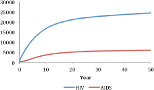
(b)

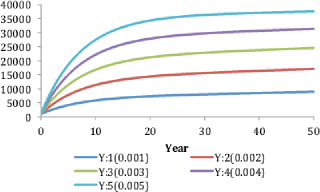
(c)

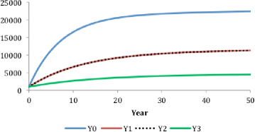
Figure 11.1. (a) Number of HIV and AIDS (before therapy), (b) Number of HIV infected (before therapy), (c) Number of HIV (after therapy)

(a)

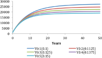
(b)

(c)

Figure 11.2. (a) Sensitivity of $d_{0}$ on $Y_{0}$, (b) Sensitivity of $d_{1}$ and $d_{2}$ on $Y_{1}$ and $Y_{2}$, (c) Sensitivity of $d_{3}$ on $Y_{3}$.

(a)

(b)

(c)

Figure 11.3. (a) Sensitivity of $d_{0}$ on $D_{z0}$, (b) Sensitivity of $d_{1}$ and $d_{2}$ on $D_{z1}$ and $D_{z2}$, (c) Sensitivity of $d_{3}$ on $D_{z3}$.

(a)

(b)

(c)

Figure 11.4. (a) Sensitivity of $\gamma_{0}$ on $D_{z0}$, (b) Sensitivity of $\gamma_{1}$ and $\gamma_{2}$ on $D_{z1}$ and $D_{z2}$, (c) Sensitivity of $\gamma_{3}$ on $D_{z3}$.

(a)

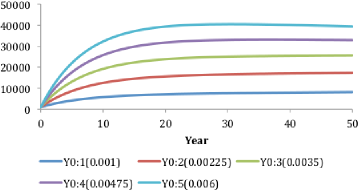
(b)

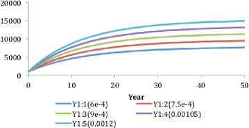
(c)

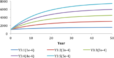
Figure 11.5. (a) Sensitivity of $\lambda_{0}$ on $D_{z0}$, (b) Sensitivity of $\lambda_{1}$ and $\lambda_{2}$ on $D_{z1}$ and $D_{z2}$, (c) Sensitivity of $\lambda_{3}$ on $D_{z3}$.

References

[1]Aalen, O.O., Farewell, V.T., De Angelis, D., Day, N.E.,
Gill, O.N. New Therapy explains the fall in AIDS incidence with a
substantial rise in number of persons on treatment expected. AIDS.
13 (1): 103-108. (1999).
[2]Anderson, R.M. The epidemiology of HIV infection:
variable incubation plus infectious periods and heterogeneity in sexual
activity. J. Roy. Statist. Soc. Ser. A 151, no. 1, 66–98 (1988)
[3]Anderson, R.M., May, R.M. Infectious diseases of humans.
Dynamics and Control. Oxford University Press. (1991)
[4]Artzrouni, M.A. (1992) modeled time-varying density
function for the incubation period of AIDS. J. Math. Biol. 31 , no.
1, 73–99 (1992)
[5]Becker, N.G., Lewis, J.J.C., Li Z.F., et al. Age-specific
back-projection of HIV diagnosis data Statistics in Medicine, 22 (13):
2177-2190 (2003)
[6]Brookmeyer, R., Gail, M.H. AIDS Epidemiology A Quantitative
Approach. Oxford University Press. New York. (1994).
[7]Brookmeyer, R., Gail, M.H. A method for obtaining
short-term projections and lower bounds on the size of the AIDS epidemic
J. Am. Stat. Assoc. 83 (402): 301-308 (1988).
[8]Castillo-Chavez, C., Cooke, K., Huang, W., Levin,
S. A. On the role of long incubation periods in the dynamics of acquired
immunodeficiency syndrome (AIDS). I. Single population models. J.
Math. Biol. 27, no. 4, 373–398 (1989).
[9]Conti, S., Masocco, M., Pezzotti, P., et al. Differential
Impact of Combined Antiretroviral Therapy on the Survival of Italian
Patients With Specific AIDS-Defining Illnesses. J. Acquir. Immu. Defici.
Synd. 25(5):451-458 (2000).
[10]Griffiths J, Lowrie D, Williams J An age-structured
model for the AIDS epidemic European J of Operational Research, 2000,
124 (1): 1-14.
[11]Hung, C.C, Chen, M.Y, Hsiao, C.F, Hsieh, S.M.,
Sheng, W.H., Chang, S.C. Improved outcomes of HIV-1-infected adults
with tuberculosis in the era of highly active antiretroviral therapy.
AIDS. 17(18):2615-2622 (2003)
[12]Kakehashi, M. A mathematical analysis of the spread
of HIV/AIDS in Japan IMA J math. appl. med. 15 (4): 299-311 (1998)
[13]May, R.M., Anderson, R.M., McLean, A.R. Possible demographic
consequences of HIV/AIDS epidemics. I. Assuming HIV infection always
leads to AIDS. Math. Biosci. 90, no. 1-2, 475–505 (1988)
[14]Nowak M.A., May R.M. Virus Dynamics, Oxford University
Press (2000)
[15]Perelson, A.S., Nelson, P.W. Mathematical analysis
of HIV-1 dynamics in vivo. SIAM Rev. 41, 1: 3-44 (1999)
[16]Rao, A.S.R.S., Kakehashi, M. A Combination of
Differential equations and Convolution in understanding the spread
of an epidemic. Sadhana - Proc. Ind. Acad. Sc, Engg, 29, 3: 305-313
(2004)
[17]Rao, A.S.R.S., Kakehashi, M. Incubation time
distribution in back-calculation applied to HIV/AIDS data in India.
Math. Biosci. Engg. no. 2, 263 - 277 (2005)
[18]Rao, A.S.R.S., Basu, S., Basu, A., Ghosh,
J.K. Parametric models for incubation distribution in presence of
left and right censoring. Indian Journal of Pure & Applied Mathematics
36(7):pp. 371-384 (2005)
[19]Rao, Arni S. R. Srinivasa; Thomas, Kurien; Sudhakar,
Kurapati; Maini, Philip K. HIV/AIDS epidemic in India and predicting
the impact of the national response: mathematical modeling and analysis.
Math. Biosci. Eng. 6 (2009), no. 4, 779–813,
[20]Castillo-Chavez C (1989). Mathematical and statistical
approaches to AIDS epidemiology. Edited by C. Castillo-Chavez. Lecture
Notes in Biomathematics, 83. Springer-Verlag, Berlin, (1989)
[21]Mouton, Y, Alfandari, S, Valette, M et al. Impact
of protease inhibitors on AIDS-defining events and hospitalizations
in 10 French AIDS reference centres. AIDS. 11(12):F101-F105 (1997)
[22]Wei, X.P., Ghosh, S.K., Taylor, M.E., et al. Viral
dynamics in human-immunodeficiency-virus type-1 infection Nature 373:
117-122. (1995)
[23]M. Over, E. Marseille, K. Sudhakar, J. Gold, I.
Gupta, A. Indrayan,S.K. Hira, N. Nagelkerke, A.S.R.S. Rao, P. Heywood.
Antiretroviral therapy and HIV prevention in India: Modeling costs
and consequences of policy options. Sex Transm Dis. 2006;33 (10 Suppl):S145-52.
[24]Gray R, Ssempiija V, Shelton J, Serwadda D, Nalugoda
F, Kagaayi J, Kigozi G, Wawer MJ. The contribution of HIV-discordant
relationships to new HIV infections in Rakai, Uganda. AIDS. 2011 Feb
14.
[25]Shafer LA, Nsubuga RN, White R, Mayanja BN, Chapman
R, O’brien K, Van der Paal L, Grosskurth H, Maher D. Antiretroviral
therapy and sexual behavior in Uganda: a cohort study. AIDS. 2011
Mar 13;25(5):671-8.
[26]Reynolds SJ, Makumbi F, Nakigozi G, Kagaayi J,
Gray RH, Wawer M, Quinn TC, Serwadda D. HIV-1 transmission among HIV-1
discordant couples before and after the introduction of antiretroviral
therapy. AIDS. 2011 Feb 20;25(4):473-7.
[27]Thirumurthy H, Jafri A, Srinivas G, Arumugam V,
Saravanan RM, Angappan SK, Ponnusamy M, Raghavan S, Merson M, Kallolikar
S. Two-year impacts on employment and income among adults receiving
antiretroviral therapy in Tamil Nadu, India: a cohort study. AIDS.
2011 Jan 14;25(2):239-46.
[28]Mahy M, Stover J, Stanecki K, Stoneburner R, Tassie
JM. Estimating the impact of antiretroviral therapy: regional and
global estimates of life-years gained among adults. Sex Transm Infect.
2010 Dec;86 Suppl 2:ii67-71.
[29]Pretorius C, Stover J, Bollinger L, Bacaï¿œr
N, Williams B. Evaluating the cost-effectiveness of pre-exposure prophylaxis
(PrEP) and its impact on HIV-1 transmission in South Africa. PLoS
One. 2010 Nov 5;5(11):e13646.
[30]Weber J, Tatoud R, Fidler S. Postexposure prophylaxis,
preexposure prophylaxis or universal test and treat: the strategic
use of antiretroviral drugs to prevent HIV acquisition and transmission.
AIDS. 2010 Oct;24 Suppl 4:S27-39.
[31]Eng B, Cain KP, Nong K, Chhum V, Sin E, Roeun S, Kim
S, Keo S, Heller TA, Varma JK. Impact of a public antiretroviral program
on TB/HIV mortality: Banteay Meanchey, Cambodia. Southeast Asian J
Trop Med Public Health. 2009 Jan;40(1):89-92.
[32]Rajagopalan N, Suchitra JB, Shet A, Khan ZK, Martin-Garcia
J, Nonnemacher MR, Jacobson JM, Wigdahl B. Mortality among HIV-Infected
Patients in Resource Limited Settings: A Case Controlled Analysis
of Inpatients at a Community Care Center. Am J Infect Dis. 2009;5(3):219-224.
[33]Salomon JA, Hogan DR. Evaluating the impact of antiretroviral
therapy on HIV transmission. AIDS. 2008 Jul;22 Suppl 1:S149-59.
[34]Johnson JA, Li JF, Wei X, Lipscomb J, Irlbeck
D, Craig C, Smith A, Bennett DE, Monsour M, Sandstrom P, Lanier ER,
Heneine W. 219. Minority HIV-1 drug resistance mutations are present
in antiretroviral treatment-naï¿œve populations and associate with reduced
treatment efficacy. PLoS Med. 2008 Jul 29;5(7):e158.
[35]Hallett TB, Gregson S, Dube S, Garnett GP. The impact
of monitoring HIV patients prior to treatment in resource-poor settings:
insights from mathematical modelling.PLoS Med. 2008 Mar 11;5(3):e53.
[36]Larson BA, Fox MP, Rosen S, Bii M, Sigei C, Shaffer
D, Sawe F, Wasunna M, Simon JL. 251. Early effects of antiretroviral
therapy on work performance: preliminary results from a cohort study
of Kenyan agricultural workers. AIDS. 2008 Jan 30;22(3):421-5.
[37]United Nations (2006). Department of Economic and
Social Affairs, Population Division (2006). World Population Prospects:
The 2007 Revision.
[38]Stover J, Walker N, Grassly NC, Marston M. Projecting
the demographic impact of AIDS and the number of people in need of
treatment: updates to the Spectrum projection package. Sex Transm
Infect. 2006 Jun;82 Suppl 3:iii45-50.
[39]Boyle B.A., Elion R., Cohen C.J., DeJesus E., Hawkins
T., Moyle G.J. Advances in HIV therapeutics: news from the 4th International
AIDS Society Conference. AIDS Read. 2007 Oct;17(10):484-90.
[40]Simcock M, Blasko M, Karrer U, et al. Treatment and
prognosis of AIDS-related lymphoma in the era of highly active antiretroviral
therapy: findings from the Swiss HIV Cohort Study. Antivir Ther. 2007;12(6):931-9.
[41]Mugavero MJ, Pence BW, Whetten K, Leserman J, Swartz
M, Stangl D, Thielman NM. Predictors of AIDS-related morbidity and
mortality in a southern U.S. Cohort. AIDS Patient Care STDS. 2007
Sep;21(9):681-90.
[42]Artzrouni M. Back-calculation and projection of the
HIV/AIDS epidemic among homosexual/ bisexual men in three European
countries: evalution of past projections and updates allowing for
treatment effects. Eur J Epidemiol. 2004;19(2):171-9.
[43]Golub JE, Saraceni V, Cavalcante SC, Pacheco AG,
Moulton LH, King BS, Efron A, Moore RD, Chaisson RE, Durovni B.The
impact of antiretroviral therapy and isoniazid preventive therapy
on tuberculosis incidence in HIV-infected patients in Rio de Janeiro,
Brazil. AIDS. 2007 Jul 11;21(11):1441-8.
[44]Rong, Libin; Feng, Zhilan; Perelson, Alan S. Emergence
of HIV-1 drug resistance during antiretroviral treatment. Bull. Math.
Biol. 69 (2007), no. 6, 2027—2060
[45]Rong, Libin; Feng, Zhilan; Perelson, Alan S. Mathematical
analysis of age-structured HIV-1 dynamics with combination antiretroviral
therapy. SIAM J. Appl. Math. 67 (2007), no. 3, 731—756.
[46]Cohen MS, Chen YQ, McCauley M et al. Prevention
of HIV-1 Infection with Early Antiretroviral Therapy.N Engl J Med.
2011 Jul 18. [Epub ahead of print]
[47]Joglekar, N.; Paranjape, R.; Jain, R.; et al.
(2011). Barriers to ART adherence & follow ups among patients attending
ART centres in Maharashtra, India, Indian Journal of Medical Research
Volume: 134 Issue: 6 Pages: 954-959.
[48]Rao, Arni S.R. Srinivasa and Hira S.K. (2003).
Evidence of Shorter Incubation period of HIV-1 in Mumbai , India.
International Journal of STD & AIDS, 14: 499-503.
[49]Rao, Arni S. R. Srinivasa, Thomas, Kurien;
Kurapati, Sudhakar; Bhat, Ramesh Improvement in survival of people
living with HIV/AIDs and requirement for 1st- and 2nd-line ART in
India: A mathematical model. Notices Amer. Math. Soc. 59 (2012), no.
4, 560–562.
[50]Boerma JT et al (2006). Monitoring the scale-up
of antiretroviral therapy programmes: methods to estimate coverage.
Bulletin of The WHO, 84, 2, 145-150.
[51]Srikantiah, P; Ghidinelli, M; Bachani, D; et
al. (2010). Scale-up of national antiretroviral therapy programs:
progress and challenges in the Asia Pacific region. AIDS Volume: 24
Supplement: 3 Pages: S62-S71.
[52]Monitoring of Antiretroviral Therapy in Resource
–limited settings: Discussion (http://www.medscape.com/viewarticle/726673_4)
(Browsed on 6 July, 2011)
[53]WHO (2010). Antiretroviral therapy for HIV infection
in adults and adolescents: recommendations for a public health approach.
– 2010 rev, World Health Organization.