The synchronization of stochastic oscillators

Abstract

We examine microscopic mechanisms for coupling stochastic oscillators so that they display similar and correlated temporal variations. Unlike oscillatory motion in deterministic dynamical systems, complete synchronization of stochastic oscillators does not occur, but appropriately defined oscillator phase variables coincide. This is illustrated in model chemical systems and genetic networks that produce oscillations in the dynamical variables, and we show that suitable coupling of different networks can result in their phase synchronization.

The concerted behaviour of different stochastic processes can be of considerable importance in a variety of situations. Examples from a biological context glass range from the synchronized firing of groups of neurons neuron to the occurence of circadian or ultradian cycles church ; tu in groups of metabolic and cellular regulatory processes, each of which is individually stochastic. Similar phenomena also occur in other areas of study, such as weather modeling or the study of coupled populations lloyd . It is therefore a moot question whether there is a sense in which two or more independent (or unrelated) stochastic phenomena can become temporally synchronized. In this Letter we consider mechanisms through which such synchronization can be effected, and examine measures through which the synchronization can be detected.

The synchronization of coupled nonlinear oscillators has been studied extensively in the past two decades. Both chaotic and nonchaotic oscillator systems can show complete synchronization, when all variables of the systems coincide, as well as more general forms such as phase, generalized, or lag synchronization kurths . Studies have examined a variety of different coupling schemes and topologies, and the robustness of synchronization to noise. In the typical cases examined, the noise is external and thus appears largely as additional stochastic terms in otherwise deterministic dynamical equations a ; hanggi .

For the systems we study here the evolution is intrinsically stochastic. Such systems do not follow deterministic equations of motion: a master equation describes the evolution of configurational probabilities master ,

$$\frac{d}{dt}P({\cal{C}},t)=-\sum_{{\cal{C^{\prime}}}}P({\cal{C}},t)W_{{\cal{C}}\to{\cal{C^{\prime}}}}+\sum_{{\cal{C^{\prime}}}}P({\cal{C^{\prime}}},t)W_{{\cal{C^{\prime}}}\to{\cal{C}}}$$ (1)

where in standard notation osw , $P({\cal{C}},t)$ is the probability of configuration ${\cal{C}}$ and the $W$’s are transition probabilities. The configurations that are realized as a function of time give a probabilistic description of the system as it traverses the state space of the problem.

Consider now two such independent systems, each of which can be described by a (reduced) master equation of the above form. Starting with similar configurations, ${\cal{C}}$, the subsequent evolution of each of the subsystems will typically be quite distinct. The concern here is to (a) examine conditions under which the two subsystems synchronize, namely follow very similar paths in the state space, and to (b) detect this phenomenon.

Our main result can be stated in general terms as follows. When the two systems are coupled by employing a mediating process, then variables of the two subsystems phase–synchronize, namely they vary in unison. Such synchronization depends on the nature and strength of the coupling and can persist even when fluctuations are large.

It is simplest to illustrate this through an example. The stochastic dynamics of the Brusselator model, which has been studied extensively brussel derives from consideration of the following “chemical” reactions gillespie

$$A_{1} \xrightarrow{c_{1}} X$$ (2)

$$A_{2}+X \xrightarrow{c_{2}} Y+A_{3}$$ (3)

$$2X+Y \xrightarrow{2c_{3}} 3X$$ (4)

$$X \xrightarrow{c_{4}} A_{4}.$$ (5)

A master equation formalism is exact for this system in the gas phase and in thermal equilibrium megillespie , and indeed is necessary when the number of molecules is small. On the other hand, in the thermodynamic limit, when fluctuations are negligible, one can derive a set of deterministic reaction–rate equations for the concentrations of species $X$ and $Y$,

$$\dot{x} = c_{1}-c_{2}x+c_{3}x^{2}y-c_{4}x\equiv f_{x}(x,y)$$ (6)

$$\dot{y} = c_{2}x-c_{3}x^{2}y\equiv f_{y}(x,y).$$ (7)

These rate equations usually have to be integrated numerically to determine the orbits (for the parameters here, a limit cycle). Similarly, the corresponding master equation cannot be solved analytically and recourse must be made to Monte Carlo simulations gillespie . The number of molecules of species $X$ or $Y$ (taking the volume to be unity) will vary in a stochastic manner, giving a (noisy) limit–cycle solution to Eqs. (2-5).

Another Brusselator system (denoted by similar equations, but with primed variables and parameters, say) would also naturally give a noisy limit cycle solution, the characteristics of which would depend on the parameters of the problem. Thus if the parameters $\{c_{i}\}$ and $\{c^{\prime}_{i}\}$ are different the evolution of the two subsystems will be independent and uncorrelated.

We consider two scenarios where the subsystems are coupled at the microscopic level. In the “direct” case, we take the species $X$ and $X^{\prime}$ to be identical: the subsystems share a common drive. We find that for any finite volume this coupling results in the temporal variation of species $Y$ and $Y^{\prime}$ rapidly becoming highly correlated, even if the fluctuations are large.

Alternately one may consider an “exchange” process, when species $X$ and $X^{\prime}$ can interconvert. This introduces an additional reaction,

$$X\xrightleftharpoons[c^{\prime}]{c}X^{\prime}$$ (8)

that serves to couple the subsystems, and depending on the rate of interconversion (governed by $c$ and ${c^{\prime}}$), species $Y$ and $Y^{\prime}$ show synchronization.

Although both direct as well as exchange coupling mechanisms effect synchronization, they differ in the details of how they act. Fig. 1 shows the variation of species $Y$ and $Y^{\prime}$ as a function of time, from stochastic simulations as well as the so–called chemical Langevin approach lange , which effectively adds stochastic noise to the deterministic dynamics, Eqs. (6-7). Clearly the two concentrations vary in unison. However, due to intrinsic stochastic fluctuations the two solutions do not become identical but only phase–synchronize rpk as we now show.

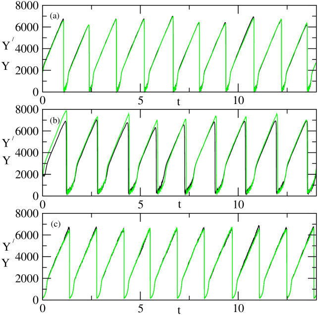
Figure 1: (Colour online) Species $Y$ and $Y^{\prime}$ as a function of time for the coupled Brusselator system. The parameter $c_{2}=50$ differs from $c^{\prime}_{2}=c_{2}+5$. The other parameters are $c_{1}=c^{\prime}_{1}=5000$, $c_{3}=c^{\prime}_{3}=0.000025$ and $c_{4}=c^{\prime}_{4}=5$. (a) Stochastic simulation results for $Y$ and $Y^{\prime}$ using direct coupling. (b) As in (a), but for the case of exchange coupling, Eq. (8) with $c=c^{\prime}=0.6$. (c) Results obtained by solving the chemical Langevin equation lange with $\gamma=0.01$.

To judge the phase synchronization of two stochastic oscillators, it is necessary to first obtain the phase for a single oscillator. The Hilbert phase of a signal $s(t)$ is obtained rpk by first computing its Hilbert transform,

$$\pi\bar{s}(t)=\mbox{P. V.~{}}\int_{-\infty}^{\infty}\frac{s(\tau)}{t-\tau}d\tau$$ (9)

(P. V. denotes principal value) and defining the instantaneous amplitude $A(t)$ and phase $\phi(t)$ through

$$A(t)e^{i\phi(t)}=s(t)+i\bar{s}(t).$$ (10)

The difference in the Hilbert phases $\phi$ and $\phi^{\prime}$ of the two stochastic oscillators is shown in Fig. 2. When the subsystems are uncoupled, the phase difference $|\phi-\phi^{\prime}|$ increases linearly in time on average since the oscillators evolve independent of one another. With coupling the two oscillators phase–synchronize and the phase difference fluctuates around a constant value.

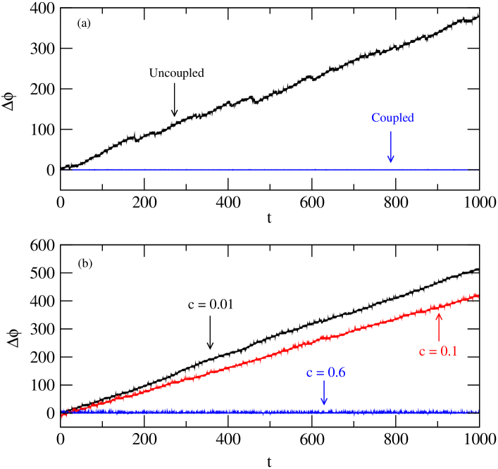
Figure 2: (Colour online) Phase difference with parameter mismatch for the Brusselator model for (a) direct coupling of species $X$ and $X^{\prime}$, and (b) exchange coupling, for different strengths.

The coupling schemes discussed here can bring about stochastic synchronization in a very general setting. Consider, for example, a model circadian oscillator that has been quantitatively studied in some detail recently genosc . Shown in Fig. 3 is the biochemical network for two such oscillators coupled with a common drive, namely two genetic circuits with a common activator. In effect a single activator binds to two promoter sites for repressor proteins $R$ and $S$, a fairly commonplace situation. Each individual circuit gives stochastic oscillations in the number of repressor molecules. When the two systems are coupled the stochastic oscillations of the two subsystems rapidly phase–synchronize. The synchronization is robust to parameter variation: in the examples shown in Fig. 4, the corresponding parameters of the two subsystems differ by as much as 10%; nevertheless the variables of the two systems oscillate in phase in a stable and sustained manner.

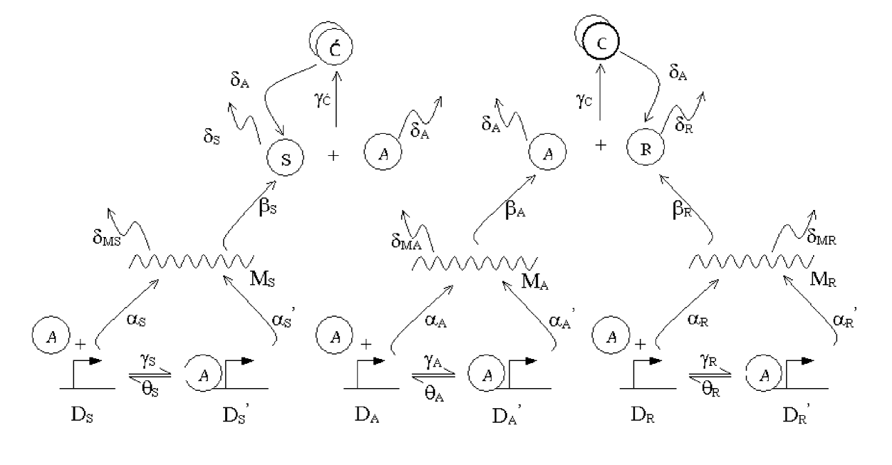
Figure 3: Biochemical network of the extended circadian oscillator model. $D_{A}$ and $D_{A}^{\prime}$ denote the number of activator genes with and without $A$ bound to its promoter respectively, and $D_{R}$, $D_{R}^{\prime}$ and $D_{S}$, $D_{S}^{\prime}$, refer to the two repressors driven by the common promoter $A$. $M_{A}$, $M_{R}$ and $M_{S}$ denote mRNA corresponding to the activator $A$, and the repressors $R$ and $S$. $C$ and $C^{\prime}$ corresponds to the inactivated complexes formed by $A$ and $R$, and $A$ and $S$ respectively. The constants $\alpha$ and $\alpha^{\prime}$ denote the basal and activated rates of transcription, $\beta$ the rates of translation, $\delta$ the rates of spontaneous degradation, $\gamma$ the rates of binding of $A$ to other components, and $\theta$ denotes the rates of unbinding of $A$ from those components. See param .

The temporal behaviour of the two repressors and their phase difference for both direct and exchange coupling are shown in Fig. 4. In (a) the two systems are initially uncoupled and therefore evolve independently. The coupling is switched on for $t\geq 2000$, leading rapidly to a constant phase difference, indicative of the phase synchronization (Fig. 4(b)). In the case of exchange coupling the genetic circuit differs somewhat from Fig. 3: the circuit of Ref. genosc is essentially doubled, and there is an additional activator $A^{\prime}$. Through the equivalent of Eq. (8) the activators of the two circuits are allowed to interconvert, and the two subsystems synchronize as can be seen in Fig. 4(c-d).

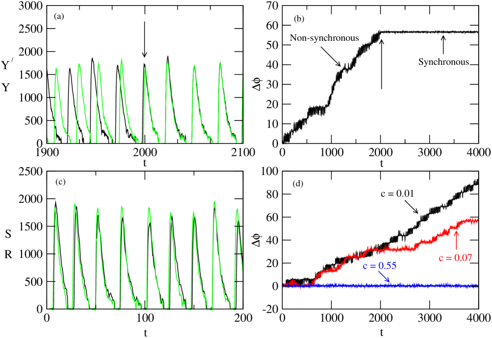
Figure 4: (Colour online) Temporal behaviour and phase difference of the repressors in the circadian oscillator model. (a) The repressors are initially uncoupled and the coupling is switched on (vertical arrow) at time $t\geq 2000$. (b) The corresponding phase difference, which becomes constant for $t\geq 2000$. (c) Time-series of the repressors oscillating in unison for diffusive coupling with $c=c^{\prime}=0.55$. (d) Phase differences for various $c$.

Examination of the macroscopic dynamics offers some clues as to how the stochastic oscillators synchronize. While the master equation description is formally exact at the microscopic level, the kinetic equations that describe the system at a macroscopic level can be derived from Eq. (1) by first obtaining the generating function representation, followed by a cumulant expansion nicolis to give a set of ordinary differential equations,

$$\dot{\bf{x}}={\bf{f}}({\bf{x}},t)+O(\frac{1}{V})+O(\frac{1}{V^{2}})+\ldots$$ (11)

in the variables $x_{i}={\langle X_{i}\rangle}/{V}$, namely the average concentrations, with “noise” corrections that depend on the system volume $V$. Coupling two such systems as discussed above would give a set of coupled stochastic differential equations, and the circumstances under which these will phase synchronize have been studied to some extent kurths ; neiman . The direct coupling, in the deterministic limit gillespie ; cle leads to dynamical equations which are similar (but not identical) to those that derive from the coupling scheme proposed by Pecora and Carroll pecora for the synchronization of chaotic oscillators. Although it is not possible to define Lyapunov exponents for stochastic systems, analysis of the deterministic limit gives indications of what coupling schemes could be effective. Making species $Y$ the common drive between the two Brusselator subsystems does not serve to synchronize them but instead leads to the stochastic analogue of oscillator death.

Similarly, the exchange process, Eq. (8) results in diffusive coupling boccaletti in the kinetic equations for the species $X$ and $X^{\prime}$, namely terms of the form $c(x^{\prime}-x)$. The conditions under which this form of the coupling leads to synchronization have also been studied boccaletti . As can be seen from the examples presented here, the systems synchronize when the effective coupling exceeds a threshold strength (Figs. 2(b) and 4(d)). The rate of growth of the phase difference vanishes at this threshold as a power wang .

Stochastic oscillators appear to effectively synchronize independent of the size of fluctuations, in a manner similar to chaotic synchronization pecora . However, even when the parameters are identical, exact synchronization is not possible and the systems can only phase–synchronize.

The synchronization of stochastic oscillators thus has similarities to the analogous process in deterministic dynamical systems (both with and without added noise), but also important differences. The mechanisms that we have described here pertain to systems with intrinsic stochasticity, and are therefore in a nonperturbative limit.

The coupling schemes that we have proposed here can find application in the design and control of synthetic biological networks where synchronous oscillation may be a desirable feature. McMillen et al. kopell have shown that intercell signaling via a diffusing molecule can couple genetic oscillators and effect synchrony. The present results indicate that such phase synchrony can emerge under very general conditions with high levels of ambient noise. In a related vein, one can speculate that similar mechanisms underlie the synchrony that is so dramatically evident in cellular processes. As recent time–resolved microarray experiments of yeast have revealed, the multitude of variable gene expression patterns classify into a small number of groups, all genes of a given group having very similar temporal variation profiles tu . We have observed that the above coupling schemes are effective in synchronizing ensembles of stochastic oscillators nandi . Other physical situations where such mechanisms may be relevant are in the study of coupled ecosystems or coupled weather systems: individual subsystems show stochastic dynamics, which however have phase synchrony lloyd .

Although we have discussed the explicit case of stochastic oscillators, there is reason to believe that similar microscopic intersystem couplings can bring about temporal correlations in more general stochastic systems. Investigations of such phenomena are currently under way nandi .

This research is supported by grants from the DBT, India (to RR) and the CSIR, India through the award of Senior Research Fellowships (to AN and SG) and a Research Associateship (to RKBS). We thank M Bennett, T Gross, and J K Bhattacharjee for helpful correspondence.

References

- (1) L. Glass, Nature 410, 277 (2001).
- (2) A. Neiman et al., Phys. Rev. Lett. 82, 660 (1999).
- (3) B. P. Tu, A. Kudlicki, M. Rowicka and S. L. McKnight, Science, 310, 1152 (2005).
- (4) See e. g. S. Tavazoie, J. D. Hughes, M. J. Campbell, R. J. Cho and G. M. Church, Nature Genetics 22, 281 (1999).
- (5) A. L. Lloyd and R. M. May, Trends Ecol. Evol. 14, 417 (1999).
- (6) A. Pikovsky, M. Rosenblum and J. Kurths, Synchronization: A universal concept in nonlinear science, (Cambridge University Press, Cambridge, 2001).
- (7) V. S. Afraimovich, N. N. Verichev, and M. I. Rabinovich, Radiophysics and Quantum Electronics, 29, 795 (1986).
- (8) J. A. Freund, L. S. Geier and P. Hänggi, Chaos 13, 225 (2003).
- (9) D. A. McQuarrie, J. Appl. Prob. 4, 414 (1967).
- (10) I. Oppenheim, K. E. Shuler and G. H. Weiss, Stochastic Processes in Chemical Physics: The Master Equation, (The MIT Press, 1977).
- (11) I. Prigogine and R. Lefever, J. Chem. Phys. 48, 1695 (1968); J. J. Tyson, J. Chem. Phys. 58, 3919 (1973).
- (12) D. T. Gillespie, J. Phys. Chem. 81, 2340 (1977).
- (13) D. T. Gillespie, Physica A 188, 404 (1992).
- (14) D. T. Gillespie, J. Chem. Phys. 113, 297 (2000); C. W. Gardiner, Handbook of Stochastic Processes, (Springer-Verlag, Berlin, 1985).
- (15) L. M. Pecora and T. L. Carroll, Phys. Rev. Lett. 64, 821 (1990).
- (16) In practice, at the end of each integration step, a term is added to the solution of the deterministic equations of motion, being the strength of the Gaussian noise cle .
- (17) M. G. Rosenblum, A. S. Pikovsky, and J. Kurths, Phys. Rev. Lett. 76, 1804 (1996).
- (18) M. G. Vilar, H. Y. Kueh, N. Barkai and S. Leibler, Proc. Natl. Acad. Sci. (USA) 99, 5988 (2002).
- (19) G. Nicolis and I. Prigogine, Self-Organization in Nonequilibrium Systems (Wiley, New York, 1977).
- (20) We take the following values for the reaction rates genosc : , , , , , , , , , , , , , , , , , , , . The initial conditions are , . The cell has a single copy of the activator and repressor genes: , and the volume is assumed to be unity.
- (21) S. Boccaletti, J. Kurths, G. Osipov, D. L. Valladares and C. S. Zhou, Phys. Rep. 366, 1 (2002).
- (22) M. Wang, Z. Hou, H. Xin, J. Phys. A 38, 145 (2005).
- (23) A. Neiman, Phys. Rev. E 49, 3484 (1994).
- (24) D. McMillen, N. Kopell, J. Hasty and J. J. Collins, Proc. Natl. Acad. Sci. (USA) 99, 679 (2002).
- (25) A. Nandi, Ph.D Thesis, JNU, 2007.