Learning with incomplete information
- and the mathematical structure behind it -

Learning and the ability to learn are important factors in development and evolutionary processes [1]. Depending on the level, the complexity of learning can strongly vary. While associative learning can explain simple learning behaviour [1, 2] much more sophisticated strategies seem to be involved in complex learning tasks. This is particularly evident in machine learning theory[3] (reinforcement learning [4], statistical learning [5]), but it equally shows up in trying to model natural learning behaviour [2]. A general setting for modelling learning processes in which statistical aspects are relevant is provided by the neural network (NN) paradigm. This is in particular of interest for natural, learning by experience situations. NN learning models can incorporate elementary learning mechanisms based on neuro-physiological analogies, such as the Hebb rule, and lead to quantitative results concerning the dynamics of the learning process [6]. The Hebb rule, however, cannot be directly applied in all cases, and in particular for realistic problems, such as “delayed reinforcement” [4, 6], the sophistication of the algorithms rapidly increases. We want to present here a model which can cope with such non trivial tasks, while still being elementary and based only on procedures which one may think of as natural, without any appeal to higher strategies [7]. We can show the capability of this model to provide good learning in many, very different settings [7, 8, 9]. It may help therefore understanding some basic features of learning.

Any realistic form of learning is in some sense learning from experience, since a learner interacts with an “environment”, appraises this interaction and consequently changes its “internal structure” according to some criteria. In models of biological behaviour, as well as in the design of information processing systems, the control for the appraisal procedure – food, pleasure, success, assessment of result – is formalized as some kind of reinforcement. Normal “experience” can, however, rarely be encoded into a reinforcement matrix relating actions with their results in a one-to-one manner, and a learner faces the additional task to interpret the environmental feedback before rewriting it as an update of its internal (cognitive) structure. An urgent problem, for example, with which an “agent”, either natural or artificial, may be confronted is to learn solely from the final success/failure of a series of consecutive actions, without direct information about the particular fitness of each of them, such as learning to coordinate its muscles in moving, learning a labyrinth or playing chess. Another case may be that of a feedback which only differentiate between the presence or absence of a certain kind of patterns in a mixture, such as sorting out unpalatable components in food, or realizing that some actions out of many were useful, without knowing which. Can sale statistics, for instance, reveal what exactly makes a good commercial?

How non-trivial such problems are can be seen from the sophisticated algorithms developed for so called “delayed reinforcement” in the framework of machine learning theories [4, 10]. In this perspective realistic, complex learning situations seem to require the availability of strategies and involved procedures before reinforcement can provide effective feedback mechanisms. In an evolutionary perspective of the development of learning capabilities, however, the question then arises as to how such strategies and procedures could have developed in the first place. If reinforcement were to be a general or even fundamental element involved in effecting behavioural change, one would expect reinforcement learning to act in particular at an intermediary level which is simple enough not to depend on involved strategies, yet sophisticated enough to allow complex behaviour to evolve.

Aside from such basic questions, it should be interesting in itself to develop some understanding of the capabilities of simple reinforcement learning procedures which do not depend on involved strategies to deal with cases of non-specific information.

A problem of non-specific reinforcement can be defined as follows: the reward is global, regards the cumulative result of a series of actions and the reinforcement acts non-specifically concerning these actions [11]. We ask whether there may exist elementary mechanisms to solve such problems, which may have developed also under natural conditions and which may hint at basic features of learning. For this we must not only demonstrate the existence of such mechanisms, but also uncover their structural features.

In previous papers [7], [8], [12] we introduced and studied a learning algorithm for neural networks (NN) which deals with this problem. The NN setting allows a systematic study by both numerical and analytic methods. It provides a framework to study learning with non-specific reinforcement which is transparent, and pertains to the basic machinery on which learning is believed to take place. NN thus can achieve complex information processing capabilities using mechanisms simple enough to have plausibly developed under natural conditions. Due to their general computational capabilities NN can model various levels of learning processes – biological, behavioural or cognitive [6].

The first step of our analysis begins by casting the problem into a classification task for a perceptron. In its simplest version, this is a network consisting of an array of $N$ input neurons projecting synapses onto a single output neuron. The active and inactive states of the neurons are encoded as $+1$ and $-1$ respectively. The “cognitive structure” of the network is encoded in the values $J_{i}$, $i=1,\dots,N$, of the synapse strengths, also called weights. The inputs to the network (the “patterns” which must be classified) are strings of $N$ binary values $\xi_{i}\in\{\pm 1\}$ loaded on the input layer. These values are weighted by the corresponding synapse strengths and transmitted to the output neuron, where they are added to define a “potential” which, according to its sign, triggers the output neuron to $s=\pm 1$ accordingly attributing the pattern ${\bm{\xi}}=(\xi_{i})$ to the class $s$.

The standard learning problem is stated by asking a “student” perceptron to implement a given classification rule. The rule is provided by a “teacher” perceptron with the same architecture, whose synapses $B_{i}$ are given and fixed. Student and teacher have access to the same inputs ${\bm{\xi}}$. We thus have

$$s={\rm sign\,}\left(\frac{1}{\sqrt{N}}\sum_{i=1}^{N}J_{i}\xi_{i}\right)\ ,\qquad t={\rm sign\,}\left(\frac{1}{\sqrt{N}}\sum_{i=1}^{N}B_{i}\xi_{i}\right)\ .$$ (1)

The student has access to the teacher’s output $t$ which provides the rule-based classification of the inputs, but not to the teacher’s rule represented by its weight vector ${\bm{B}}=(B_{i})$. The student learns from a stream of inputs classified by the teacher, ${\bm{\xi}^{\mu}}\to t^{\mu}$, $\mu=1,2,\dots$, adapting its own weights in response to these data in such a way as to reduce the number of cases where its own classification ${\bm{\xi}^{\mu}}\to s^{\mu}$ disagrees with that provided by the teacher.

A classical, and neuro-biologically motivated learning rule is the so-called Hebb rule, where synapses change in response to coincidence of pre- and post-synaptic activity. In the present setting the appropriate formulation of Hebb’s rule for the student performing the classification ${\bm{\xi}^{\mu}}\to s^{\mu}$ would take the form $\Delta J_{i}^{\mu}=J_{i}^{\mu+1}-J_{i}^{\mu}\propto s^{\mu}\xi_{i}^{\mu}.$

In order to turn this simple form of associative adaptation into learning, it must be supplemented with some form of feedback concerning the ‘quality’ of the associations. In learning rules traditionally used in studies of supervised learning within the student-teacher scenario the proportionality ‘constant’ in Hebb’s rule is made to depend on the difference between the teacher and student answers. The two most popular algorithms are the supervised Hebb (H) and Perceptron (P) learning algorithms, defined by

$$\Delta J_{i}^{\mu}=at^{\mu}\xi_{i}^{\mu}\qquad\mbox{(H)}\qquad\mbox{and}\qquad\Delta J_{i}^{\mu}=\frac{a}{2}|s^{\mu}-t^{\mu}|t^{\mu}\xi_{i}^{\mu}\qquad\mbox{(P)}\ ,$$ (2)

respectively. Written in this form both algorithms assume immediate and direct control over the student’s synapses, which in a way amounts to assuming that a teacher is able to clamp a desired output onto the student neuron (e.g., by providing an ‘evaluating’ stimulus through some other channel – see, e.g. [1]).

In standard “supervised on-line learning” the student is told after each instance what the right answer would have been (specific feedback). In our approach, however, according to our paradigm the student can only receive a non-specific reinforcement about some global degree of correctness of its answers over many instances. More precisely the student is presented with series (“bags”) of patterns and only obtains information concerning its cumulative performance for the bag as a whole, not with respect to each pattern in the bag. The non-trivial learning problem is to implement this global information into a local updating rule for the synapses.

The learning algorithm we propose can be described as consisting of two phases. To be specific, we assume that each bag $q$ contains the same number $L$ of patterns.

In the first phase the student processes the patterns in a bag $q$ one by one and modifies its synapses by simple, associative Hebbian learning, using its own classifications made on the basis of its momentary synapse values:

$${\rm I.\ :}\ \ J_{i}^{(q,l+1)}=J_{i}^{(q,l)}+\frac{a_{1}}{\sqrt{N}}s^{(q,l)}\xi_{i}^{(q,l)}\ ,\qquad l=1,\dots,L,$$ (3)

with $s^{(q,l)}={{\rm sign\,}}\left(\frac{1}{\sqrt{N}}\sum_{i=1}^{N}J_{i}^{(q,l)}\xi_{i}^{(q,l)}\right)$ being the student classification of pattern $(\xi_{i}^{(q,l)})$.

In the second phase the student obtains information about its global performance on a whole bag of patterns and corrects its synapses by “reconsidering” the steps of the first phase, and by partially undoing them in an indiscriminate way, to an extent that depends on the (likewise indiscriminate) global error over them, independently on which steps were in fact correct and which not. This phase can be seen as Hebbian “unlearning”:

$${\rm II.\ :}\ \ J_{i}^{(q+1,1)}=J_{i}^{(q,L+1)}-e_{q}~{}\frac{a_{2}}{\sqrt{N}}\sum_{l=1}^{L}\omega_{l}s^{(q,l)}\xi_{i}^{(q,l)},$$ (4)

where the on-line error $e_{q}$ is a measure of the disagreement to the teacher and defines the specific problem (see below). In (4), the $\omega_{l}$ can be 1 or 0 with probabilities $\rho$ and $1-\rho$, respectively, which accounts for the possibility that the replay during the second phase may be imperfect: the student may not recall all associations established during the first phase.

The procedure, so to say, is specific but blind association in the first phase, qualified but non-specific reinforcement in the second phase. We called this algorithm therefore Association-Reinforcement (AR) - Hebb algorithm.

It is interesting to note that a kind of replay as that involved in the Phase II of our algorithm apparently can be observed in rats on track running tasks [13]. This is considered to correspond to memory consolidation. Since experiences are usually not neutral, but also imply valuations, it is suggestive that in such replay not only neutral memories are consolidated, but memories evaluated by some measure of success (finding or not finding food at the end of the track, for instance). This would mean observing here a mechanism akin to the re-weighting replay of the Phase II of our learning model. Hebbian unlearning mechanisms via replay of data previously exposed to has been discussed also in other contexts [14]. Concerning Phase I this just represent strengthening of its own associations by repetition. Therefore the “AR-Hebb” algorithm not only appears natural behaviourally, but it may also have a neuro-physiological basis.

It turns out that only the ratio $\lambda=a_{1}/a_{2}$ of learning-rates in phase I and II is relevant for the analysis. Hence we shall work mostly with $a_{2}=1$, hence $\lambda=a_{1}$. It measures the strength of the local “associative” compared to the global “corrective” step.

For a perceptron, the progress of learning depends on the evolution of the angle between the student’s and the teacher’s weight vectors $\bm{J}$ and $\bm{B}$. At fixed $\bm{B}$, the relevant quantities are therefore the normalized scalar products $R=N^{-1}\bm{J}\cdot\bm{B}$ and $Q=N^{-1}\bm{J}\cdot\bm{J}$, commonly referred to as overlaps. Without loss of generality, one can assume the normalization $N^{-1}\bm{B}\cdot\bm{B}=1$. For unbiased inputs, the generalization error $\epsilon_{G}$, i.e., the probability of disagreement between student and teacher, can then be expressed in terms of $R$ and $Q$, $\epsilon_{G}=\frac{1}{\pi}\arccos(R/\sqrt{Q})$. The overlaps $R$ and $Q$ are also order parameters in the sense that the dynamics of learning can at a macroscopic level be fully described in terms of $R$ and $Q$ alone. The main elements of a derivation of this result are given in Elements of the analysis below.

Note that $Q$ controls the relative learning rate (the larger $Q$, the smaller the relative synaptic change induced by a single learning learning step).

For the case to be presented first, the non-specific reinforcement uses the average error of the student’s guesses for the whole bag (this is, up to a normalization, the cumulated, global error). For simplicity of reference we call this the “average error” (AE) problem – see eq. (8). At no moment does the student know whether his particular classifications are correct or or incorrect; he is only informed about the fraction of correct answers over the whole bag. The patterns are produced randomly.

The exciting result of this study is that stable perfect learning can be achieved in spite of the non-specific reinforcement! The most interesting feature is the dependence of learning on $\lambda$, the strength of the associative step as compared with the corrective one. It is found that the asymptotic decay of the generalization error $\epsilon_{G}$ as a function of the number $q$ of pattern-bags used for learning is described by a power-law, $\epsilon_{G}\sim q^{-p}$ with an exponent $p$ that depends on $\lambda$ — an unusual feature in neural network learning. But even more compelling is the appearance of a threshold $\lambda_{c}$ below which no learning is possible, whereas for $\lambda>\lambda_{c}$ perfect learning is always achieved. The exponent $p$ is a decreasing function of $\lambda$, so that learning becomes more efficient as $\lambda\searrow\lambda_{c}$. The value of $\lambda_{c}$ itself depends on $L$ and on the initial value $Q_{0}$ chosen for the order parameter $Q$, that is, on the initial learning rate ($1/\sqrt{Q_{0}}$). There is no such non-zero threshold for $L=1$, where $0\leq\lambda\leq\frac{1}{2}$ just interpolates between the supervised Hebb rule (H) at $\lambda=0$ and the Perceptron algorithm (P) at $\lambda=\frac{1}{2}$ in (2).

Figure 1: Numerical simulation of the AE problem: the learner is presented with bags of patterns, feedback is given only via the average (or total) error made over the whole bag. We plot the generalization error, $\epsilon_{G}$ vs the normalized number of patterns $\alpha=qL/N$. Each of the bags contains $L=10$ patterns; the size of the input layer is $N=100$. Initial conditions are random with $R(0)=0$ hence $\epsilon_{G}(0)=0.5$, and $Q(0)=10^{4}$. The replay phase is complete, i.e. $\rho=1$ (full circles, empty circles and crosses) or only partial ($\rho=0.5$, asterisks). For $\lambda=0.120$ (full circles) no generalization is observed, whereas for $\lambda=0.125$ (empty circles and asterisks) and $\lambda=0.250$ (crosses) perfect generalization is achievable. The lines represent the asymptotic behaviour expected from the analytic study $\epsilon_{G}(\alpha)\propto\alpha^{-\frac{1}{2L\lambda}}$.

Fig. 1 shows typical results of numerical simulations of the learning process with AE feedback for three values of $\lambda$. For the simulations the generalization error is measured by comparing the student and teacher answers on a random set of $10^{4}$ patterns.

Below $\lambda_{c}$ (which for the given initial conditions is located between $0.120$ and $0.125$) the generalization error initially decreases with increasing number $q$ of processed bags, then suddenly returns to a value very close to 0.5 and stays there ever after so that generalization is very poor in the long run. Just above $\lambda_{c}$, learning is rapid but may be disrupted by finite size fluctuations, which entail that the threshold $\lambda_{c}$ is somewhat fuzzy at finite $N$, becoming sharp only in the limit $N\to\infty$, in complete analogy to phase transitions in condensed matter systems. Further above $\lambda_{c}$ finite-size fluctuations cease to be effective in disrupting learning, but convergence to perfect generalization is also slower. The plot gives $\epsilon_{G}$ vs the normalized number of processed patterns $\alpha=qL/N$. The straight lines indicate the asymptotic behaviour expected for the corresponding $\lambda$ from the analytic theory.

Indeed, the results observed in the simulations can be derived analytically in the limit of large number $N$ of input-neurons (“thermodynamic limit”), in which the dynamics of the order parameters $R$ and $Q$ is shown to be governed by an autonomous set of coupled non-linear flow equations. See Elements of the analysis below.

This allows us to proceed to the second step, that of answering structural questions. The mathematical structure uncovered in this way shows that the global properties of the macroscopic learning dynamics are governed by a pair of fixed points, one fully stable, and the other partially stable with an attractive and a repulsive direction.

Figure 2: Analytic study of the AE problem, $L=10$. Shown are the generalization error $\epsilon_{G}$ vs $\alpha$ (left), and the flow of the learning dynamics in the $\epsilon_{G},\sqrt{Q}~{}-$plane (right) for fixed initial condition $R(0)=0$, $Q(0)=10^{4}$, and $\lambda=0.100$ (doubly dotted line), 0.138 (dotted), 0.139 (solid) and 0.250 (dashed line). The threshold appears at $\lambda_{c}\simeq 0.1385$, for which the initial condition is exactly on the attractive manifold of a partially stable fixed point. The attractive fixed point (A) and the partially stable fixed point (X) are clearly identifiable. The initial condition is marked with a $0$ in the plot. The straight lines on the left plot represent the asymptotic power laws with $p=\frac{1}{2L\lambda}$.

In Fig. 2 we present analytical results for the learning process as obtained by solving the flow equations (16), (17). The left panel is to be compared with the simulation results shown in Fig. 1. In the right panel, which shows the phase-flow of the learning dynamics in the $\epsilon_{G},\sqrt{Q}~{}-$plane, we can clearly discern the existence of a separatrix connecting the starting point and a partially stable fixed point with an attractive and a repulsive direction. The repulsive manifold directs the flow of the learning dynamics either towards large $Q$ and perfect generalization, or towards small $Q$ and an all-attractive fixed point of poor generalization. The alternative is decided by $\lambda$ which determines on which side of the separatrix the initial condition finds itself. By changing $\lambda$ as we do here, we actually move the fixed points around, and continuously deform the repulsive and the attractive manifolds, thereby sweeping the separatrix across the initial condition. Exactly at $\lambda_{c}$ the initial condition is found to lie on the separatrix. The structure indicated here fully explains the behaviour described above. The thresholds are crisp, of course, as there are no longer any finite size fluctuations. By comparing with results shown in Fig. 1 the finite-size correction of $\lambda_{c}$ at $N=100$ is found to be approximately 15%.

The mathematical structure lying behind our results suggests that they are stable against changing parameters and further details of the learning process, and in fact may hint at some general properties of our learning paradigm. A number of further studies were performed in order to substantiate this suggestion.

First, we investigated what happens if the “replay” in Phase II is not perfect — as a way to describe the possibility that the student may not ‘remember’ all instances encountered during Phase I. We modelled this by randomly including each instance of Phase I only with probability $\rho\leq 1$ in the unlearning step of Phase II. It turned out that all features observed for complete replay are preserved; for the asymptotic domain of good generalization the modification amounts to a re-scaling of the learning parameter $\lambda\to\lambda/\rho$ [7] – see Fig. 1.

Another possibility concerns randomly varying bag sizes $L$ used in learning. These, too, lead to results qualitatively unchanged when compared to the case of fixed $L$.

The next modification concerns the nature of the on-line error $e_{q}$ used in the reinforcement phase. We investigated a case where the student is only told the number of patterns of, say, class $+1$ in a bag, which he or she can compare with the number perceived to belong to that class by him/herself – see eq. (9). We called this the “hidden instance problem” (HI); it is a version of the so called “multiple instance problem”. The information received by the student thus has an increased degree of non-specificity (since, e.g., $e_{q}=0$ does not yet imply that the student has found the correct classification!). Nevertheless the performance of our learning model for this problem is very similar to that for the AE-problem. This can be seen both in simulations and in the corresponding analytic theory. The quantitative details are different, but the general behaviour is the same: Once more, we find a threshold $\lambda_{c}$, below which generalization remains poor in the long run, and a $\lambda$-dependent asymptotic power-law decay of the generalization error above the threshold [9].

A further extension looked into using structured input data in the classification task to be learnt, as a highly schematic way to model learning in a structured environment. Once more, similar results were obtained [8]. However, some supplementary tuning of the learning rate $\lambda$ was necessary, as indeed for the corresponding standard supervised algorithms dealing with the same problem. The dynamics itself is more complex, requiring three order parameters for a full macroscopic description instead of two. Yet again we observe that the parameter $\lambda$ must exceed a threshold $\lambda_{c}$, which depends on initial conditions, in order to achieve asymptotically perfect generalization.

Figure 3: Numerical simulation for a committee machine with $K=3$ hidden units and $N=100$ input units, AE problem with $L=5$: generalization error $\epsilon_{G}$ vs $\alpha$. Here $\lambda=0.260$ (full circles), 0.280 (circles) and 0.320 (crosses). The straight lines represent power-law fits to the asymptotic behaviour with exponents $p=0.16$ (solid line) and $p=0.085$ (dashed line), respectively.

In the cases discussed above we investigated single-layer networks, for which the solvable classification tasks are limited to the class of so-called “linearly separable” problems. This means that problems in a different complexity class, and presumably some of the more realistic ones, can at first sight not be solved by such networks, irrespectively of the learning algorithm used to train them, while they can be attacked by multi-layer networks.

It is now well known that the limits of linear separability can be transcended by the use of preprocessing and kernel methods [16], so as to provide the capability for universal classification while adhering to the perceptron as the trainable neural element.

Nevertheless, in order to lend further credibility to the hypothesis that non-specific reinforcement could provide a basic learning mechanism at work also beyond the single neuron level, and thereby plausibly contribute to the evolution of complex information processing capabilities in neural architectures, we investigate its performance on a simple multi-layer network [9], the so called “committee machine”. This is a two-layer network with the neurons of the second (hidden) layer – the committee – transmitting their state via fixed synapses to the output neuron. Only the synapses from the input neurons to committee members can be modified in the learning process.

There is an important second motivation, beyond that of demonstrating the viability of the non-specific reinforcement principle for training simple multi-layer networks, capable of performing classifications outside the linearly separable class: It is related to the fact that the single output of a multi-layer networks is itself non-specific in the sense of not revealing which of possibly several states of the hidden layer was responsible for it. Specifically, in the case of a committee-machine producing a simple majority vote of the committee members, no information is revealed as to which subset of the committee was backing the majority vote. This is non-specificity with respect to contributions of hidden nodes (for simplicity referred to as ‘non-specificity with respect to space’), whereas the AR - Hebb algorithm introduces an element of non-specificity with respect to time. By using the AR - Hebb algorithm to train a committee machine, we combine non-specificities in space and time, and the natural question arises whether this further reduction of the information used for feedback still permits that a rule — represented by a teacher committee of the same architecture — can be picked up on the basis of classified inputs alone.

We are able to report here recent results about this system. The version we have looked at is a “graded” version producing as its output the sum of the outputs of all committee members, without performing a final sign-operation on that sum. The simulations do indeed show convergence to perfect generalization, and a threshold in the learning parameter $\lambda$, as for the perceptron. See Fig. 3. However, this turns out to be combined with an even more complex picture of the evolution of the order parameters, hinting at a more complicated fixed point structure in the phase flow. E.g., a partially stable fixed point representing the student committee in a state where its hidden nodes have not yet specialized to represent one of the hidden nodes of the teacher committee exists [17] which interferes with the fixed point specifically associated with the unspecific delayed reinforcement. The interference between fixed points entails that effects of finite size fluctuations are stronger. The analytic study of the algorithm in terms of flow equations involves more order parameters (the mutual overlaps between weight vectors of all combinations of hidden nodes of student and teacher committee) and is is thus more difficult, but a number of special results strengthen the findings from the numerical simulations.

To summarize, a simple learning algorithm based on local Hebb-type synaptic modifications can solve various non-specific reinforcement problems. The algorithm seems applicable to a broad range of different situations, which hints at a high level of generality. It is interesting that such a simple algorithm can cope with complex learning problems, and this makes it a candidate for a basic mechanism in learning. As a model for biological developments it indicates that feedback non-specificity can be dealt with at the elementary neuronal level by mechanisms which are simple enough to have plausibly developed during the early stages of evolution. A very peculiar aspect is the essential role of both, local Hebb potentiation and global correction via replay.

Note that the correction in phase II of the algorithm respects an important information-theoretic symmetry: the synaptic correction in response to an indiscriminate feedback is indiscriminate in the same sense. Any deviation from this symmetry would entail that the learning mechanism creates a hypothesis about its environment for which the environmental feedback does not provide any evidence. This is in fact in fairly close analogy with Bernoulli’s principle of insufficient reason according to which the best assumption in an information-theoretic sense about a random variable of which we have no knowledge whatsoever apart from the range of values it can take, is to assume that its distribution is uniform over the range of possible values.

Some features of the learning behaviour described by this model may also show up in more complex non-specific feedback situations. In a behavioural setting, for instance, we find commitment to one’s own experiences and global, critical consideration of the results as necessary prerequisites for learning under the conditions of non-specific feedback. In the interaction between these two factors the randomness of experiences is shaped into a knowledge landscape. Nevertheless in our eyes the first merit of this model is to provide an elementary mechanism for learning from experiences with non-specific feedback which may be relevant in an evolutionary perspective.

Elements of the analysis

The synapse from the $i$-th input neuron ($i=1,\dots,N$) onto the output neuron is denoted $J_{i}$ for the student, $B_{i}$ for the teacher. The former change under learning, the latter are fixed (randomly given). The patterns in the bag $q$ are denoted $\xi_{i}^{(q,l)}$, $l=1,\dots,L$, they are random series of $\pm 1$’s. The output of the student and of the teacher for a given pattern are, respectively:

$$s^{(q,l)}={\rm sgn}\left(\frac{1}{\sqrt{N}}\sum_{i=1}^{N}J_{i}^{(q,l)}\xi_{i}^{(q,l)}\right),\quad t^{(q,l)}={\rm sgn}\left(\frac{1}{\sqrt{N}}\sum_{i=1}^{N}B_{i}\xi_{i}^{(q,l)}\right).$$ (5)

The teacher synapses are normalised to $\frac{1}{N}\sum_{i=1}^{N}B_{i}^{2}=1$. By rescaling the student synapses with $a_{2}$, $J_{i}^{(q,l)}/a_{2}\to J_{i}^{(q,l)}$, we remain with $\lambda=a_{1}/a_{2}$ as the only relevant learning parameter.

The two phases of the updating algorithm are then

$$J_{i}^{(q,l+1)} = J_{i}^{(q,l)}+\frac{\lambda}{\sqrt{N}}s^{(q,l)}\xi_{i}^{(q,l)}\ ,\qquad l=1,\dots,L$$ (6)

$$J_{i}^{(q+1,1)} = J_{i}^{(q,L+1)}-e_{q}\frac{1}{\sqrt{N}}~{}\sum_{l=1}^{L}\omega_{l}s^{(q,l)}\xi_{i}^{(q,l)}\ .$$ (7)

For the remainder of the present analysis we shall for simplicity restrict ourselves to the case where replay during phase II is complete, i.e., $\omega_{l}\equiv 1$.

We define the “average error” (AE) problem by the following global return (error):

$$e_{q}^{AE}=\frac{1}{2L}\sum_{l=1}^{L}\left|s^{(q,l)}-t^{(q,l)}\right|.$$ (8)

which measures the fraction of inputs in current bag, on which student and teacher disagree. For another problem, referred to in the text as “hidden instance” (HI) problem the global return is

$$e_{q}^{HI}=\frac{1}{2L}\left|\sum_{l=1}^{L}s^{(q,l)}-\sum_{l=1}^{L}t^{(q,l)}\right|.$$ (9)

measuring the discrepancy between student and teacher concerning the current balance between positively and negatively classified input data in a bag.

The quantity of interest is $\epsilon_{G}$, the “generalization error” which measures the probability of disagreement between the teacher and the student on a random set of patterns. The generalization error can be expressed in terms of the angle between the weight vectors of student and teacher. A simple geometrical argument [15] gives $\epsilon_{G}=\frac{1}{\pi}\arccos({\bm{J}};{\bm{B}})$.

In terms of the normalized scalar product of the student’s and teacher’s weight vector and of a correspondingly normalized scalar product of the student’s weight vector with itself

$$R_{q} = \frac{1}{N}{\bm{J}^{(q,1)}}\cdot{\bm{B}}=\frac{1}{N}\sum_{i=1}^{N}J_{i}^{(q,1)}\,B_{i}\ ,$$ (10)

$$Q_{q} = \frac{1}{N}{\bm{J}^{(q,1)}}\cdot{\bm{J}^{(q,1)}}=\frac{1}{N}\sum_{i=1}^{N}\left(J_{i}^{(q,1)}\right)^{2},$$ (11)

respectively, one obtains

$$\epsilon_{G}(q)=\frac{1}{\pi}\arccos({\bm{J}^{(q,1)}};{\bm{B}})=\frac{1}{\pi}\arccos\left(\frac{R_{q}}{\sqrt{Q_{q}}}\right)$$ (12)

at the beginning of session $q$.

For the present system the quantities $R_{q}$ and $Q_{q}$ are also “order parameters” in the sense that the dynamics of learning can in the large-$N$ limit be described in terms of these macroscopic quantities alone.

From (3),(4),(10),(11) one obtains, on combining the total effects of phase I and phase II learning of a bag $q$,

$$R_{q+1} = R_{q}+\frac{\lambda-e_{q}}{N}\sum_{l=1}^{L}{\rm sign\,}\left(x^{(q,l)}\right)y^{(q,l)}$$ (13)

$$Q_{q+1} = Q_{q}+2\frac{\lambda-e_{q}}{N}\sum_{l=1}^{L}{\rm sign\,}\left(x^{(q,l)}\right)x^{(q,l)}+L\frac{(\lambda-e_{q})^{2}}{N}\ .$$ (14)

Here we have introduced

$$x^{(q,l)}=\frac{1}{\sqrt{N}}\sum_{i=1}^{N}J_{i}^{(q,l)}\xi_{i}^{(q,l)}\ ,\qquad y^{(q,l)}=\frac{1}{\sqrt{N}}\sum_{i=1}^{N}B_{i}\xi_{i}^{(q,l)}$$ (15)

and exploited the fact that $N^{-1}\sum_{i}\xi_{i}^{(q,k)}\xi_{i}^{(q,l)}=\delta_{k,l}$ in the large $N$ limit. The remainder of the analysis consists (i) in introducing ‘continuous time’ $\alpha=qL/N$, so that $R_{q}\to R(\alpha)$, and $Q_{q}\to Q(\alpha)$, (ii) in realizing that the central limit theorem entails that the fields $x^{(q,l)}$ and $y^{(q,l)}$ are zero-mean Gaussian with correlations that depend only on $R(\alpha)$ and $Q(\alpha)$, and (iii) in combining a large number of updates (13), (14) to obtain an autonomous pair of ODEs, which can be formulated in terms of averages over these updates, and which describe the learning dynamics in the large $N$ limit

$$\frac{{\rm d}R}{{\rm d}\alpha} = \left\langle\frac{\lambda-e_{q}}{L}\sum_{l=1}^{L}{\rm sign\,}\left(x^{(q,l)}\right)y^{(q,l)}\right\rangle$$ (16)

$$\frac{{\rm d}Q}{{\rm d}\alpha} = 2\left\langle\frac{\lambda-e_{q}}{L}\sum_{l=1}^{L}{\rm sign\,}\left(x^{(q,l)}\right)x^{(q,l)}\right\rangle+\Big{\langle}(\lambda-e_{q})^{2}\Big{\rangle}$$ (17)

The angled brackets in (16)and (17) denote averages over the Gaussian variables $x^{(q,l)}$ and $y^{(q,l)}$ (which are uncorrelated for different indices $l$) and can be evaluated in terms of $R(\alpha)$ and $Q(\alpha)$ alone [7, 9].

The numerical simulations implement the network operation (5) and the learning rules (6),(7) at the microscopic level. The analytic study is based on the ODE’s (16) and (17) which describe network performance at a macroscopic level. They can be solved numerically at all $\alpha$ and sometimes also analytically for large $\alpha$ [7, 9] (see also [8] for the case of structured data). They reveal the fixed point structure that directs the flow as discussed in the text.

We close with two illustrations to demonstrate that the learning algorithm proposed above and studied in the context of formal neural networks can be applied to solve “real world” problems.

Illustration 1

The following simulation is intended to illustrate the above model for a “realistic” problem: an agent moving on a board with obstacles must learn that it is good to reach the upper line and how to find its way there. The board is partitioned into a regular grid of squares and the agent takes one step at a time (up, down, left or right). It receives a positive or negative reward at the end of the journey, proportional to the number of steps it took to reach the upper line (it always starts at the middle of the bottom line). The “cognitive structure” of the agent is realised as a network with 20 input neurons (storing the information free/occupied concerning the neighbouring cells for the last 5 steps) and a “committee” of 4 neurons, each responsible for one of the 4 directions of move. The winner is chosen with probability $p_{k}={\rm e}^{\beta h_{k}}/\sum_{k^{\prime}=1}^{4}{\rm e}^{\beta h_{k^{\prime}}}$, where $h_{k}$ denotes the activation potential of the neuron representing direction $k$, and $\beta$ is a parameter allowing to vary the degree of randomness. The synapses (weights) from the input layer to the committee are modifiable. Learning proceeds along the lines described above: an immediate Hebb reinforcement of the weights after each step and a readjustment at the end of a path using the global information on the total number of steps (trying to run against obstacles implies an immediate Hebb-penalty). The model is described in more detail in [12], here we only briefly illustrate its performance.

This problem is of the type AE (average error) above, with a journey representing a “bag” of decisions. It involves however a strong mutual dependence of the local decisions (since different moves may lead to different later situations). Interesting features of the learning behaviour are:

— good paths are found very fast, without needing any built-in strategies, and in spite of the fact that feedback is given only via global reinforcement,

— hierarchical learning is possible - new behavioural rules (the direction of move in a certain situation) are added without discharging old ones (if not contradictory),

— the randomness employed in choosing the direction of moves helps optimising the behaviour, or coping with changes in the situation,

— stable behaviour is compatible with fluctuations,

— the agent “identifies” goals, “realises” the impenetrability of obstacles, and “recognises” clues, such as the small obstacles in the switching experiment (4-th row in the left part of Fig. 4) which do not themselves obstruct the path, but are correlated with, and thus “announce” the direction in which the larger obstacle encountered later on is open. These “top-down” behavioural components are implemented “bottom-up” using only the simple AR-Hebb rule.

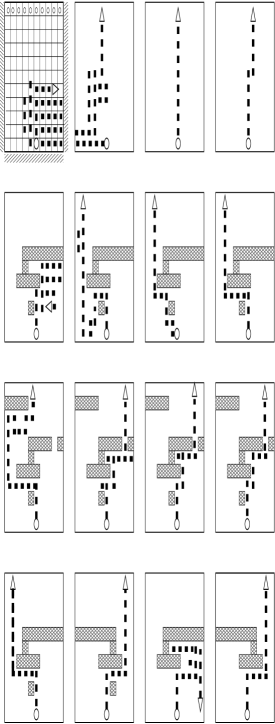
Figure 4: Typical behaviour of a simulated robot moving on various $10\times 11$ boards: the first left plot indicates the grid, the boundary walls, the starting position on the bottom line and the goal upper line. Left set of plots: The first three rows show realizations of paths taken by the robot in three different environments, “Empty board” (first row), “Right hand trap” (second row), and “Open trap” (third row) respectively. The different environments were presented to the robot in three consecutive trials, i.e., the weights are not reinitialized before a new trial. Within each row the panels represent from left to right: First run, early performance, and two different realizations of late performance. In the simulations a maximal allowed number of steps of 100 is imposed (after which the run is stopped and maximal penalty assigned). The fourth row represents two trials on pairs of configurations related by a mirror symmetry, “Traps with clue” (left pair) and “Traps without clue” (right pair). Here 120 runs are performed between switches within a pair, and the weights are not reinitialized after switches. The cutoff for the maximal number of steps is imposed at 60 for this experiment. Right set of plots: Length of the path taken to the upper line of the board, plotted run by run for the trials shown in the left set of plots. First row: “Empty board” for two settings of the randomness parameter $\beta$. The length of the best path is 10 steps in this case. Second row: “Right hand trap” (left) and “Open trap” (right), corresponding to second and third row respectively in the left set of plots. In both cases the length of the best path is 13 steps. The dotted (lower) line on the plots indicates the number of steps lost running against obstacles (this has to be added to the length of the path to give the total number of steps). Third row: performance on switching experiments for the symmetric pair of “Traps with clue” (left) and the pair of “Traps without clue” (right). The best paths have different lengths for the symmetry-related traps, viz. 13 and 11 steps for the left and right member of a trap-pair, respectively. As can be seen, the performance is much better if the situation provides a clue (left pair of traps), which means that the agent is able to “identify” it as such and use it.

Illustration 2

Consider the problem of identifying a certain pattern which is part of a sequence of different patterns – such as a certain gene in a chromosome, say. We can only know that the pattern is or is not there – e.g., from the expected expression of the gene in the phenotype. A similar problem may be that of finding the scent signature of an (unknown) unpalatable component in food: The animal tries food in various combination and can only judge about the combination as a whole. In both cases we must allow for variations of the pattern we are trying to identify (defining thus the class, say, +1). For definiteness we take sequences (bags) of 5 patterns, each pattern being itself a string of $N=20$ bits of information. We assume that a “positive” string may be contained at most once in each sequence (in a bag), and we allow about $10^{4}$ variations of it (while there are about $10^{6}$ patterns of class -1). The student is presented with sequences which contain a “positive” string with 50% probability. The student only knows (from the observation of the phenotype, from the effect of the food consumption) whether or not a class +1 string is contained in the bag. He or she therefore makes proposals on the basis of his/her momental knowledge – the synapse strengths – and then updates the latter globally taking into account whether its own conclusion matches the observation. We therefore have a particular hidden instance problem with structured data (HI-SD). In Fig. 5 we present simulation results for this system for various initial step sizes $1/\sqrt{Q(0)}$ and parameter $\lambda$ chosen to be near the corresponding thresholds. We also demonstrate that it is possible to improve the algorithm by a simple tuning of $\lambda$ with the running average ${\bar{e}}_{q}=\frac{1}{q}\sum_{q^{\prime}=0}^{q}e_{q^{\prime}}$. The beneficial effect of this tuning can in a certain sense be seen as reinforcing our claim that it is a combination of both mechanisms — the autonomous Hebbian association, and the synaptic response to evaluative feedback — which allows learning under the conditions of non-specific feedback to be successful. Tuning with the average ${\bar{e}}_{q}$ is an effective way to ensure that the balance between both mechanisms is maintained throughout the learning history, in particular in later stages with good generalization, where changes via replay become both small and rare, because $e_{q}$ will often be small or zero. Early and fast learning are thus easy to achieve: in our illustration already after a few seconds of CPU the error drops far below 1%. Again, however, we see the main interest of the learning model presented here in its simplicity and versatility in connection with understanding biological developments.

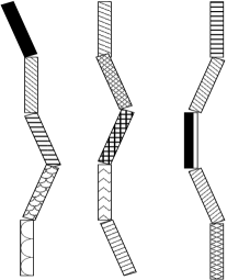
Figure 5: Looking for strings of “black” signature: length of the strings $N=20$, length of the string sequences $L=5$. $\epsilon_{G}$ vs $\alpha$ for various starting learning steps $1/\sqrt{Q(0)},\ Q(0)=50000$ (empty circles), 5000 (‘x’-s) and 50 (asterisks), and $\lambda$ near the corresponding thresholds (0.250, 0.420 and 0.560, respectively). The black circles represent the decay of the generalization error for the tuning $\lambda\propto{\bar{e}}_{q}$ ($\lambda$(0)=0.560, $Q(0)=50$).

References

- [1] Menzel, R. (2003), “Creating Presence by Bridging Between the Past and the Future: the Role of Learning and Memory for the Organization of Life”, in Kühn et al (Eds.) (2003), Adaptivity and Learning, Springer, Heidelberg, New York.
- [2] Byrne, R. (1999), The Thinking Ape, Oxford University Press, Oxford.
- [3] Mitchell, T.M. (1997) Machine Learning, Mc Graw Hill.
- [4] Sutton, R.S. and Barto, A.G. (2000), Reinforcement Learning - an Introduction, MIT Press, Cambridge, Ma.
- [5] Vapnik, V.N. (1998) Statistical Learning Theory, J.Wiley and Sons, Inc, New York.
- [6] Hertz, J., Krogh, A. and Palmer, R.G. (1991), Introduction to the Theory of Neural Computation, Addison-Wesley, Reading, Mass.
- [7] Kühn, R. and Stamatescu, I.-O. (1999), J. Phys. A: Math. Gen. 32, 5479.
- [8] Biehl, M., Kühn, R. and Stamatescu, I.-O. (2000), J. Phys. A: Math. Gen. 33, 6843.
- [9] Bergmann, U., Kühn, R. and Stamatescu, I.-O., in preparation.
- [10] Wyatt, J. (2003) “Reinforcement learning: a brief overview”, in Kühn et al. 2003.
- [11] Mlodinov, L. and Stamatescu, I.-O. (1985), Int. J. of Comp. and Inform. Sci, 14, 201.
- [12] Stamatescu, I.-O. (2003), “A simple model for learning from nonspecific reinforcement”, in Kühn et al. 2003.
- [13] Foster, D. J. and Wilson, M. A., I.-O. (1999), Nature 04587 (2006). We thank our colleague U. Bergmann for driving our attention onto this paper.
- [14] Crick, F. and Mitchison, G. (1983) The function of dream sleep, Nature 304, 111-114; Hopfield, J. J., Feinstein, D. I. and Palmer, R. G. (1983), Unlearning has a stabilizing effect in collective memories, Nature 304, 158-159; van Hemmen, J.L. (1997), Hebbian learning, its correlation catastrophe, and unlearning, Network 8, V1-V17.
- [15] Opper, M., Kinzel, W., Kleinz, J. and Nehl, R. (1990), J. Phys. A: Math. Gen. 23, L581.
- [16] Schölkopf, B. and Smola, A. (2002), Learning with Kernels, MIT Press, Cambridge Mass.
- [17] Saad, D. and Solla, S. A. (1995), Phys. Rev. Lett. 74, 4337.