Bacterial gene regulation in diauxic and nondiauxic growth

Abstract

When bacteria are grown in a batch culture containing a mixture of two growth-limiting substrates, they exhibit a rich spectrum of substrate consumption patterns including diauxic growth, simultaneous consumption, and bistable growth. In previous work, we showed that a minimal model accounting only for enzyme induction and dilution captures all the substrate consumption patterns (Narang, Biotech. Bioeng., 59, 116, 1998; Narang, J. Theoret. Biol., accepted, 2006). In this work, we construct the bifurcation diagram of the minimal model, which shows the substrate consumption pattern at any given set of parameter values. The bifurcation diagram explains several general properties of mixed-substrate growth. (1) In almost all the cases of diauxic growth, the “preferred” substrate is the one that, by itself, supports a higher specific growth rate. In the literature, this property is often attributed to the optimality of regulatory mechanisms. Here, we show that the minimal model, which contains no regulation, displays the property under fairly general conditions. This suggests that the higher growth rate of the preferred substrate is an intrinsic property of the induction and dilution kinetics. (2) The model explains the phenotypes of various mutants containing lesions in the regions encoding for the operator, repressor, and peripheral enzymes. A particularly striking phenotype is the “reversal of the diauxie” in which the wild-type and mutant strains consume the very same two substrates in opposite order. This phenotype is difficult to explain in terms of molecular mechanisms, such as inducer exclusion or CAP activation, but it turns out to be a natural consequence of the model. We show furthermore that the model is robust. The key property of the model, namely, the competitive dynamics of the enzymes, is preserved even if the model is modified to account for various regulatory mechanisms. Finally, the model has important implications for the problem of size regulation in development. It suggests that protein dilution is one mechanism for coupling patterning and growth.

url]http://narang.che.ufl.edu

1 Introduction

When microbial cells are grown in a batch culture containing a mixture of two carbon sources, they often exhibit diauxic growth (Monod, 1947). This phenomenon is characterized by the appearance of two exponential growth phases separated by a lag phase called diauxic lag. The most well-known example of the diauxie is the growth of Escherichia coli on a mixture of glucose and lactose. Early studies by Monod showed that in this case, the two exponential growth phases reflect the sequential consumption of glucose and lactose (Monod, 1942). Moreover, only glucose is consumed in the first exponential growth phase because the synthesis of the peripheral enzymes for lactose is somehow abolished in the presence of glucose. These enzymes include lactose permease (which catalyzes the transport of lactose into the cell), $\beta$-galactosidase (which hydrolyzes the intracellular lactose into products that feed into the glycolytic pathway) and lactose transacetylase (which is believed to metabolize toxic thiogalactosides transported by lactose permease). During the period of preferential growth on glucose, the peripheral enzymes for lactose are diluted to very small levels. The diauxic lag reflects the time required to build up these enzymes to sufficiently high levels. After the diauxic lag, one observes the second exponential phase corresponding to consumption of lactose.

It turns out that the peripheral enzymes for lactose are synthesized only if lactose is present in the environment. The mechanism for the synthesis or induction of these enzymes in the presence of lactose and absence of glucose was discovered by Monod and coworkers (Jacob and Monod, 1961). It was shown that the genes corresponding to these enzymes are contiguous on the DNA and transcribed in tandem, an arrangement referred to as the lac operon (Fig. 1a). In the absence of lactose, the lac operon is not transcribed because a molecule called the lac repressor is bound to a specific site on the lac operon called the operator (Fig. 1b, bottom). This prevents RNA polymerase from attaching to the operon and initiating transcription. In the presence of lactose, transcription of lac is triggered because allolactose, a product of $\beta$-galactosidase, binds to the repressor, and renders it incapable of binding to the operator (Fig. 1b, middle).

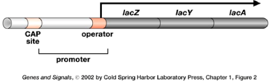
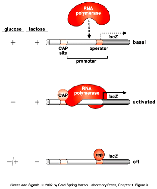
Figure 1: Molecular mechanism for induction and repression of the lac operon in E. coli  (Ptashne and Gann, 2002): (a) Structure of the lac operon. The lacZ, lacY, and lacA genes code for $\beta$-galactosidase, lactose permease, and lactose transacetylase, respectively. The operator, promoter, and CAP site denote the DNA sequences which bind the repressor, RNA polymerase, and CAP-cAMP, respectively. (b) The states of the lac operon in the presence of glucose or/and lactose. The repressor and CAP-cAMP complex are denoted rep and CAP, respectively.

The occurrence of the glucose-lactose diauxie suggests that transcription of lac is somehow repressed in the presence of glucose. Two molecular mechanisms have been proposed to explain this repression.

1. Inducer exclusion (Postma et al., 1993): In the presence of glucose, enzyme IIA^glc, a peripheral enzyme for glucose, is dephosphorylated. The dephosphorylated IIA^glc inhibits lactose uptake by binding to lactose permease. This reduces the intracellular concentration of allolactose, and hence, the transcription rate of the lac operon.
   Genetic evidence suggests that phosphorylated IIA^glc activates the enzyme, adenylate cyclase, which catalyzes the synthesis of cyclic AMP (cAMP). Since the total concentration of IIA^glc remains constant on the rapid time scale of its dephosphorylation, exposure of the cells to glucose causes a decrease in the level of phosphorylated IIA^glc, and hence, cAMP. This reduction of the cAMP level forms the basis of yet another mechanism of lac repression.

2. cAMP activation (Ptashne and Gann, 2002, Chap. 1): It has been observed that RNA polymerase is not recruited to the lac operon unless a protein called catabolite activator protein (CAP) or cAMP receptor protein (CRP) is bound to a specific site on the lac operon (denoted “CAP site” in Fig. 1). Furthermore, CAP, by itself, has a low affinity for the CAP site, but when bound to cAMP, its affinity for the CAP site increases dramatically. The inhibition of lac transcription by glucose is then explained as follows.
   In the presence of lactose alone (i.e., no glucose), the cAMP level is high. Hence, CAP becomes cAMP-bound, attaches to the CAP site, and promotes transcription by recruiting RNA polymerase (Fig. 1b, middle). When glucose is added to the culture, the cAMP level decreases by the mechanism described above. Consequently, CAP, being cAMP-free, fails to bind to the CAP site, and lac transcription is abolished (Fig. 1b, top).

We show below that neither one of these two mechanisms can fully explain the glucose-mediated repression of lac transcription.

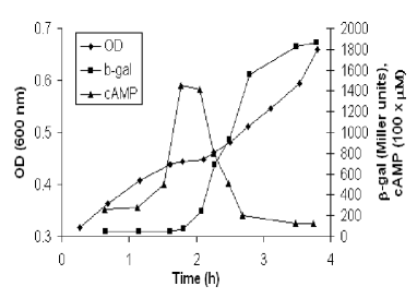
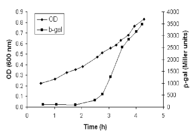
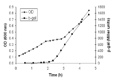
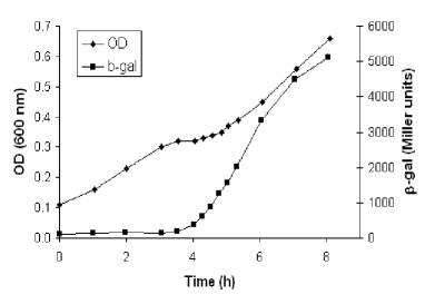
Figure 2: Repression of lac transcription in the presence of glucose is not due to reduced cAMP levels (Inada et al., 1996; Kimata et al., 1997). OD denotes optical density, and Miller units are a measure of $\beta$-galactosidase activity. (a) Growth of the wild-type strain, E. coli W3110, on glucose + lactose. The intracellular cAMP levels are comparable during the two exponential growth phases. (b) Growth of E. coli W3110 on glucose + lactose in the presence of 5 mM cAMP. Despite the high cAMP concentration, $\beta$-galactosidase synthesis is repressed during the first exponential growth phase. (c, d) Growth of E. coli $\triangle$cya crp^∗ and PR166 on glucose + lactose. The lac transcription rate in these strains is independent of the cAMP level, but $\beta$-galactosidase synthesis is repressed during the first exponential growth phase.

The following three observations contradict the cAMP activation model.

1. The intracellular cAMP levels during the first exponential growth phase ($\sim$2.5 $\mu$M) are comparable, if not higher, than those observed during the second exponential growth phase ($\sim$1.25–2 $\mu$M) (Fig. 2a).
   It follows that the repression of lac transcription in the presence of glucose is not due to lower cAMP levels.

2. When the culture is exposed to large concentrations (5 mM) of exogenous cAMP, the diauxic lag vanishes, but the lac operon still fails to be transcribed during the first exponential growth phase (Fig. 2b).
   The disappearance of the diauxic lag implies that an elevated level of intracellular cAMP does stimulate the lac transcription rate. However, it fails to relieve the repression of lac transcription in the presence of glucose.

3. Diauxic growth persists in cells which transcribe the lac operon at a rate that is independent of cAMP levels. This has been demonstrated with two types of cells (Fig. 2c,d). In E. coli $\triangle$cya crp^∗ mutants, crp, the gene coding for CAP, is mutated such that CAP binds to the CAP site even in the absence of cAMP. In E. coli PR166, the lac promoter is mutated such that RNA polymerase binds to the promoter even if there is no CAP-cAMP at the CAP site. In both cases, transcription of lac is independent of cAMP levels. Yet, $\beta$-galactosidase synthesis is still repressed during the first exponential growth phase.

These results show that higher cAMP levels do stimulate the lac transcription rate. Indeed, the 5-fold increase in cAMP levels at the end of the first exponential growth phase in Fig. 2a is characteristic of cells exposed to low concentrations (0.3 mM) of glucose (Notley-McRobb et al., 1997), and it is likely that this serves to reduce the length of the diauxic lag. However, lac transcription is repressed in the presence of glucose even if the ability of cAMP to influence lac transcription is abolished.

The persistence of the glucose-lactose diauxie in cAMP-independent cells has led to the hypothesis that inducer exclusion alone is responsible for inhibiting lac transcription (Inada et al., 1996; Kimata et al., 1997). However, inducer exclusion exerts a relatively mild effect on lactose uptake. In E. coli ML30, the activity of lactose permease is inhibited no more than $\sim$40% at saturating concentrations of glucose (Cohn and Horibata, 1959, Table 2). This partial inhibition by inducer exclusion cannot explain the almost complete inhibition of lac transcription.

Thus, despite several decades of research, no molecular mechanism has been found to fully explain the glucose-lactose diauxie in E. coli.

In the meantime, microbial physiologists have accumulated a vast body of work showing that diauxic growth is ubiquitous. It has been observed in diverse microbial species on many pairs of substitutable substrates (i.e., substrates that satisfy the same nutrient requirements) including pairs of carbon sources (Egli, 1995; Harder and Dijkhuizen, 1982; Kovarova-Kovar and Egli, 1998), nitrogen sources (Neidhardt and Magasanik, 1957), phosphorus sources (Daughton et al., 1979), and electron acceptors (Liu et al., 1998). These studies show that there is no correlation between the chemical identity of a compound and its ability to act as the preferred substrate. For instance, during growth on a mixture of glucose and an organic acid, enteric bacteria, such as E. coli, prefer glucose, whereas soil bacteria, such as Pseudomonas and Arthrobacter, prefer the organic acid (Harder and Dijkhuizen, 1976, 1982). However, there is a correlation between the maximum specific growth rate on a compound and its ability to act as a preferred substrate.

In most cases, although not invariably, the presence of a substrate permitting a higher growth rate prevents the utilization of a second, ‘poorer’, substrate in batch culture (Harder and Dijkhuizen, 1982, p. 461).

This remarkable correlation, which is reminiscent of anthropomorphic choice, is often rationalized by appealing to teleological (design-oriented) arguments. Harder & Dijkhuizen assert, for instance, that consumption of lactose is abolished in the presence of glucose because this prevents “unnecessary synthesis of catabolic enzymes in cells that already have available a carbon and energy source that allows fast growth” (Harder and Dijkhuizen, 1982, p. 463). However, there is no mechanistic explanation for this correlation.

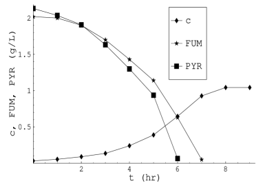
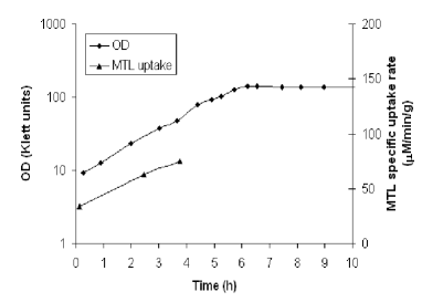
Figure 3: Simultaneous consumption of substrates in batch cultures: (a) Simultaneous consumption of fumarate (FUM) and pyruvate (PYR) during batch growth of E. coli K12 ($c$ denotes the cell density in gms dry weight per liter). The single-substrate maximum specific growth rates on fumarate and pyruvate are 0.41 h^-1 and 0.28 h^-1, respectively. This growth pattern is observed with several pairs of organic acids (Narang et al., 1997b). (b) Simultaneous consumption of glucose and mannitol (MTL) during batch growth of E. coli strain 158 (Lengeler and Lin, 1972). There is significant uptake of mannitol during the first 4 hours even though the cells are precultured on glucose.

Although the diauxie dominates the literature on mixed-substrate growth, there is ample evidence of nondiauxic growth. In E. coli K12, several pairs of organic acids are consumed simultaneously (Narang et al., 1997b), one example of which is shown in Fig. 3a. The maximum specific growth rates on these organic acids are in the range 0.28–0.44 h^-1, which are low compared to the largest maximum specific growth rate sustained in a minimal (synthetic) medium (0.74 h^-1 on glucose). Similar behavior has been observed in other species, leading Egli to conclude that

Especially combinations of substrates that support medium or low maximum specific growth rates are utilized simultaneously (Egli, 1995, p. 325).

However, a closer look at data suggests that low or medium growth rates are not necessary for simultaneous consumption. This is evident from Monod’s early studies with the so-called “A-sugars,” namely, glucose, fructose, mannitol, mannose, and sucrose (Monod, 1942, 1947). He found that in E. coli and B. subtilis, these sugars supported comparable maximum specific growth rates, but there was no diauxic lag during growth on a mixture of glucose and any one of the other A-sugars. Subsequent studies have confirmed that in some of these cases, both the substrates are consumed simultaneously (Fig. 3b). Now, in all the cases of simultaneous consumption described above, the single-substrate growth rates were comparable. Thus, it is conceivable that simultaneous consumption occurs whenever the ratio of the single-substrate growth rates is close to 1. It turns out that this condition may be necessary, but it is certainly not sufficient. Although the growth rates of Propionibacterium shermanii on glucose and lactate are identical (0.141 and 0.142 h^-1, respectively), lactate is consumed preferentially (Lee et al., 1974). Similarly, the growth rates of E. coli ML308 on glucose and fructose are comparable (0.91 and 0.73 h^-1, respectively), but glucose is consumed preferentially (Clark and Holms, 1976). Thus, current evidence suggests that the existence of comparable single-substrate growth rates is, perhaps, necessary, but not sufficient, for simultaneous consumption. It seems desirable to understand the mechanistic basis of this observation.

In addition to simultaneous substrate utilization, there is some evidence that the substrate utilization pattern can depend on the history of the preculture. Hamilton & Dawes were among the first to observe such behavior during the growth of Pseudomonas aeruginosa on a mixture of citrate and glucose (Hamilton and Dawes, 1959, 1960, 1961). Cells precultured on citrate showed diauxic growth with citrate as the preferred substrate, whereas cells precultured on glucose consumed both citrate and glucose. We observed a similar substrate consumption pattern during growth of E. coli K12 on glucose and pyruvate (Narang et al., 1997b). An entirely different preculture-dependent pattern was obtained during the growth of a pseudomonad on glucose and phenol (Panikov, 1995, Chap. 3, p. 181). When the cells were precultured on glucose, there was preferential consumption of glucose. Immediately after the exhaustion of phenol, when the cells were fully adapted to phenol, the medium was supplemented with additional glucose and phenol. Once again, there was diauxic growth, but phenol, rather than glucose, was the preferred substrate. In earlier work, we have argued that preculture-dependent growth patterns may be quite common — the lack of such data reflects the fact that the effect of preculturing was not investigated in most studies (Narang et al., 1997b). In order to facilitate their identification, it seems appropriate to determine the feasible preculture-dependent growth patterns.

The goal of this work is to seek mechanistic answers for the following questions

1. In diauxic growth, why is the maximum specific growth rate on the preferred substrate higher than that on the less preferred substrate?

2. Under what conditions are the substrates consumed simultaneously?

3. What types of preculture-dependent growth patterns are feasible?

There are numerous mechanistic models of mixed-substrate growth. Many of them are based on detailed mechanisms uniquely associated with the glucose-lactose diauxie in E. coli (Kremling et al., 2001; Santillán and Mackey, 2004; van Dedem and Moo-Young, 1973; Wong et al., 1997). These models cannot address the above questions, which are concerned with the general properties of mixed-substrate growth. Thus, one led to consider the more general models accounting for only those processes that are common to most systems of mixed-substrate growth (Brandt et al., 2004; Narang et al., 1997a; Narang, 1998a; Thattai and Shraiman, 2003). Recently, we have shown that these general models are similar inasmuch as the enzymes follow competitive dynamics in all the cases (Narang, 2006). However, the model in Brandt et al cannot capture nondiauxic growth, and the model in Thattai & Shraiman treats the specific growth rate as a fixed (constant) parameter, an assumption that is not appropriate for describing the growth of batch cultures.

In this work, we address the questions posed above by appealing to the minimal model in Narang (1998a). This model accounts for only enzyme induction and dilution, the two processes that occur in almost all systems of mixed-substrate growth. Yet, it captures all the batch growth patterns described above, and its extension to continuous cultures predicts all the steady states observed in chemostats (Narang, 1998b). Here, we show that the minimal model also provides mechanistic explanations for the foregoing questions. Specifically, we find that

1. If the induction kinetics are hyperbolic, the maximum specific growth rate on the preferred substrate is always higher than that on the less preferred substrate. The manifestation of this correlation in a minimal model containing no regulation suggests that its existence is not due to goal-oriented regulatory mechanisms, an assumption that lies at the heart of models based on optimality principles (Mahadevan et al., 2002; Kompala et al., 1986; Ramakrishna et al., 1996). It is an intrinsic property resulting from the kinetics of enzyme induction and dilution. We also find that the correlation can be violated when the induction kinetics are sigmoidal, and that the dynamics of these offending cases are consistent with the data in the literature.

2. The existence of comparable single-substrate growth rates is not sufficient for simultaneous consumption. This agrees with the data described above. However, we find that this condition is not necessary either. This is because the occurrence of simultaneous consumption depends not only on the relative growth rates, but also on the saturation constants for induction. If these saturation constants are small, there is simultaneous consumption, regardless of the relative growth rates.

We show, furthermore, that the classification of the substrate consumption patterns predicted by the model explains the phenotypes of several mutants. The most striking phenotype is the reversal of the diauxie, wherein both the wild-type and the mutant strains display diauxic growth, but consume the substrates in opposite order. This phenotype cannot be explained in terms of the standard molecular mechanisms, but turns out to be a natural consequence of the minimal model.

2 The model

Figure 4: Kinetic scheme of the minimal model (Narang, 1998a).

Fig. 4 shows the kinetic scheme of the minimal model. Here, $S_{i}$ denotes the $i^{{\rm th}}$ exogenous substrate, $E_{i}$ denotes the transport enzyme for $S_{i}$, $X_{i}$ denotes internalized $S_{i}$, and $C^{-}$ denotes all intracellular components except $E_{i}$ and $X_{i}$ (thus, it includes precursors, free amino acids, and macromolecules).

In this work, attention will be confined to growth in batch cultures. We assume that

1. The concentrations of the intracellular components, denoted $e_{i}$, $x_{i}$, and $c^{-}$, are based on the dry weight of the cells (g per g dry weight of cells, i.e., g gdw^-1). The concentrations of the exogenous substrate and cells, denoted $s_{i}$ and $c$, are based on the volume of the reactor (g/L and gdw/L, respectively). The rates of all the processes are based on the dry weight of the cells (g gdw^-1 h^-1). We shall use the term specific rate to emphasize this point.
   The choice of these units implies that if the concentration of any intracellular component, $Z$, is $z$ g gdw^-1, then the evolution of $z$ in batch cultures is given by

   $$\frac{dz}{dt}=r_{z}^{+}-r_{z}^{-}-\left(\frac{1}{c}\frac{dc}{dt}\right)z$$

   where $r_{z}^{+}$ and $r_{z}^{-}$ denote the specific rates of synthesis and degradation of $Z$ in g gdw^-1 h^-1.

2. The transport and peripheral catabolism of $S_{i}$ is catalyzed by the “lumped” system of peripheral enzymes, $E_{i}$. The specific uptake rate of $S_{i}$, denoted $r_{s,i}$, follows the modified Michaelis-Menten kinetics, $r_{s,i}\equiv V_{s,i}e_{i}s_{i}/(K_{s,i}+s_{i})$.

3. Part of the internalized substrate, denoted $X_{i}$, is converted to $C^{-}$. The remainder is oxidized to ${\rm CO_{2}}$ in order to generate energy.

   1. The conversion of $X_{i}$ to $C^{-}$ and ${\rm CO_{2}}$ follows first-order kinetics, i.e., $r_{x,i}\equiv k_{x,i}x_{i}$.

   2. The fraction of $X_{i}$ converted to $C^{-}$ is a constant (parameter), denoted $Y_{i}$. Thus, the specific rate of synthesis of $C^{-}$ from $X_{i}$ is $Y_{i}r_{x,i}$.

4. The internalized substrate also induces the synthesis of $E_{i}$.

   1. The specific synthesis rate of $E_{i}$ follows Hill kinetics, i.e., $r_{e,i}\equiv V_{e,i}x_{i}^{n_{i}}/(K_{e,i}^{n_{i}}+x_{i}^{n_{i}})$, where $n_{i}=1\textnormal{ or }2$. Kinetic analysis of the data shows that enzyme induction can be hyperbolic ($n_{i}=1$) or sigmoidal ($n_{i}=2$) (Yagil and Yagil, 1971).
      By appealing to a molecular model of induction, we can express $n_{i}$, $V_{e,i}$, and $K_{e,i}$ in terms of the parameters associated with repressor-operator and repressor-inducer binding. It is shown in Appendix A that the Yagil & Yagil model of induction implies that $n_{i}$ is the number of inducer molecules that bind to 1 repressor molecule. Furthermore, if the enzyme is inducible,

      $$V_{e,i}=\nu_{e,i}o_{t,i},\;K_{e,i}^{n_{i}}=\frac{K_{x,i}}{K_{o,i}}r_{t,i},$$ (1)

      where $\nu_{e,i}$ is the enzyme synthesis rate per unit mass of operator; $o_{t,i},r_{t,i}$ are the total concentrations of the operator and repressor (g gdw^-1), respectively; and $K_{x,i},K_{o,i}$ are the dissociation constants for repressor-inducer and repressor-operator binding, respectively.

   2. The synthesis of the enzymes occurs at the expense of the biosynthetic constituents, $C^{-}$.

   3. Enzyme degradation is negligibly small.

Given these assumptions, the mass balances yield the equations

$$\frac{ds_{i}}{dt} =-r_{s,i}c,\;r_{s,i}\equiv V_{s,i}e_{i}\frac{s_{i}}{K_{s,i}+s_{i}},$$ (2)

$$\frac{dx_{i}}{dt} =r_{s,i}-r_{x,i}-\left(\frac{1}{c}\frac{dc}{dt}\right)x_{i},r_{x,i}\equiv k_{x,i}x_{i},$$ (3)

$$\frac{de_{i}}{dt} =r_{e,i}-\left(\frac{1}{c}\frac{dc}{dt}\right)e_{i},\;r_{e,i}\equiv V_{e,i}\frac{x^{n_{i}}}{K_{e,i}^{n_{i}}+x^{n_{i}}},$$ (4)

$$\frac{dc^{-}}{dt} =(Y_{1}r_{x,1}+Y_{2}r_{x,2})-(r_{e,1}+r_{e,2})-\left(\frac{1}{c}\frac{dc}{dt}\right)c^{-}.$$ (5)

It is shown in Appendix B that since $x_{1}+x_{2}+e_{1}+e_{2}+c^{-}=1$, Eqs. (3)–(5) implicitly define the specific growth rate, denoted $r_{g}$, and the evolution of the cell density via the relations

$$\frac{dc}{dt}=r_{g}c,\;r_{g}\equiv\sum_{i=1}^{2}r_{s,i}-\sum_{i=1}^{2}(1-Y_{i})r_{x,i}.$$ (6)

Furthermore, since $x_{i}$ is small, it attains quasisteady state on a time scale of seconds, thus resulting in the simplified equations

$$\frac{ds_{i}}{dt} =-r_{s,i}c,$$ (7)

$$x_{i} \approx\frac{V_{s,i}e_{i}s_{i}/(K_{s,i}+s_{i})}{k_{x,i}},$$ (8)

$$\frac{de_{i}}{dt} =r_{e,i}-r_{g}e_{i},\;r_{e,i}\approx V_{e,i}\frac{[e_{i}s_{i}/(K_{s,i}+s_{i})]^{n_{i}}}{\bar{K}_{e,i}^{n_{i}}+[e_{i}s_{i}/(K_{s,i}+s_{i})]^{n_{i}}},\;\bar{K}_{e,i}\equiv K_{e,i}\frac{k_{x,i}}{V_{s,i}},$$ (9)

$$\frac{dc}{dt} =r_{g}c,\;r_{g}\approx Y_{1}r_{s,1}+Y_{2}r_{s,2},$$ (10)

$$c^{-} =1-x_{1}-x_{2}-e_{1}-e_{2},$$ (11)

where (8) is obtained from the quasisteady state relation, i.e., $0\approx r_{s,i}-r_{x,i}$.

We are particularly interested in the dynamics of the peripheral enzymes during the first exponential growth phase, since it is these finite-time dynamics that determine the substrate utilization pattern. If the peripheral enzymes for one of the substrates vanish during this period, there is diauxic growth; if the peripheral enzymes for both substrates persist, there is simultaneous substrate utilization.

It turns out that the motion of the enzymes during the first exponential growth phase is governed by only two equations. To see this, observe that during the first exponential growth phase, both substrates are in excess, i.e., $s_{i}\gg K_{s,i}$. Hence, even though the exogenous substrate concentrations are decreasing, the transport enzymes see a quasiconstant environment ($s_{i}/(K_{s,i}+s_{i})\approx$1), and approach the quasisteady state levels corresponding to exponential (balanced) growth. This motion is approximated by the equations

$$\frac{de_{1}}{dt} =V_{e,1}\frac{e_{1}^{n_{1}}}{\bar{K}_{e,1}^{n_{1}}+e_{1}^{n_{1}}}-\left(Y_{1}V_{s,1}e_{1}+Y_{2}V_{s,2}e_{2}\right)e_{1},$$ (12)

$$\frac{de_{2}}{dt} =V_{e,2}\frac{e_{2}^{n_{2}}}{\bar{K}_{e,2}^{n_{2}}+e_{2}^{n_{2}}}-\left(Y_{1}V_{s,1}e_{1}+Y_{2}V_{s,2}e_{2}\right)e_{2},$$ (13)

obtained from (9) by replacing $s_{i}/(K_{s,i}+s_{i})$ with 1. We shall refer to these as the reduced equations. It should be emphasized that the steady states of the reduced equations are quasisteady states of the full system of equations (see Narang et al., 1997a for a rigorous derivation of the reduced equations).

The reduced equations are formally similar to the equations of the standard Lotka-Volterra model for two competing species, namely,

$$\frac{dN_{1}}{dt} =r_{1}N_{1}(1-a_{11}N_{1}-a_{12}N_{2}),$$ (14)

$$\frac{dN_{2}}{dt} =r_{2}N_{2}(1-a_{21}N_{1}-a_{22}N_{2}),$$ (15)

where $N_{i}$ is the population density of the $i^{{\rm th}}$ species, $r_{i}$ is the (unrestricted) specific growth rate of the $i^{{\rm th}}$ species in the absence of any competition, and $a_{i1},a_{i2}$ are parameters that quantify the reduction of the unrestricted specific growth rate due to intra- and inter-specific competition (Murray, 1989). Thus, enzyme induction is the correlate of unrestricted growth, and the two dilution terms are the correlates of intra- and inter-specific competition. In what follows, we shall constantly appeal to this dynamical analogy.

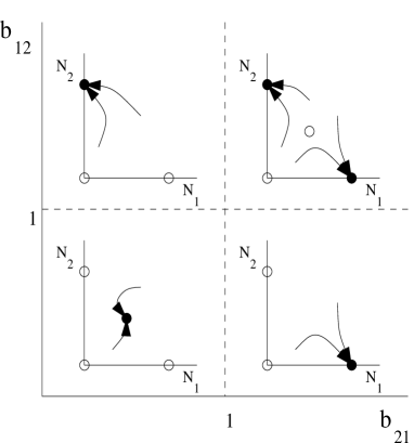
Figure 5: Classification of the global dynamics for the standard Lotka-Volterra model. The full and open circles show stable and unstable steady states, respectively.

The dynamics of the standard Lotka-Volterra model are well understood. Indeed, the bifurcation diagram of the model is completely determined by the two dimensionless parameters, $b_{21}\equiv a_{21}/a_{11}$ and $b_{12}\equiv a_{12}/a_{22}$ (Fig. 5). These parameters characterize the extent to which each species inhibits the other species relative to the extent to which it inhibits itself. Both species coexist precisely when they inhibit themselves more than they inhibit the other species, i.e., $b_{21},b_{12}<1$. Under all other conditions, coexistence is impossible. If the interaction between the species is asymmetric ($b_{21}<1,b_{12}>1$ or $b_{21}>1,b_{12}<1$), one of them is rendered extinct (species 1 and 2, respectively). If both species inhibit the other species more than they inhibit themselves, i.e. $b_{21},b_{12}>1$, the outcome depends on the initial population densities.

Given the formal similarity of the reduced equations to the Lotka-Volterra model, we expect them to display “extinction” and “coexistence” dynamics. Importantly, these dynamics have simple biological interpretations. Extinction of one of the enzymes corresponds to diauxic growth, and coexistence of both enzymes corresponds to simultaneous consumption. It is therefore clear that the bifurcation diagram for the reduced equations is a useful analytical tool. It furnishes a classification of the substrate consumption patterns, which can then be used to systematically address the questions posed in the Introduction. Our first goal is to construct this bifurcation diagram.

To minimize the number of parameters in the bifurcation diagram, we rescale the reduced equations by defining the dimensionless variables

$$\epsilon_{i}\equiv\frac{e_{i}}{\sqrt{V_{e,i}/(Y_{i}V_{s,i})}},\;\tau\equiv t\sqrt{V_{e,1}Y_{1}V_{s,1}}\;.$$

The choice of the reference variables in this scaling is suggested by the following fact: $\sqrt{V_{e,i}/(Y_{i}V_{s,i})}$ and $\sqrt{V_{e,i}Y_{i}V_{s,i}}$ are upper bounds for the enzyme level and maximum specific growth rate attained during single-substrate exponential growth on saturating concentrations of $S_{i}$. Indeed, under these conditions, the mass balance for $E_{i}$ becomes

$$0=V_{e,i}\frac{e_{i}^{n_{i}}}{\bar{K}_{e,i}^{n_{i}}+e_{i}^{n_{i}}}-Y_{i}V_{s,i}e_{i}^{2}.$$

Hence, $e_{i}<\sqrt{V_{e,i}/(Y_{i}V_{s,i})}$, and the maximum specific growth rate on $S_{i}$, denoted $r_{g,i}^{{\rm max}}$, satisfies the relation

$$r_{g,i}^{{\rm max}}\approx Y_{i}V_{s,i}e_{i}<Y_{i}V_{s,i}\sqrt{\frac{V_{e,i}}{Y_{i}V_{s,i}}}=\sqrt{Y_{i}V_{s,i}V_{e,i}}.$$

The above scaling yields the dimensionless reduced equations

$$\frac{d\epsilon_{1}}{d\tau} =\frac{\epsilon_{1}^{n_{1}}}{\kappa_{1}^{n_{1}}+\epsilon_{1}^{n_{1}}}-\left(\epsilon_{1}+\alpha\epsilon_{2}\right)\epsilon_{1},$$ (16)

$$\frac{d\epsilon_{2}}{d\tau} =\alpha\frac{\epsilon_{2}^{n_{2}}}{\kappa_{2}^{n_{2}}+\epsilon_{2}^{n_{2}}}-\left(\epsilon_{1}+\alpha\epsilon_{2}\right)\epsilon_{2},$$ (17)

with dimensionless parameters

$$\kappa_{i} \equiv \frac{\bar{K}_{e,i}}{\sqrt{V_{e,i}/(Y_{i}V_{s,i})}}=K_{e,i}k_{x,i}\sqrt{\frac{Y_{i}}{V_{s,i}V_{e,i}}}=\frac{K_{x,i}r_{t,i}k_{x,i}}{K_{o,i}}\sqrt{\frac{Y_{i}}{V_{s,i}V_{e,i}}},$$ (18)

$$\alpha \equiv \;\frac{\sqrt{V_{e,2}Y_{2}V_{s,2}}}{\sqrt{V_{e,1}Y_{1}V_{s,1}}}.$$ (19)

These dimensionless parameters have simple biological interpretations. We can view $\kappa_{i}$ as a dimensionless saturation constant for induction, and $\alpha$ as a measure of the maximum specific growth rate on $S_{2}$ relative to that on $S_{1}$.

3 Results

We wish to construct the bifurcation diagram for Eqs. (16)–(17). Since limit cycles are impossible in Lotka-Volterra models for competing species (Hirsch and Smale, 1974), it suffices to determine the steady states and their stability.

Eqs. (16)–(17) admit at most four types of steady states: The trivial steady state ($\epsilon_{1}=\epsilon_{2}=0$), the semitrivial steady states ($\epsilon_{1}>0,\epsilon_{2}=0$ and $\epsilon_{1}=0,\epsilon_{2}>0$), and the nontrivial steady state, $\epsilon_{1},\epsilon_{2}>0$. We denote these steady states by $E_{00}$, $E_{10}$, $E_{01}$, and $E_{11}$, respectively.

We shall consider two cases: $n_{1}=n_{2}=1$ and $n_{1}=2$, $n_{2}=1$. The second case will serve to show the qualitative changes engendered by sigmoidal induction kinetics.

3.1 Case 1 ($n_{1}=n_{2}=1$)

In this case, the scaled equations are

$$\frac{d\epsilon_{1}}{dt} =\frac{\epsilon_{1}}{\kappa_{1}+\epsilon_{1}}-\left(\epsilon_{1}+\alpha\epsilon_{2}\right)\epsilon_{1},$$

$$\frac{d\epsilon_{2}}{dt} =\alpha\frac{\epsilon_{2}}{\kappa_{2}+\epsilon_{2}}-\left(\epsilon_{1}+\alpha\epsilon_{2}\right)\epsilon_{2}.$$

The bifurcation diagrams for these equations are shown in Fig. 6. They were inferred from the following facts derived in Appendix C.

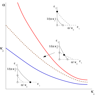
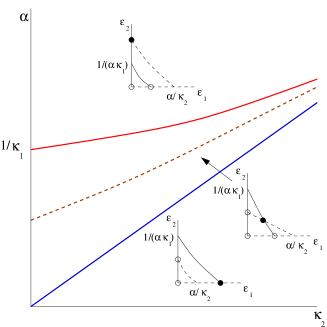
Figure 6: Bifurcation diagrams for the case $n_{1}=n_{2}=1$ at (a) fixed $\kappa_{2}>0$ and (b) fixed $\kappa_{1}>0$. In the phase portraits, the nullclines for $\epsilon_{1}$ and $\epsilon_{2}$ are represented by full and dashed lines, respectively; stable and unstable steady states are represented by full and open circles, respectively. The graphs of $\alpha_{*}$, $\alpha^{*}$, and $\alpha_{g}$ are represented by blue, red, and dashed brown curves.

1. The trivial steady, $E_{00}$, always exists (for all $\alpha,\kappa_{1},\kappa_{2}>0$), but it is always unstable (as a node).

2. The semitrivial steady state, $E_{10}$, always exists. It is (uniquely) given by

   $$\epsilon_{1}=\frac{-\kappa_{1}+\sqrt{\kappa_{1}^{2}+4}}{2},\;\epsilon_{2}=0,$$

   and is stable (as a node) precisely if $\left.\epsilon_{1}\right|_{E_{10}}$ exceeds $\alpha/\kappa_{2}$, the $\epsilon_{1}$-intercept of the nontrivial nullcline for $\epsilon_{2}$. That is

   $$\left.\epsilon_{1}\right|_{E_{10}}>\frac{\alpha}{\kappa_{2}}\Leftrightarrow\alpha<\alpha_{*}(\kappa_{1},\kappa_{2})\equiv\frac{\kappa_{2}\left(-\kappa_{1}+\sqrt{\kappa_{1}^{2}+4}\right)}{2}.$$ (20)

3. The steady state, $E_{01}$, always exists. It is given by

   $$\epsilon_{1}=0,\;\epsilon_{2}=\frac{-\kappa_{2}+\sqrt{\kappa_{2}^{2}+4}}{2},$$

   and it is stable (as a node) precisely if $\left.\epsilon_{2}\right|_{E_{01}}$ exceeds $1/(\alpha\kappa_{1})$, the $\epsilon_{2}$-intercept of the nontrivial nullcline for $\epsilon_{1}$, i.e.,

   $$\left.\epsilon_{2}\right|_{E_{01}}>\frac{1}{\alpha\kappa_{1}}\Leftrightarrow\alpha>\alpha^{*}(\kappa_{1},\kappa_{2})\equiv\frac{2}{\kappa_{1}\left(-\kappa_{2}+\sqrt{\kappa_{2}^{2}+4}\right)}.$$ (21)

4. The surface of $\alpha_{*}(\kappa_{1},\kappa_{2})$ lies below the surface of $\alpha^{*}(\kappa_{1},\kappa_{2})$, i.e.,

   $$\alpha_{*}(\kappa_{1},\kappa_{2})<\alpha^{*}(\kappa_{1},\kappa_{2})$$ (22)

   for all $\kappa_{1},\kappa_{2}>0$. The notation was chosen to reflect this fact: The functions, $\alpha_{*}(\kappa_{1},\kappa_{2})$ and $\alpha^{*}(\kappa_{1},\kappa_{2})$, represent the lower and upper surfaces of the bifurcation diagram.

5. The steady state, $E_{11}$, exists if and only if both $E_{10}$ and $E_{01}$ are unstable, i.e.,

   $$\alpha_{*}(\kappa_{1},\kappa_{2})<\alpha<\alpha^{*}(\kappa_{1},\kappa_{2}).$$ (23)

   It is unique and stable whenever it exists.

The bifurcation diagrams imply the following classification of the substrate utilization patterns.

1. If $\alpha<\alpha_{*}(\kappa_{1},\kappa_{2})$, only $E_{10}$ is stable, which corresponds to preferential consumption of $S_{1}$.

2. If $\alpha_{*}(\kappa_{1},\kappa_{2})<\alpha<\alpha^{*}(\kappa_{1},\kappa_{2})$, only $E_{11}$ is stable, and there is simultaneous consumption of $S_{1}$ and $S_{2}$.

3. If $\alpha>\alpha^{*}(\kappa_{1},\kappa_{2})$, only $E_{01}$ is stable, which corresponds to preferential consumption of $S_{2}$.

Thus, the surfaces of $\alpha_{*}(\kappa_{1},\kappa_{2})$ and $\alpha^{*}(\kappa_{1},\kappa_{2})$ delineate the boundaries of the substrate consumption patterns.

If the point, $(\kappa_{1},\kappa_{2},\alpha)$, crosses either one of these boundaries, there is an abrupt transition in the substrate consumption pattern due to transcritical bifurcations. This becomes evident if $\alpha$ is increased at any fixed $\kappa_{1},\kappa_{2}>0$ (Fig. 7). At $\alpha=\alpha_{*}(\kappa_{1},\kappa_{2})$, the substrate consumption pattern switches from preferential consumption of $S_{1}$ to simultaneous consumption of $S_{1}$ and $S_{2}$ through a transcritical bifurcation in which $E_{10}$ (red curve) yields its stability to $E_{11}$ (black curve). As $\alpha$ is increased further, there is another transition at $\alpha=\alpha^{*}(\kappa_{1},\kappa_{2})$ wherein simultaneous consumption switches to preferential consumption of $S_{2}$ via a transcritical bifurcation involving the transfer of stability from $E_{11}$ (black curve) to $E_{01}$ (blue curve).

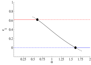
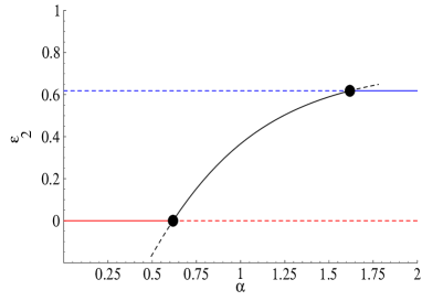
Figure 7: The bifurcation diagram obtained when $\alpha$ is increased at $\kappa_{1}=\kappa_{2}=1$. The red, blue, and black curves represent the locus of $E_{10}$, $E_{01}$, and $E_{11}$, respectively. The curves are full (resp., dashed) if the steady state is stable (resp., unstable). The bifurcation points at $\alpha=\alpha_{*}(1,1)=0.62$ and $\alpha=\alpha^{*}(1,1)=1.62$ are represented by full circles.

We gain intuitive insight into the bifurcation diagram by considering two limiting cases. Fig. 6 shows that if $\kappa_{1}$ or $\kappa_{2}$ are large, the curves for $\alpha_{*}$ and $\alpha^{*}$ converge, and simultaneous consumption is virtually impossible. In contrast, if both $\kappa_{1}$ and $\kappa_{2}$ are small, there is simultaneous consumption for almost all $\alpha$. To understand these limiting cases, observe that when $\kappa_{1},\kappa_{2}$ are large, Eqs. (16)–(17) are approximated by the equations

$$\frac{d\epsilon_{1}}{dt} \approx\frac{1}{\kappa_{1}}\epsilon_{1}\left(1-\kappa_{1}\epsilon_{1}-\alpha\kappa_{1}\epsilon_{2}\right)\epsilon_{1},$$

$$\frac{d\epsilon_{2}}{dt} \approx\frac{\alpha}{\kappa_{2}}\epsilon_{2}\left(1-\frac{\kappa_{2}}{\alpha}\epsilon_{1}-\kappa_{2}\epsilon_{2}\right)\epsilon_{2},$$

which are formally identical to the standard Lotka-Volterra model with $a_{11}=\kappa_{1}$, $a_{12}=\alpha\kappa_{1}$, $a_{21}=\kappa_{2}/\alpha$, and $a_{22}=\kappa_{2}$. However, there is an important difference. The parameters, $b_{21}\equiv a_{21}/a_{11},\;b_{12}\equiv a_{12}/a_{22}$, are not independent since $b_{21}=\kappa_{2}/(\alpha\kappa_{1})=1/b_{12}$. But if $b_{12}$ and $b_{21}$ are restricted to the curve $b_{21}b_{12}=1$, Fig. 5 implies that coexistence (i.e., simultaneous consumption) is impossible: $E_{1}$ becomes extinct if $b_{21}<1$, and $E_{2}$ becomes extinct if $b_{21}>1$. On the other hand, if $\kappa_{1},\kappa_{2}$ are small, the enzyme synthesis rate is essentially constant (quasi-constitutive). The enzymes therefore resist extinction, and coexist for almost all $\alpha$.

3.1.1 Dependence of substrate consumption pattern on genotype

In the experimental literature, the influence of the physiological parameters is often studied by altering the genetic make-up (genotype) of the cells, and observing the resultant change in the substrate consumption pattern (phenotype) of the cells. We show below that the bifurcation diagrams are consistent with the phenotypic changes observed in response to various genotypic alterations.

Before doing so, however, it is useful to note that in all the experiments described below, the phenotype of the wild-type strain is preferential consumption of a substrate (glucose, in most cases). Since Eqs. (16) and (17) are formally the same, there is no loss of generality in assuming that the preferred substrate is $S_{2}$, and the parameters, $\kappa_{1},\kappa_{2},\alpha$, for the wild-type strain lie in the region, $\alpha>\alpha^{*}$ (above the red curve in Fig. 6).

We begin by considering the cases in which the genetic perturbation transforms the substrate consumption pattern from preferential to simultaneous consumption.

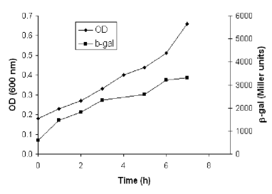
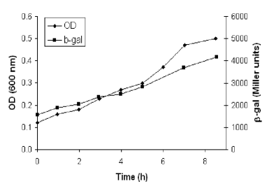
Figure 8: In E. coli PR166, synthesis of $\beta$-galactosidase persists in the presence of glucose if (a) lacY is overexpressed or (b) crr, the gene for enzyme IIA${}^{\textnormal{glc}}$, is deleted (Kimata et al., 1997). The mutant cells in (b) grow on glucose despite the absence of IIA${}^{\textnormal{glc}}$ because of slow uptake of glucose by the PTS enzymes for mannose.

In wild-type E. coli, transcription of lac is abolished in the presence of glucose. However, mutants with lesions in the lac operator synthesize $\beta$-galactosidase even in the presence of glucose (Jacob and Monod, 1961). Thus, the mutation transforms the substrate consumption pattern from preferential consumption of glucose to simultaneous consumption of glucose and lactose. The very same phenotypic change is also observed in mutants with a defective lacI, the gene encoding the lac repressor (Jacob and Monod, 1961). To explain these phenotypic changes in terms of the model, observe that mutations in the lac operator or lacI impair the lac repressor-operator binding, i.e., they increase the dissociation constant, $K_{o,1}$. It follows from Eqs. (18)–(19) that $\kappa_{1}$ decreases at fixed $\kappa_{2}$ and $\alpha$. Inspection of Fig. 6a shows that such a change can shift the substrate consumption pattern from preferential consumption of $S_{2}$ to simultaneous consumption.

If lacY, the gene encoding lactose permease, is overexpressed in E. coli PR166, synthesis of $\beta$-galactosidase persists in the presence of glucose (Fig. 8a). Now, in the model, overexpression of lacY corresponds to higher $V_{e,1}$. It follows from Eqs. (18)–(19) that $\kappa_{1},\alpha$ decrease at fixed $\kappa_{2}$, and Fig. 6a implies that the observed phenotype is indeed feasible.

In E. coli PR166, $\beta$-galactosidase is synthesized despite the presence of glucose if crr, the gene for enzyme IIA${}^{\textnormal{glc}}$, is deleted (Fig. 8a). Similarly, in the wild-type strain, E. coli K12 W3110, glucose is consumed before galactose. However, mutants with lesions in a gene encoding a transport enzyme for glucose consume the two substrates simultaneously (Kamogawa and Kurahashi, 1967). In these cases, the effect of the mutation is to decrease $V_{s,2}$, so that $\kappa_{2}$ and $\alpha$ decrease at fixed $\kappa_{1}$. It follows from Fig. 6b that such a change could lead to simultaneous consumption of the substrates.

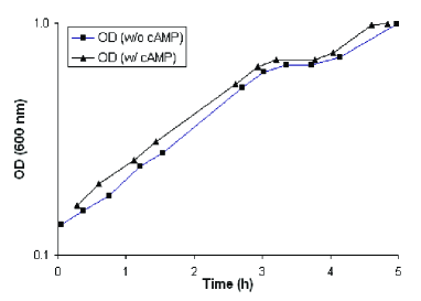
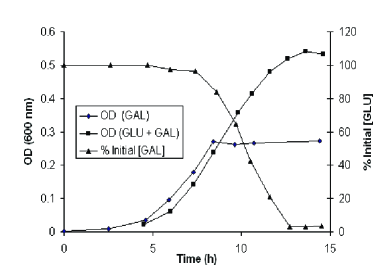
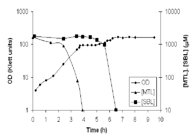
Figure 9: Reversal of the diauxie in mutants of E. coli: Upper panel: (a) In strain Hfr3000, glucose is consumed before galactose (Joseph et al., 1981). The optical density (OD) shows a pronounced diauxic lag, regardless of the presence of cAMP in the culture. (b) In the corresponding PTS-deficient strain, galactose is consumed before glucose (Asensio et al., 1963). Note that the evolution of the OD during the first 8 h is the same during growth on galactose [OD (GAL)] and glucose + galactose [OD (GLU+GAL)]. Furthermore, there is no consumption of glucose during this period. Lower panel: (c) In strain 159, mannitol (MTL) is consumed before sorbitol (SBL). (d) In the corresponding enzyme II^mtl-deficient strain, sorbitol is consumed before mannitol (Lengeler and Lin, 1972).

Now, all the mutant phenotypes discussed above can be explained just as well by alternative hypotheses appealing only to the molecular mechanisms. Indeed, the first case is obviously due to impaired repressor-operator binding, and one can argue that the remaining two cases are due to diminished inducer exclusion. However, the next two examples, which involve the reversal of the diauxie, are difficult to explain from the molecular point of view.

Fig. 9a shows that in E. coli Hfr3000, glucose is consumed before galactose. However, the mutant strain MM6, which contains a lesion in the PTS enzyme I (Tanaka et al., 1967), consumes galactose before glucose (Fig. 9b). Likewise, E. coli strain 159 consumes mannitol before sorbitol (Fig. 9c), but the corresponding mutant strain 157, which contains a lesion in the PTS enzyme II^mtl, consumes sorbitol before mannitol (Fig. 9d). These phenotypic changes fall within the scope of the minimal model. In both mutants, the transport enzyme for the preferred substrate is impaired, i.e., $V_{s,2}$ decreases, so that $\kappa_{1}$ remains unchanged, but $\kappa_{2}$ increases and $\alpha$ decreases. If the changes in $\kappa_{2}$ and $\alpha$ are sufficiently large, Fig. 6b implies that the substrate consumption pattern will shift from preferential consumption of $S_{2}$ to preferential consumption of $S_{1}$.

It should be emphasized that the “reversal of the diauxie” is a natural consequence of the minimal model. This is because each enzyme inhibits the other enzyme due to dilution by growth, i.e., the inhibition is mutual or competitive. Consequently, suppressing the uptake (and hence, the growth) on one of the substrates automatically tilts the balance of power in favor of the other substrate. In contrast, the “reversal of the diauxie” is difficult to explain in terms of molecular mechanisms alone. This is because in all the molecular mechanisms, the inhibition is unilateral rather than mutual. In E. coli, for instance, there are numerous mechanisms that allow PTS sugars, such as glucose and mannitol, to inhibit the synthesis of the enzymes for non-PTS substrates. But there is no mechanism for non-PTS substrates to inhibit the synthesis of PTS enzymes. This difficulty did not escape the attention of Asensio et al, who observed the reversal of the glucose-galactose diauxie (Fig. 9, top panel). Faced with the “reversal of the diauxie,” they were compelled to conclude that the “diauxie is, at least in part, due to competitive effects at the permease level.”

3.1.2 Dependence of substrate consumption pattern on relative growth rates

In order to consider the relationship between the substrate consumption pattern and the ratio of the single-substrate maximum specific growth rates, define

$$\rho\equiv\frac{r_{g,2}^{{\rm max}}}{r_{g,1}^{{\rm max}}},$$

where $r_{g,i}^{{\rm max}}$ denotes maximum specific growth rate during single-substrate growth on saturating concentrations of $S_{i}$. Now, the model implies that

$$r_{g,1}^{{\rm max}} =Y_{1}V_{s,1}\left.e_{1}\right|_{E_{10}}=\sqrt{V_{e,1}Y_{1}V_{s,1}}\left.\epsilon_{1}\right|_{E_{10}},$$

$$r_{g,2}^{{\rm max}} =Y_{2}V_{s,2}\left.e_{2}\right|_{E_{01}}=\sqrt{V_{e,2}Y_{2}V_{s,2}}\left.\epsilon_{2}\right|_{E_{01}},$$

so that

$$\rho=\alpha\frac{\left.\epsilon_{2}\right|_{E_{01}}}{\left.\epsilon_{1}\right|_{E_{10}}}=\frac{\alpha}{\alpha_{g}(\kappa_{1},\kappa_{2})},\;\alpha_{g}(\kappa_{1},\kappa_{2})\equiv\frac{\left.\epsilon_{1}\right|_{E_{10}}}{\left.\epsilon_{2}\right|_{E_{01}}}=\frac{-\kappa_{1}+\sqrt{\kappa_{1}^{2}+4}}{-\kappa_{2}+\sqrt{\kappa_{2}^{2}+4}}.$$

It follows that

1. The surface of $\alpha_{g}(\kappa_{1},\kappa_{2})$ separates the parameter space into two distinct regions: Above the surface, $\rho>1$, i.e., $r_{g,2}^{{\rm max}}>r_{g,1}^{{\rm max}}$, and below the surface, $\rho<1$, i.e., $r_{g,2}^{{\rm max}}<r_{g,1}^{{\rm max}}$.

2. The surface of $\alpha_{g}(\kappa_{1},\kappa_{2})$ lies between the surfaces of $\alpha_{*}(\kappa_{1},\kappa_{2})$ and $\alpha^{*}(\kappa_{1},\kappa_{2})$, i.e.,

   $$\alpha_{*}(\kappa_{1},\kappa_{2})<\alpha_{g}(\kappa_{1},\kappa_{2})<\alpha^{*}(\kappa_{1},\kappa_{2})$$ (24)

   for all $\kappa_{1},\kappa_{2}>0$ (see Appendix C). Thus, the graph of $\alpha_{g}$, denoted by the dashed brown line in Fig. 6, lies between the graphs of $\alpha_{*}$ (blue curve) and $\alpha^{*}$ (red curve).

Given these results, we can recast the classification of the substrate consumption patterns in terms of $\rho$. To this end, define

$$\rho_{*}(\kappa_{2}) \equiv\frac{\alpha_{*}(\kappa_{1},\kappa_{2})}{\alpha_{g}(\kappa_{1},\kappa_{2})}=\kappa_{2}\frac{-\kappa_{2}+\sqrt{\kappa_{2}^{2}+4}}{2},$$

$$\rho^{*}(\kappa_{1}) \equiv\frac{\alpha^{*}(\kappa_{1},\kappa_{2})}{\alpha_{g}(\kappa_{1},\kappa_{2})}=\frac{1}{\kappa_{1}}\frac{2}{-\kappa_{1}+\sqrt{\kappa_{1}^{2}+4}}.$$

Then, there is preferential consumption of $S_{1}$ (resp., $S_{2}$) precisely when $\rho<\rho_{*}(\kappa_{2})$ (resp., $\rho>\rho^{*}(\kappa_{1})$), and simultaneous consumption if and only if $\rho_{*}(\kappa_{2})<\rho<\rho^{*}(\kappa_{1})$. Thus, $\rho_{*}$ and $\rho^{*}$ define the limits of $\rho$ at which there is simultaneous consumption. It turns out that $\rho_{*}(\kappa_{2})$ increases from 0 to 1 as $\kappa_{2}$ goes from 0 to $\infty$, and $\rho^{*}(\kappa_{1})$ decreases from $\infty$ to $0$ as $\kappa_{1}$ goes from $0$ to $\infty$ (Fig. 10). We are now ready to discuss the relationship between the substrate consumption patterns and the ratio of the single-substrate maximum specific growth rates.

The Harder & Dijkhuizen correlation states that when growth is diauxic, the preferred substrate is the one that, by itself, supports a higher maximum specific growth rate (p. 1). The model predictions are consistent with this correlation. This is already evident from Fig. 6: $\alpha<\alpha_{g}$, i.e., $\rho<1$ in the region, $\alpha<\alpha_{*}$, corresponding to preferential consumption of $S_{1}$, and $\alpha>\alpha_{g}$, i.e., $\rho>1$ in the region $\alpha>\alpha^{*}$ corresponding to preferential consumption of $S_{2}$. The same property is also manifested in Fig. 10, e.g., in the region, $\rho<\rho_{*}(\kappa_{2})$, corresponding to preferential consumption of $S_{1}$, $\rho<1$ because the graph of $\rho_{*}(\kappa_{2})$ is always below 1. The manifestation of the Harder-Dijkhuizen correlation in this minimal model suggests that is an intrinsic property of the induction and dilution kinetics. It can be explained without invoking goal-oriented regulatory mechanisms, which form the basis of models based on optimality principles (Kompala et al., 1986; Mahadevan et al., 2002; Ramakrishna et al., 1996).

Figure 10: Classification of substrate consumption patterns in terms of $\rho$, the ratio of the single-substrate maximum specific growth rates. The full and dashed lines show the graphs of $\rho_{*}(\kappa_{2})$ and $\rho^{*}(\kappa_{1})$, respectively.

Current experimental evidence suggests that the existence of comparable single-substrate maximum specific growth rates is, perhaps, necessary but not sufficient for simultaneous consumption (p. 4). However, Fig. 10 shows that this condition ($\rho\approx 1$) is neither necessary nor sufficient for simultaneous consumption. It is not necessary because when $\kappa_{1},\kappa_{2}\ll 1$, there is simultaneous consumption for almost all $\rho$. It is not sufficient for simultaneous consumption because when $\kappa_{1},\kappa_{2}\gg 1$, simultaneous consumption is virtually impossible — it cannot be obtained unless $\rho$ lies in a vanishingly small neighborhood of 1. These results can be understood in terms of the limiting cases discussed above. If $\kappa_{1},\kappa_{2}$ are small, the enzymes are quasi-constitutive, and they resist extinction, regardless of the maximum specific growth rates. As $\kappa_{1}$ and $\kappa_{2}$ increase, the enzymes become progressively more vulnerable to extinction, and in the limit of large $\kappa_{1},\kappa_{2}$, they cannot coexist.

We note finally that unlike the standard Lotka-Volterra model for competing species, there are no parameter values that yield bistable enzyme dynamics (compare Figs. 5 and 6). We show below that bistability becomes feasible when the induction kinetics are sigmoidal.

3.2 Case 2 ($n_{1}=2,\;n_{2}=1$)

In this case, the scaled equations are

$$\frac{d\epsilon_{1}}{dt} =\frac{\epsilon_{1}^{2}}{\kappa_{1}^{2}+\epsilon_{1}^{2}}-\left(\epsilon_{1}+\alpha\epsilon_{2}\right)\epsilon_{1}$$

$$\frac{d\epsilon_{2}}{dt} =\alpha\frac{\epsilon_{2}}{\kappa_{2}+\epsilon_{2}}-\left(\epsilon_{1}+\alpha\epsilon_{2}\right)\epsilon_{2}$$

The key results, which are shown in detail in Appendix D, are as follows

1. The trivial steady, $E_{00}$, always exists, regardless of the parameter values. It is always unstable.

2. The semitrivial steady state, $E_{10}$, exists if and only if $\kappa_{1}<1$, in which case it is unique, and given by

   $$\epsilon_{1}=\sqrt{1-\kappa_{1}^{2}},\;\epsilon_{2}=0.$$

   It is stable (as a node) if and only if $\left.\epsilon_{1}\right|_{E_{10}}$ exceeds the $\epsilon_{1}$-intercept of the nontrivial nullcline for $\epsilon_{2}$, i.e.,

   $$\left.\epsilon_{1}\right|_{E_{10}}>\frac{\alpha}{\kappa_{2}}\Leftrightarrow\alpha<\kappa_{2}\sqrt{1-\kappa_{1}^{2}}\equiv\alpha_{*}(\kappa_{1},\kappa_{2}).$$ (25)

3. The semitrivial steady state, $E_{01}$, always exists, and is given by

   $$\epsilon_{1}=0,\;\epsilon_{2}=\frac{-\kappa_{2}+\sqrt{\kappa_{2}^{2}+4}}{2}.$$ (26)

   It is always stable (as a node).

4. Nontrivial steady states exist only if $\kappa_{1}<1$. Under these conditions, there are at most two nontrivial steady states. There is a unique nontrivial steady state if and only if

   $$0<\alpha<\alpha_{*}(\kappa_{1},\kappa_{2}),$$

   and it is unstable whenever it exists. There are two nontrivial steady states if and only if

   $$0<\kappa_{1}<\beta\equiv\sqrt{\frac{2+\kappa_{2}^{2}}{2(1+\kappa_{2}^{2})}},\;\alpha_{*}(\kappa_{1},\kappa_{2})<\alpha<\alpha^{*}(\kappa_{1},\kappa_{2}),$$

   where $\alpha^{*}(\kappa_{1},\kappa_{2})$ is the value of $\alpha$ at which the nontrivial nullclines for $\epsilon_{1}$ and $\epsilon_{2}$ touch. One of these steady states is stable and the other is unstable.

5. The surface of $\alpha_{*}(\kappa_{1},\kappa_{2})$ lies below the surface of $\alpha^{*}(\kappa_{1},\kappa_{2})$ for all $0<\kappa_{1}<\beta$ and $\kappa_{2}>0$.

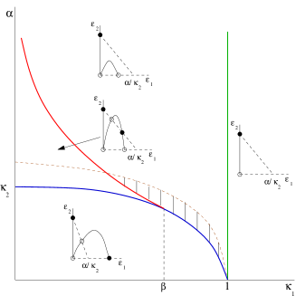
Figure 11: The bifurcation diagram for the case $n_{1}=2$, $n_{2}=1$ at any fixed $\kappa_{2}>0$. In the phase portraits, the nullclines for $\epsilon_{1}$ and $\epsilon_{2}$ are represented by full and dashed lines, respectively; stable and unstable steady states are represented by full and open circles, respectively. The graphs of $\alpha_{*}$, $\alpha^{*}$, $\kappa_{1}=1$, and $\alpha_{g}$ are represented by blue, red, green, and dashed brown curves, respectively. In the hatched region, $S_{2}$ is the preferred substrate for all preculturing conditions, even though it supports a maximum specific growth rate lower than that on $S_{1}$.

The bifurcation diagram shown in Fig. 11 implies the following classification of the substrate utilization patterns.

1. If $\alpha<\alpha_{*}$, $E_{10}$ and $E_{01}$ are stable, i.e., there is preferential consumption of $S_{1}$ or $S_{2}$, depending on the initial conditions.

2. If $0<\kappa_{1}<\beta$ and $\alpha_{*}<\alpha<\alpha^{*}$, $E_{01}$ and $E_{11}$ are stable, i.e., there is preferential consumption of $S_{2}$ or simultaneous consumption of $S_{1}$ and $S_{2}$, depending on the initial conditions.

3. If $\beta<\kappa_{1}<1,\alpha>\alpha_{*}$ or $\kappa_{1}>1$, there is preferential consumption of $S_{2}$, regardless of the initial conditions.

The surfaces of $\alpha_{*}$ and $\alpha^{*}$ define the locus of transcritical and fold (saddle-node) bifurcations, respectively (Fig. 12). If $\alpha$ is increased at any fixed $0<\kappa_{1}<\beta$ and $\kappa_{2}>0$, the substrate consumption pattern changes at $\alpha=\alpha_{*}$ from bistable dynamics involving preferential consumption of $S_{1}$ or $S_{2}$ to bistable dynamics involving preferential consumption of $S_{2}$ or simultaneous consumption. This transition occurs via a transcritical bifurcation. At $\alpha=\alpha^{*}$, the substrate consumption pattern switches to preferential consumption of $S_{2}$ via a fold bifurcation.

Comparison of Fig. 11 with Fig. 6 shows that certain features are preserved. Specifically, preferential consumption of $S_{1}$ is feasible only at low $\alpha$, and simultaneous consumption occurs only if $\alpha$ has intermediate values and $\kappa_{1},\kappa_{2}$ are not too large. However, a unique property emerges in Fig. 11, namely, bistability. This is due to the sigmoidal induction kinetics for $E_{1}$, which ensure that preferential consumption of $S_{2}$ is feasible at all parameter values.

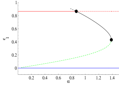
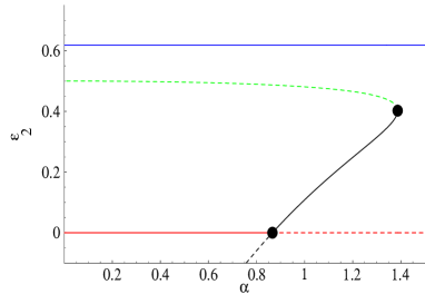
Figure 12: The bifurcation diagram obtained when $\alpha$ is increased at $\kappa_{1}=0.5$ and $\kappa_{2}=1$. The red and blue curves show the semitrivial steady states, $E_{10}$, $E_{01}$, respectively. The green and black curves show the two nontrivial states ($E_{11}$). The curves are full (resp., dashed) if the corresponding steady state is stable (resp., full). The bifurcation points are represented by full circles.

It is also worth examining the relationship between the classification predicted by the model and the empirical classification based on the single-substrate maximum specific growth rates. In this case

$$\rho=\alpha\frac{\left.\epsilon_{2}\right|_{E_{01}}}{\left.\epsilon_{1}\right|_{E_{10}}}=\frac{\alpha}{\alpha_{g}(\kappa_{1},\kappa_{2})},\;\alpha_{g}\equiv\frac{2\sqrt{1-\kappa_{1}^{2}}}{-\kappa_{2}+\sqrt{\kappa_{2}^{2}+4}}.$$

Now, $\alpha_{g}>\alpha_{*}$ because $-\kappa_{2}+\sqrt{\kappa_{2}^{2}+4}<2/\kappa_{2}$ (see Appendix C). Furthermore, $\alpha_{g}$ is zero at $\kappa_{1}=1$. Thus, the graph of $\alpha_{g}$ lies above the graph of $\alpha_{*}$ (dashed brown line in Fig. 11). This implies that a substrate can be consumed preferentially even if it supports a lower maximum specific growth rate. Indeed, if the parameters lie in the region, $\alpha<\alpha_{g}$, then $S_{2}$ supports a lower maximum specific growth rate than $S_{1}$, and yet, cells precultured on $S_{2}$ consume this substrate preferentially. If the parameter values lie in the hatched region of Fig. 11, $S_{2}$ is the preferred substrate, regardless of the manner in which the cells are precultured.

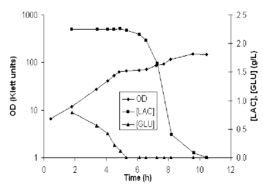
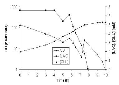
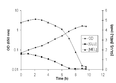
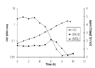
Figure 13: Bistability in mixed-substrate growth: Upper panel: Growth of Streptococcus mutans GS5 on a mixture of lactose (LAC) and glucose (GLU) (Liberman and Bleiweis, 1984). (a) Glucose is consumed preferentially if the cells are precultured on glucose. (b)  Glucose and lactose are consumed simultaneously if the cells are precultured on lactose. Lower panel: Growth of Salmonella typhimurium SB1476 on a mixture on a mixture of glucose (GLU) and melibiose (MEL) (Kuroda et al., 1992). (c) Glucose-precultured cells consume glucose before melibiose. (d) Melibiose-precultured cells consume melibiose before glucose. In (b) and (d), the concentration of glucose increases at $t\approx 8$ and $t\approx 6$ h, respectively. It is believed that is due to expulsion of the glucose produced from intracellular hydrolysis of lactose and melibiose, respectively.

3.2.1 Evidence of bistable substrate consumption patterns

The bistable dynamics predicted by Fig. 11 have been observed in experiments.

The bistable dynamics in the region, $\alpha_{*}<\alpha<\alpha^{*}$, correspond to preferential consumption of $S_{2}$ if the preculture is grown on $S_{2}$, and simultaneous consumption if the preculture is grown on $S_{1}$. Two examples of this substrate consumption pattern were described in the Introduction, namely, growth of P. aeruginosa on glucose plus citrate (Hamilton and Dawes, 1959, 1960, 1961) and growth of E. coli K12 on a mixture of glucose and pyruvate (Narang et al., 1997b). Fig. 13 shows another example of this substrate consumption pattern. When Streptococcus mutans GS5 is grown on a mixture of glucose and lactose, glucose-precultured cells consume glucose before lactose (Fig. 13a), whereas lactose-precultured cells consume both glucose and lactose (Fig. 13b).

The bistable dynamics in the region, $\alpha<\alpha_{*}$, correspond to preferential consumption of $S_{1}$ if the preculture is grown on $S_{1}$, and preferential consumption of $S_{2}$ if the preculture is grown on $S_{2}$. Furthermore, the maximum specific growth on $S_{2}$ is lower than that on $S_{1}$. There is evidence suggesting the existence of this substrate consumption pattern. Tsuchiya and coworkers studied the growth of Salmonella typhimurium on a mixture of glucose and melibiose (Kuroda et al., 1992; Okada et al., 1981). They found that the wild-type strain LT2 consumed glucose before melibiose. However, the PTS enzyme I mutant, SB1476, yielded the bistable substrate consumption pattern corresponding to the region, $\alpha<\alpha_{*}$. Cells precultured on glucose consumed glucose preferentially (Fig. 13c), and cells precultured on melibiose consumed melibiose preferentially (Fig. 13d). Moreover, the maximum specific growth rate on glucose (0.24 h^-1) is significantly lower than that on melibiose (0.41 h^-1). It should be noted that these experiments were done in the presence of 5 mM cAMP in the culture. However, at least in the case of glucose-precultured cells, the same phenotype was observed even in the absence of cAMP.

4 Discussion

We have shown that a minimal model accounting for only enzyme induction and dilution captures and explains all the substrate consumption patterns observed in the experimental literature. In what follows, we discuss the robustness of the model, and its implications for the problem of size regulation in development.

4.1 Robustness of the model

Given the simplicity of the model, it is necessary ask whether the properties of the model will be preserved if additional metabolic details and regulatory mechanisms are incorporated in the model. Now, the defining property of the minimal model is that the enzymes follow competitive dynamics. We show below that this property is not a consequence of the particular kinetics assumed in the model. It is the outcome of two very general characteristics possessed by most systems of mixed-substrate growth.

To see this, it is useful to consider the generalized Lotka-Volterra model for competing species (Hirsch and Smale, 1974, Chap. 12). This model postulates that the competitive interactions between two species are captured by the relations

$$\frac{dN_{i}}{dt}=f_{i}(N_{1},N_{2}),\;f_{1}(0,N_{2})=f_{2}(N_{1},0)=0\textnormal{ and }\;\frac{\partial f_{1}}{\partial N_{2}},\frac{\partial f_{2}}{\partial N_{1}}<0.$$

In other words, the essence of competitive interactions can be distilled into two properties:

1. The growth of a species is impossible in the absence of that species ($dN_{i}/dt=0$ whenever $N_{i}=0$).

2. Each species inhibits the growth of the other species ($\partial f_{1}/\partial N_{2},\partial f_{2}/\partial N_{1})<0$.

These properties, by themselves, imply the existence of all the dynamics associated with competitive interactions, namely, the absence of limit cycles, and the existence of extinction and coexistence steady states.

Now, properties (a) and (b) will be manifested in most systems of mixed-substrate growth. Indeed, the evolution of the enzymes during the first exponential growth phase can be described by the relations

$$\frac{de_{i}}{dt}=g_{i}(e_{1},e_{2})\equiv r_{e,i}(e_{1},e_{2})-r_{g}(e_{1},e_{2})e_{i}.$$

If we assume that

1. each enzyme is necessary for its own synthesis, i.e., $r_{e,i}=0$ whenever $e_{i}=0$,

2. each enzyme has either no effect or inhibits the synthesis of the other enzyme, i.e., $\partial r_{e,1}/\partial e_{2}$, $\partial r_{e,2}/\partial e_{1}\leq 0$,

3. the specific growth rate is an increasing function of $e_{1}$ and $e_{2}$, i.e., $\partial r_{g}/\partial e_{1}$, $\partial r_{g}/\partial e_{2}>0$,

then the enzymes satisfy both the hypotheses of the generalized model for competing species: (a) There is no enzyme synthesis in the absence of the enzyme ($de_{i}/dt=0$ whenever $e_{i}=0$), and (b) each enzyme inhibits the synthesis of the other enzyme ($\partial g_{1}/\partial e_{2}$, $\partial g_{2}/\partial e_{1}<0$). Consequently, they will display extinction and coexistence dynamics.

It remains to consider the generality of assumptions 1–3.

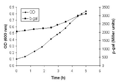
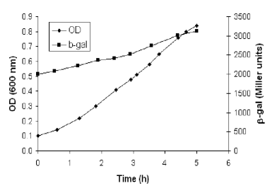
Figure 14: Disappearance of the diauxie when the enzymes are not necessary for their own synthesis (Inada et al., 1996). Synthesis of $\beta$-galactosidase persists in the presence of glucose if (a) lacI is mutated so that lac transcription becomes constitutive or (b) IPTG is present in the medium. In the first case, lac transcription is constitutive, i.e., it persists even in the absence of the inducer. In the second case, lac transcription is no longer dependent on the existence of the permease.

Assumption 1 will be satisfied whenever the substrates are transported by unique inducible enzymes. In these cases, the enzymes are required for the existence of the inducer ($e_{i}=0\Rightarrow x_{i}=0$), and the inducers are necessary for the synthesis of the enzymes ($x_{i}=0\Rightarrow r_{e,i}=0$); hence, $e_{i}=0\Rightarrow r_{e,i}=0$. One can imagine two cases in which assumption 1 is violated. First, if an enzyme is constitutive, it is synthesized even in the absence of the inducer ($x_{i}=0\nRightarrow r_{e,i}=0$). Second, in the presence of a gratuitous inducer, such as IPTG, which can enter the cell even in the absence of lactose permease, the enzyme is not required for the existence of the inducer ($e_{i}=0\nRightarrow x_{i}=0$). In both cases, the “extinction” steady state ceases to exist, and the substrates will be consumed simultaneously. This is consistent with experiments (Fig. 14).

Assumption 2 will be satisfied provided the enzymes do not activate each other. But all the known regulatory mechanisms invariably entail direct or indirect inhibition of one of the enzymes by the other enzyme. This includes inducer exclusion (dephosphorylated enzyme II^glc inhibits lac permease), and cAMP activation (dephosphorylation of II^glc causes a reduction of cAMP levels, which in turn inhibits lac transcription).

Assumption 3 will be satisfied if the yield of biomass on a substrate during single-substrate growth does not change markedly during mixed-substrate growth. In the model, the yields were assumed to be constant. This is certainly true for conservative substrates since $Y_{i}=1$. It is also observed to hold in many mixtures of carbon sources (Egli et al., 1982; Narang et al., 1997b). However, it is conceivable that there are systems in which the yields vary with the enzyme levels. In such cases, the specific growth rate will have the form, $r_{g}(e_{1},e_{2})=Y_{1}(e_{1},e_{2})V_{s,i}e_{1}+Y_{2}(e_{1},e_{2})V_{s,2}e_{2}$. At present, the data is not sufficient for determining the extent to which the yields with the enzyme levels.

It is therefore clear that inclusion of various regulatory mechanisms will enhance the mutual inhibition due from dilution. However, the qualitative behavior will be preserved, since the enzymes will still follow Lotka-Volterra dynamics. Thus, the key property of the model, namely, competitive dynamics of the enzymes, is quite robust insofar as the perturbations with respect to regulatory mechanisms are concerned.

The notion that diauxic growth is the outcome of competitive interactions between the enzymes is not new. It can be found in the earliest papers on diauxic growth. In 1947, Monod noted that (Monod, 1947, p. 254)

“it appears that the mechanisms involved in diauxic inhibition have the character of competitive interactions between different specific enzyme-forming systems.”

He observed, furthermore, that the (Monod, 1947, p. 259).

“existence of competitive interactions in the synthesis of different specific enzymes appears to be a fact of fundamental significance in enzymatic adaptation, and one for which any conception of the phenomenon should be able to account.”

However, these conclusions were based on the kinetics of the enzyme levels during diauxic growth, and had no mechanistic basis.

The above argument, first made in Narang (1998a), shows the mechanistic basis of the competitive interactions in a mathematically precise fashion.

4.2 Implication of the model for development

Diauxic growth has played a critical role in shaping models of patterning in development. The first link between genetics and development was established in the late 40’s by appealing to the following argument (Gilbert, 2002). During diauxic growth, cells possessing identical genes synthesize different proteins at distinct times (namely, the first and second exponential growth phases). By analogy, patterning in differentiation could be viewed as the synthesis of different proteins at distinct times and locations (Monod, 1947; Spiegelman, 1948). From this standpoint, diauxic growth and developmental patterning can be viewed as “temporal” and “spatiotemporal” differentiation, respectively.

The subsequent discovery of the molecular mechanisms involved in developmental patterning have confirmed the above hypothesis. It has been found that developmental patterns are generated by mechanisms similar in principle, but more complex in detail, than those involved diauxic growth (Ptashne and Gann, 2002, Chap. 3).

Despite remarkable successes in developmental patterning, there are outstanding questions about size regulation, i.e., the mechanisms by which patterning is coupled to growth (Day and Lawrence, 2000; Hafen and Stocker, 2003; Serrano and O’Farrell, 1997). Examples of such questions include: What determines the size of organs and organisms, i.e., why does their growth cease at a certain time? And why is development scale-invariant, i.e., why is the size of the organs is proportional to the size of the organism?

The model presented here may be relevant to the problem of size regulation. It shows that the “temporal” differentiation in the diauxie is coupled to growth, and this coupling is mediated by the process of enzyme dilution. Inasmuch as the diauxie is a paradigm of the mechanisms controlling cellular differentiation, a similar mechanism may lie at the heart of the coupling between developmental patterning and growth. Based on the minimal model, one can speculate, for instance, that organ growth ceases at a certain time because growth-promoting enzymes are driven to “extinction” at sufficiently high growth rates.

The model also has implications for the problem of scale invariance. In many mathematical models of development, pattern formation occurs when a homogeneous steady state of a reaction-diffusion system

$$\frac{\partial c}{\partial t}=D\nabla^{2}c-r(c,p)$$ (27)

becomes unstable due to the onset of a Turing instability (Murray, 1989). Here, $c(x,t)$ denotes the vector of morphogen concentrations, $D$ is the matrix of diffusivities, and $r(c,p)$ is the reaction rate vector expressed as a function of $c$ and a vector of parameters, $p$. In general, the patterns predicted by these models are not scale-invariant. However, this problem can be resolved if the system is fed more information about its size (say, $L$). For instance, perfect scale invariance is obtained if the diffusivities or rate constants are proportional to $L^{2}$, and plausible mechanisms for such a dependence have been proposed (Othmer and Pate, 1980; Ishihara and Kaneko, 2006).

In growing systems, however, information regarding the growth rate is constantly fed to the mechanism driving pattern formation. Indeed, in the presence of growth, Eq. (27) becomes

$$\frac{\partial c}{\partial t}+v.\nabla c=D\nabla^{2}c-r(c,p)-c\nabla\cdot v$$ (28)

where $v(x,t)$ is the velocity vector field, $v\cdot\nabla c$ is the accumulation of the morphogens due to convection, $\nabla\cdot v$ is the specific growth rate, and $c\nabla\cdot v$ is the dilution of the morphogens due to growth. Crampin et al have shown that these equations exhibit a certain degree of scale invariance — as the system grows, the number of pattern elements remains the same despite a doubling of the system size (Crampin et al., 1999, 2002). Further analysis of this class of equations offers the promise of deeper insights into the coupling between patterning and growth.

5 Conclusions

1. We showed that a minimal model accounting for enzyme induction and dilution, but not cAMP activation and inducer exclusion, captures and explains all the observed substrate consumption patterns, including diauxic growth, simultaneous consumption, and bistable growth. This suggests that the dynamics characteristic of mixed-substrate growth are already inherent in the minimal structure associated with induction and dilution. We find that many of the molecular mechanisms, such as inducer exclusion, serve to amplify these inherent dynamics.

2. We constructed bifurcation diagrams showing the parameter values at which the various substrate consumption patterns will be observed. The bifurcation diagrams explain the phenotypic responses to various genetic perturbations, including lesions in the genes for the repressor, operator, and the transport enzymes. Importantly, they provide a simple explanation for the “reversal of the diauxie,” a phenomenon which is quite difficult to explain in terms of molecular mechanisms. The bifurcation diagrams also provide deep insights into the mechanisms underlying the empirically observed correlations between the substrate consumption patterns and the single-substrate growth rates. We found that

   1. When the induction kinetics are hyperbolic, the preferred substrate is always the one that that supports a higher growth rate. This correlation is, therefore, unlikely to be the outcome of optimal design. It is a natural consequence of the fact that the enzymatic dynamics are governed by the rates of induction and dilution.
      If induction is sigmoidal, it is possible for the preferred substrate to support a lower growth rate than the less preferred substrate. We presented experimental data illustrating this case.

   2. The existence of comparable growth rates is neither necessary nor sufficient for simultaneous consumption. When the saturation constants are small, simultaneous consumption occurs regardless of the maximum specific growth rates, since induction is quasi-constitutive. If the saturation constants are large, simultaneous consumption is impossible even if the growth rates are comparable.

3. The key property of the model, namely, competitive dynamics of the enzymes, is quite robust with respect to structural perturbations.

4. The model may have implications for the problem of size regulation in development, since it provides a mechanism for coupling differentiation and growth, namely, protein dilution.

Appendix A Interpretation of $n_{i}$, $V_{e,i}$, and $K_{e,i}$ in terms of molecular interactions

To express $n_{i}$, $V_{e,i}$, and $K_{e,i}$ in terms of molecular parameters, we appeal to the Yagil & Yagil model (Yagil and Yagil, 1971). For notational clarity, we shall ignore the subscript $i$ for the substrate; thus, the operator, inducer, and repressor will be denoted by $O$, $X$, and $R$, respectively. Furthermore, their concentrations will be denoted $[O]$, $[X]$, and $[R]$, respectively.

The Yagil & Yagil model views induction as the outcome of a competition for the repressor between the operator and the inducer. Induction occurs when the inducer molecules sequester the repressors away from the operator. The competitive interactions are represented by two binding equilibria

$$R+O \rightleftharpoons R\cdot O,\;K_{o}\equiv\frac{[R][O]}{[R\cdot O]},$$ (29)

$$R+nX \rightleftharpoons R\cdot X_{n}\;K_{x}\equiv\frac{[R][X]}{[R\cdot X_{n}]},$$ (30)

where $n$ denotes the number of inducer molecules that bind to 1 molecule of repressor; $[R\cdot O]$, $[R\cdot X_{n}]$ denote the concentrations of the complexes, $R\cdot O$, $R\cdot X_{n}$, respectively; and $K_{o}$, $K_{x}$ denote the dissociation constants for the two equilibria.

It is assumed that

1. Enzyme synthesis is limited by the transcription rate, i.e., translation is not limiting. Thus, the specific enzyme synthesis rate is proportional to the specific transcription rate. Furthermore, the specific transcription rate is proportional to the concentration of the free operator, i.e.,

   $$r_{e}=\nu[O],$$ (31)

   where $\nu$ denotes the enzyme synthesis rate per unit mass of operator.

2. The total concentrations of $O$ and $R$, denoted $[O]_{t}$ and $[R]_{t}$, respectively, are conserved, i.e.,

   $$[O]_{t} =[O]+[R\cdot O],$$ (32)

   $${}[R]_{t} =[R]+[R\cdot O]+[R\cdot X_{n}].$$ (33)

   These two relations, together with Eqs. (29)–(30), constitute 4 equations in 4 unknowns, namely, $[O]$, $[R]$, $[R\cdot$O], and $[R\cdot X_{n}]$. In principle, these equations can be solved for $[O]$, and substituted in (31) to obtain $r_{e}$. However, since the solution is cumbersome, it is convenient to make the following additional assumption.

3. The repressor is bound primarily to the inducer (rather than the operator), i.e.,

   $$[R\cdot O]\ll[R\cdot X_{n}].$$

   This assumption is valid under most conditions because the operator concentration ($\sim$2 per cell) is significantly smaller than the inducer concentration.

These assumptions yield

$$r_{e}=\nu[O]=V_{e}\frac{K_{x}+[X]^{n}}{K_{x}(1+[R]_{t}/K_{o})+[X]^{n}},$$

where $V_{e}\equiv\nu[O_{t}]$.

In the case of constitutive enzymes, the repressor has a weak affinity for the operator, i.e., $K_{o}\gg[R]_{t}$, so that

$$r_{e}\approx V_{e}$$

regardless of the inducer concentration.

In the case of inducible enzymes, the repressor has a high affinity for the operator, i.e., $K_{o}\ll[R]_{t}$, so that

$$r_{e} \approx V_{e}\frac{K_{x}+[X]^{n}}{K_{x}[R]_{t}/K_{o}+[X]^{n}}.$$

This is a monotonically increasing function of $[X]$ with a small nonzero intercept. Neglecting this small “basal” enzyme synthesis rate yields

$$r_{e}\approx V_{e}\frac{[X]^{n}}{K_{e}^{n}+[X]^{n}},\;K_{e}^{n}\equiv\frac{K_{x}}{K_{o}}[R]_{t}.$$

Appendix B Derivation of the equations

Equations (3–5) implicitly define the specific growth rate and the evolution of the cell density. To see this, observe that since all the intracellular concentrations are expressed as mass fractions (g/gdw), their sum equals 1, i.e., $x_{1}+x_{2}+e_{1}+e_{2}+c^{-}=1$. Hence, addition of equations (3–5) yields

$$0=\sum_{i=1}^{2}r_{s,i}-\sum_{i=1}^{2}(1-Y_{i})r_{x,i}-\frac{1}{c}\frac{dc}{dt}$$

which can be rewritten in the more familiar form

$$\frac{dc}{dt}=r_{g}c,\;r_{g}\equiv\sum_{i=1}^{2}r_{s,i}-\sum_{i=1}^{2}(1-Y_{i})r_{x,i}$$

where $r_{g}$ denotes the specific growth rate.

We can simplify the model by observing that $x_{i}\sim 10^{-3}$ g/gdw (Chung and Stephanopoulos, 1996) and $r_{s,i},r_{x,i}\sim 1$ g gdw^-1 h^-1. Thus, $x_{i}$ attains quasisteady state on a time scale of $10^{-3}$ h. Moreover, the dilution term $r_{g}x_{i}\sim 10^{-4}$ g gdw^-1 h^-1 is negligibly small compared to $r_{s,i},r_{x,i}$. Hence, within a few seconds, (3) becomes, $0\approx r_{s,i}-r_{x,i}$, which implies that $r_{g}\approx\sum_{i}Y_{i}r_{s,i}$, i.e., $Y_{i}$ is essentially the yield of biomass on $S_{i}$. Thus, we arrive at the equations

$$\frac{dc}{dt} =(Y_{1}r_{s,1}+Y_{2}r_{s,2})c,$$

$$\frac{ds_{i}}{dt} =-r_{s,i}c$$

$$\frac{de_{i}}{dt} =r_{e,i}-(Y_{1}r_{s,1}+Y_{2}r_{s,2})e_{i},$$

$$x_{i} \approx\frac{V_{s,i}e_{i}s_{i}/(K_{s,i}+s_{i})}{k_{x,i}}$$

$$c^{-} =1-x_{1}-x_{2}-e_{1}-e_{2}$$

where $x_{i}$ is obtained by solving the quasisteady state relation, $r_{x,i}\approx r_{s,i}$.

Appendix C Stability analysis of case 1 ($n_{1}=n_{2}=1$)

In this case, the steady states satisfy the equations

$$0 =\left(\frac{1}{\kappa_{1}+\epsilon_{1}}-\epsilon_{1}-\alpha\epsilon_{2}\right)\epsilon_{1},$$

$$0 =\left(\alpha\frac{1}{\kappa_{2}+\epsilon_{2}}-\epsilon_{1}-\alpha\epsilon_{2}\right)\epsilon_{2}.$$

and the Jacobian at any $(\epsilon_{1},\epsilon_{2})$ is

$$J(\epsilon_{1},\epsilon_{2})=\left[\begin{array}[]{cc}\frac{\kappa_{1}}{(\kappa_{1}+\epsilon_{1})^{2}}-2\epsilon_{1}-\alpha\epsilon_{2}&-\alpha\epsilon_{1}\\ -\epsilon_{2}&\frac{\alpha\kappa_{2}}{(\kappa_{2}+\epsilon_{2})^{2}}-\epsilon_{1}-2\alpha\epsilon_{2}\end{array}\right].$$

C.1 Trivial steady state

It is evident that $E_{00}$ exists, regardless of the parameter values. It is always an unstable node since

$$J(E_{00})=\left[\begin{array}[]{cc}\frac{1}{\kappa_{1}}&0\\ 0&\frac{1}{\kappa_{2}}\end{array}\right]$$

which implies that both eigenvalues, $1/\kappa_{1}$ and $1/\kappa_{2}$, are positive.

C.2 Semitrivial steady states

The semitrivial steady state, $E_{10}$, always exists. It is unique and given by

$$\epsilon_{1}=\frac{-\kappa_{1}+\sqrt{\kappa_{1}^{2}+4}}{2},\;\epsilon_{2}=0.$$

Since $1/(\kappa_{1}+\epsilon_{1})=\epsilon_{1}$ at $E_{10}$, the Jacobian at this steady state is

$$\left[\begin{array}[]{cc}\frac{\kappa_{1}\epsilon_{1}}{\kappa_{1}+\epsilon_{1}}-2\epsilon_{1}&-\alpha\epsilon_{1}\\ 0&\frac{\alpha}{\kappa_{2}}-\epsilon_{1}\end{array}\right],$$

and the eigenvalues are

$$\lambda_{1}=\frac{\kappa_{1}\epsilon_{1}}{\kappa_{1}+\epsilon_{1}}-2\epsilon_{1}=-\epsilon_{1}\frac{\kappa_{1}+2\epsilon_{1}}{\kappa_{1}+\epsilon_{1}}<0,\;\lambda_{2}=\frac{\alpha}{\kappa_{2}}-\epsilon_{1}.$$

Hence, $E_{10}$ is stable (as a node) if and only if

$$\lambda_{2}=\frac{\alpha}{\kappa_{2}}-\epsilon_{1}<0\;\Leftrightarrow\alpha<\kappa_{2}\left.\epsilon_{1}\right|_{E_{10}}\Leftrightarrow\frac{\kappa_{2}}{\alpha}-\kappa_{1}>\frac{\alpha}{\kappa_{2}}.$$ (34)

A similar analysis of the semitrivial steady state, $E_{01}$, shows that it always exists. It is unique and given by

$$\epsilon_{1}=0,\;\epsilon_{2}=\frac{-\kappa_{2}+\sqrt{\kappa_{2}^{2}+4}}{2}.$$

It is stable (as a node) if and only if

$$\alpha>\frac{1}{\kappa_{1}\left.\epsilon_{2}\right|_{E_{01}}}\Leftrightarrow\alpha(\alpha\kappa_{1}-\kappa_{2})>\frac{1}{\kappa_{1}}.$$ (35)

C.3 Nontrivial steady state(s)

The nontrivial steady state(s), $E_{11}$, satisfy the equations

$$0 =\frac{1}{\kappa_{1}+\epsilon_{1}}-\epsilon_{1}-\alpha\epsilon_{2},$$ (36)

$$0 =\alpha\frac{1}{\kappa_{2}+\epsilon_{2}}-\epsilon_{1}-\alpha\epsilon_{2}.$$ (37)

Eliminating $\epsilon_{2}$ from these equations yields the equation

$$\frac{1}{\kappa_{1}+\epsilon_{1}}=(1+\alpha^{2})\epsilon_{1}+\alpha(\alpha\kappa_{1}-\kappa_{2}),$$

which has at most 1 positive root, and it exists if and only if

$$\alpha(\alpha\kappa_{1}-\kappa_{2})<\frac{1}{\kappa_{1}}\;\Leftrightarrow\;E_{01}\textnormal{ is unstable.}$$

On the other hand, eliminating $\epsilon_{1}$ from (36–37) yields the equation

$$\frac{\alpha}{\kappa_{2}+\epsilon_{2}}=(\frac{1}{\alpha}+\alpha)\epsilon_{2}+\frac{\kappa_{2}}{\alpha}-\kappa_{1}$$

which has at most 1 positive root, and it exists if and only if

$$\frac{\kappa_{2}}{\alpha}-\kappa_{1}<\frac{\alpha}{\kappa_{2}}\;\Leftrightarrow\;E_{10}\textnormal{ is unstable.}$$

Thus, $E_{11}$ exists if and only if both $E_{10}$ and $E_{01}$ are unstable. Furthermore, it is unique whenever it exists, and is given by

$$\epsilon_{1} =\frac{(\alpha\kappa_{2}-\kappa_{1})-2\alpha^{2}\kappa_{1}+\sqrt{(\alpha\kappa_{2}-\kappa_{1})^{2}+4\left[(1+\alpha^{2})+\alpha\kappa_{2}\right]}}{2(1+\alpha^{2})},$$

$$\epsilon_{2} =\frac{-\alpha(\alpha\kappa_{2}-\kappa_{1})-2\kappa_{2}+\sqrt{(\alpha\kappa_{2}-\kappa_{1})^{2}+4\left[(1+\alpha^{2})+\alpha\kappa_{2}\right]}}{2(1+\alpha^{2})}.$$

It turns out that $E_{11}$ is stable whenever it exists since (36–37) imply that

$$J_{11}=\frac{\kappa_{1}}{(\kappa_{1}+\epsilon_{1})^{2}}-2\epsilon_{1}-\alpha\epsilon_{2}=-\frac{\epsilon_{1}}{\kappa_{1}+\epsilon_{1}}\left(\kappa_{1}+2\epsilon_{1}+\alpha\epsilon_{2}\right)<0$$

and

$$J_{22}=\frac{\alpha\kappa_{2}}{(\kappa_{2}+\epsilon_{2})^{2}}-\epsilon_{1}-2\alpha\epsilon_{2}=-\frac{\epsilon_{2}}{\kappa_{2}+\epsilon_{2}}\left(\alpha\kappa_{2}+\epsilon_{1}+2\alpha\epsilon_{2}\right)<0$$

so that $\textnormal{tr}\,J(E_{11})<0$ and

$$\det J(E_{11})=\left(\kappa_{1}+\alpha\kappa_{2}\right)\epsilon_{1}+\alpha\left(\kappa_{1}+\alpha\kappa_{2}\right)\epsilon_{2}+4\alpha\epsilon_{1}\epsilon_{2}+2\alpha^{2}\epsilon_{2}^{2}>0.$$

Hence, the eigenvalues of $J(E_{11})$ have negative real parts.

We conclude that $E_{11}$ exists if and only if

$$\textnormal{Both }E_{10}\textnormal{ and }E_{01}\textnormal{ are unstable}\Leftrightarrow\frac{1}{\kappa_{1}\left.\epsilon_{2}\right|_{E_{01}}}<\alpha<\kappa_{2}\left.\epsilon_{1}\right|_{E_{10}}.$$ (38)

Furthermore, it is unique and stable whenever it exists.

C.4 Disposition of the surfaces of $\alpha_{*}$, $\alpha^{*}$, and $\alpha_{g}$

The surface of $\alpha_{g}$ lies between the surfaces of $\alpha_{*}(\kappa_{1},\kappa_{2})$ and $\alpha^{*}(\kappa_{1},\kappa_{2})$, i.e.,

$$\alpha_{*}(\kappa_{1},\kappa_{2})<\alpha_{g}(\kappa_{1},\kappa_{2})<\alpha^{*}(\kappa_{1},\kappa_{2})$$ (39)

for all $\kappa_{1},\kappa_{2}>0$. To see this, observe that

$$\left(\frac{1}{x}+\frac{x}{2}\right)^{2}>1+\frac{x^{2}}{4}\Rightarrow\frac{-x+\sqrt{x^{2}+4}}{2}<\frac{1}{x}$$

for all $x>0$. Hence

$$\frac{-\kappa_{1}+\sqrt{\kappa_{1}^{2}+4}}{2/\kappa_{2}}<\frac{-\kappa_{1}+\sqrt{\kappa_{1}^{2}+4}}{-\kappa_{2}+\sqrt{\kappa_{2}^{2}+4}}<\frac{2/\kappa_{1}}{-\kappa_{2}+\sqrt{\kappa_{2}^{2}+4}}$$

for all $\kappa_{1},\kappa_{2}>0$, and (39) follows immediately from the definitions of $\alpha_{*}$, $\alpha^{*}$, and $\alpha_{g}$.

Appendix D Stability analysis of case 2 ($n_{1}=2,\;n_{2}=1$)

In this case, the steady states satisfy the equations

$$0 =\left(\frac{\epsilon_{1}}{\kappa_{1}^{2}+\epsilon_{1}^{2}}-\epsilon_{1}-\alpha\epsilon_{2}\right)\epsilon_{1},$$

$$0 =\left(\alpha\frac{1}{\kappa_{2}+\epsilon_{2}}-\epsilon_{1}-\alpha\epsilon_{2}\right)\epsilon_{2}.$$

and the Jacobian at any $(\epsilon_{1},\epsilon_{2})$ is

$$J(\epsilon_{1},\epsilon_{2})=\left[\begin{array}[]{cc}\frac{2\kappa_{1}^{2}\epsilon_{1}}{(\kappa_{1}^{2}+\epsilon_{1}^{2})^{2}}-2\epsilon_{1}-\alpha\epsilon_{2}&-\alpha\epsilon_{1}\\ -\epsilon_{2}&\frac{\alpha\kappa_{2}}{(\kappa_{2}+\epsilon_{2})^{2}}-\epsilon_{1}-2\alpha\epsilon_{2}\end{array}\right].$$

In what follows, we study the conditions on the parameter values for the existence and stability of all four types of steady states.

D.1 Trivial steady state

The trivial steady, $E_{00}$, always exists, regardless of the parameter values. The Jacobian is singular at this steady state, but we can infer its stability from the dynamics on the invariant lines, $\epsilon_{1}=0$ and $\epsilon_{2}=0$. Indeed, in the neighborhood of $E_{00}$,

$$\left.\frac{d\epsilon_{1}}{dt}\right|_{\epsilon_{2}=0}\approx\epsilon_{1}^{2}\left(\frac{1}{\kappa_{1}^{2}}-1\right),\;\left.\frac{d\epsilon_{2}}{dt}\right|_{\epsilon_{1}=0}\approx\frac{\alpha}{\kappa_{2}}\epsilon_{2}>0.$$

Hence, $E_{00}$ is a nonhyperbolic saddle if $\kappa_{1}<1$ and a nonhyperbolic unstable node if $\kappa_{1}>1$.

D.2 Semitrivial steady states

The semitrivial steady state, $E_{10}$, exists provided $\kappa_{1}<1$, in which case it is unique, and given by

$$\epsilon_{1}=\sqrt{1-\kappa_{1}^{2}},\;\epsilon_{2}=0.$$

Since $\epsilon_{1}^{2}+\kappa_{e,1}^{2}=1$ at this steady state, the Jacobian is

$$\left[\begin{array}[]{cc}2\left(\kappa_{1}^{2}-1\right)\epsilon_{1}&-\alpha\epsilon_{1}\\ 0&\frac{\alpha}{\kappa_{2}}-\epsilon_{1}\end{array}\right],$$

and the eigenvalues are

$$\lambda_{1}=2\left(\kappa_{1}^{2}-1\right)\epsilon_{1}<0,\;\lambda_{2}=\frac{\alpha}{\kappa_{2}}-\epsilon_{1}.$$

Hence, $E_{10}$ is stable (as a node) if and only if

$$\lambda_{2}=\frac{\alpha}{\kappa_{2}}-\left.\epsilon_{1}\right|_{E_{10}}<0\;\Leftrightarrow\alpha<\kappa_{2}\sqrt{1-\kappa_{1}^{2}}.$$ (40)

Analysis of the steady state, $E_{01}$, shows that this steady state always exists, and is given by

$$\epsilon_{1}=0,\;\epsilon_{2}=\frac{-\kappa_{2}+\sqrt{\kappa_{2}^{2}+4}}{2}.$$

The Jacobian at this steady state is

$$\left[\begin{array}[]{cc}-\alpha\epsilon_{2}&0\\ -\epsilon_{2}&\frac{\alpha\kappa_{2}\epsilon_{2}}{\kappa_{2}+\epsilon_{2}}-2\alpha\epsilon_{2}\end{array}\right],$$

and the eigenvalues are

$$\lambda_{1}=-\alpha\epsilon_{2}<0,\;\lambda_{2}=-\alpha\epsilon_{2}\frac{\kappa_{2}+2\epsilon_{2}}{\kappa_{2}+\epsilon_{2}}<0.$$ (41)

We conclude that $E_{01}$ always exists and is stable (as a node).

D.3 Nontrivial steady state(s)

D.3.1 Existence

The nontrivial steady states satisfy the equations

$$0 =\frac{\epsilon_{1}}{\kappa_{1}^{2}+\epsilon_{1}^{2}}-\epsilon_{1}-\alpha\epsilon_{2},$$ (42)

$$0 =\alpha\frac{1}{\kappa_{2}+\epsilon_{2}}-\epsilon_{1}-\alpha\epsilon_{2}.$$ (43)

If $\kappa_{1}>0$, there are no nontrivial steady states, since (42) cannot be satisfied for any $\epsilon_{1},\epsilon_{2}>0$. Indeed,

$$\kappa_{1}>1\Rightarrow\frac{\epsilon_{1}}{\kappa_{1}^{2}+\epsilon_{1}^{2}}-\epsilon_{1}-\alpha\epsilon_{2}=\epsilon_{1}\left(\frac{1}{\kappa_{1}^{2}+\epsilon_{1}^{2}}-1\right)-\alpha\epsilon_{2}<0$$

for all $\epsilon_{1},\epsilon_{2}>0$. Henceforth, we shall assume that $0<\kappa_{1}<1$ and $\kappa_{2}>0$.

We begin by introducing a change of coordinates that reduces the problem to the existence of roots on a finite interval. Letting $\epsilon_{2}=\nu\epsilon_{1}$, we rewrite the above system as

$$\frac{1}{\kappa_{1}^{2}+\epsilon_{1}^{2}} =1+\alpha\nu,$$

$$\frac{\alpha}{\kappa_{2}+\nu\epsilon_{1}} =\epsilon_{1}(1+\alpha\nu).$$

Solving the first equation for $\epsilon_{1}$, and rewriting the second equation, we obtain

$$\epsilon_{1} =\sqrt{\frac{1}{1+\alpha\nu}-\kappa_{1}^{2}},$$

$$\frac{\alpha}{1+\nu\alpha} ==\nu\epsilon_{1}^{2}+\kappa_{2}\epsilon_{1}.$$

Hence, we obtain the following equation for $\nu$:

$$\frac{\alpha}{1+\nu\alpha}=\nu\left(\frac{1}{1+\alpha\nu}-\kappa_{1}^{2}\right)+\kappa_{2}\sqrt{\frac{1}{1+\alpha\nu}-\kappa_{1}^{2}}.$$

Multiplying through by $(1+\alpha\nu)$, we obtain

$$\alpha=\nu\left[1-\kappa_{1}^{2}(1+\alpha\nu)\right]+\kappa_{2}\sqrt{(1+\alpha\nu)\left[1-\kappa_{1}^{2}(1+\alpha\nu)\right]}.$$

Finally, we let

$$z=\kappa_{1}^{2}(1+\alpha\nu),\quad\nu=\frac{1}{\alpha}\left(\frac{z}{\kappa_{1}^{2}}-1\right),$$

and rewrite the above equation as

$$1=\frac{1}{\alpha^{2}\kappa_{1}^{2}}(z-\kappa_{1}^{2})(1-z)+\frac{\kappa_{2}}{\alpha\kappa_{1}}\sqrt{z(1-z)}=f(z,\alpha).$$ (44)

Observe that $z$ uniquely determines $\nu$, and hence both $\epsilon_{1}$ and $\epsilon_{2}$. To ensure that both $\epsilon_{i}>0$, $z$ must belong to the interval $(\kappa_{1}^{2},1)$. Thus, the problem is reduced to the existence of roots of (44) on the finite interval $(\kappa_{1}^{2},1)$.

Several properties of $f$ are immediate:

$$f(1,\alpha)=0<1,\quad f(\kappa_{1}^{2},\alpha)=\frac{\kappa_{2}\sqrt{1-\kappa_{1}^{2}}}{\alpha},$$

and

$$f_{zz}(z,\alpha)=-\frac{2}{\alpha^{2}\kappa_{1}^{2}}-\frac{\kappa_{2}\left[4z(1-z)+(1-2z)^{2}\right]}{4\alpha\kappa_{1}\left[z(1-z)\right]^{3/2}}<0,\quad\forall\ 0<z<1,$$

so that $f(z,\alpha)$ is strictly concave down in $z$ for each $\alpha>0$ and for all $\kappa_{1}^{2}<z<1$. In particular, this implies that (44) has a unique root $z\in[\kappa_{1}^{2},1]$ if $f(\kappa_{1}^{2},\alpha)>1$, and at most two roots if $f(\kappa_{1}^{2},\alpha)\leq 1$. Furthermore, we observe that $f_{z}(z,\alpha)\to-\infty$ as $z\to 1$,

$$f_{z}(\kappa_{1}^{2},\alpha)=\frac{2(1-\kappa_{1}^{2})^{3/2}+\alpha\kappa_{2}(1-2\kappa_{1}^{2})}{2\alpha^{2}\kappa_{1}^{2}\sqrt{1-\kappa_{1}^{2}}},$$

and

$$f_{z}(\kappa_{1}^{2},\alpha_{*})=\frac{2(1-\kappa_{1}^{2})+\kappa_{2}^{2}(1-2\kappa_{1}^{2})}{2\kappa_{1}^{2}\kappa_{2}^{2}(1-\kappa_{1}^{2})}.$$

Hence, $f_{z}(\kappa_{1}^{2},\alpha_{*})>0$ if and only if $2(1-\kappa_{1}^{2})+\kappa_{2}^{2}(1-2\kappa_{1}^{2})>0$, i.e.,

$$\kappa_{1}<\beta\equiv\sqrt{\frac{1+\kappa_{2}^{2}}{2(1+\kappa_{2}^{2})}}.$$

Finally, we observe that $f(z,\alpha)$ decreases in $\alpha$ for each fixed $z$, and $f(z,\alpha)\to 0$ as $\alpha\to+\infty$.

We conclude that there are two scenarios

1. If $\kappa_{1}<\beta$, then there exists $\alpha^{*}>\alpha_{*}$ such that (44) has only one root in $(\kappa_{1}^{2},1)$ for all $\alpha<\alpha_{*}$, two distinct roots in $(\kappa_{1}^{2},1)$ for all $\alpha_{*}<\alpha<\alpha^{*}$, and no roots for $\alpha>\alpha^{*}$.
   When $\alpha=\alpha_{*}$, (44) has two roots: $z=\kappa_{1}^{2}$ and another root in $(\kappa_{1}^{2},1)$. When $\alpha=\alpha^{*}$, (44) admits a double root in $(\kappa_{1}^{2},1)$.

2. If $\kappa_{1}\geq\beta$, then (44) admits only one root in $(\kappa_{1}^{2},1)$ for all $\alpha<\alpha_{*}$, and no roots for $\alpha>\alpha_{*}$.
   A single root $z=\kappa_{1}^{2}$ occurs if and only if $\alpha=\alpha_{*}$.

Thus, we obtain the bifurcation diagram shown in Figure 11.

D.3.2 Computation of $\alpha^{*}(\kappa_{1},\kappa_{2})$

We have shown above that $\alpha^{*}$ exists for all $\kappa_{1}<\beta$. Here, we present an algorithm for computing $\alpha^{*}$, which rests upon the fact that the nontrivial nullclines for $\epsilon_{1}$ and $\epsilon_{2}$ touch at $\alpha=\alpha^{*}$.

Eliminating $\epsilon_{2}$ from (42–43) yields the quartic polynomial

$$\epsilon_{1}^{4}\cdot(1+\alpha^{2})-\epsilon_{2}^{3}\cdot\alpha\kappa_{2}+\epsilon_{1}^{2}\cdot\left[2\alpha^{2}\kappa_{1}^{2}-(1-\kappa_{1}^{2})\right]\\ +\epsilon_{1}\cdot\alpha\kappa_{1}^{2}+\alpha^{2}\kappa_{1}^{4}=0.$$ (45)

This equation has two equal real roots if and only if the discriminant is zero (Dickson, 1914, p. 41), i.e.,

$$\triangle\equiv\frac{\alpha^{2}}{\left(1+\alpha^{2}\right)^{6}}\left[c_{0}\left(\alpha^{2}\right)^{3}+c_{1}\left(\alpha^{2}\right)^{2}+c_{2}\left(\alpha^{2}\right)+c_{3}\right]=0$$ (46)

where

$$c_{0} =\kappa_{1}^{8}\left(4+\kappa_{2}^{2}\right)^{2}>0,$$

$$c_{1} =\frac{\kappa_{1}^{6}}{4}\left[8\kappa_{1}^{4}\left(\kappa_{2}^{2}-4\right)-\left(\kappa_{2}^{2}+2\right)\left(\kappa_{2}^{2}+4\right)^{2}-4\kappa_{1}^{2}\left(\kappa_{2}^{2}+4\right)\left(\kappa_{2}^{2}+8\right)\right],$$

$$c_{2} =\frac{\kappa_{1}^{4}}{16}\left[16\kappa_{1}^{8}+32\kappa_{1}^{6}\left(\kappa_{2}^{2}-6\right)+\left(\kappa_{2}^{2}+4\right)^{2}-4\kappa_{1}^{2}\left(\kappa_{2}^{2}+4\right)\left(5\kappa_{2}^{2}+12\right)\right.$$

$$\quad\quad\left.8\kappa_{1}^{4}\left(\kappa_{2}^{4}-11\kappa_{2}^{2}-44\right)\right]$$

$$c_{3} =\frac{\kappa_{1}^{4}}{4}\left(1-\kappa_{1}^{2}\right)^{3}\left[4\left(1-\kappa_{1}^{2}\right)+\kappa_{2}^{2}\right]>0.$$

For every $\kappa_{1},\kappa_{2}>0$, equation (46) has three nonzero roots. One of these roots is negative since $c_{0}$ and $c_{3}$ are positive. Computations show that the the remaining two roots are also positive. However, the nullclines touch in the first quadrant, $\epsilon_{1},\epsilon_{2}>0$, only if $\kappa_{1}<\beta$, and $\alpha$ is the largest positive root. Thus, $\alpha^{*}(\kappa_{1},\kappa_{2})$ is the largest of the three roots of (46).

D.3.3 Stability

The stability of the steady states follows from the geometry of the nontrivial nullclines for $\epsilon_{1}$ and $\epsilon_{2}$. Indeed, it is known from the theory of the generalized Lotka-Volterra model for competing species that a nontrivial steady state is stable if and only if in the neighborhood of the nontrivial steady state, the nontrivial nullclines for both $\epsilon_{1}$ and $\epsilon_{2}$ have negative slopes, but the slope of the nontrivial nullcline for $\epsilon_{2}$ is more negative (i.e., higher in absolute value) than the slope of the nontrivial nullcline for $\epsilon_{1}$ (Hirsch and Smale, 1974, Chap. 12).

References

- Asensio et al. (1963) Asensio, C., Avigad, G., Horecker, B. L., Dec 1963. Preferential galactose utilization in a mutant strain of E. coli. Arch Biochem Biophys 103, 299–309.
- Brandt et al. (2004) Brandt, B. W., Kelpin, F. D. L., van Leuwen, I. M. M., Kooijman, S. A. L. M., 2004. Modelling microbial adaptation to changing availability of substrates. Water Research 38, 1004–1013.
- Chung and Stephanopoulos (1996) Chung, J. D., Stephanopoulos, G., 1996. On physiological multiplicity and population heterogeneity of biological systems. Chem. Eng. Sc. 51, 1509–1521.
- Clark and Holms (1976) Clark, B., Holms, W. H., 1976. Control of the sequential utilization of glucose and fructose by Escherichia coli. J. Gen. Microbiol. 95, 191–201.
- Cohn and Horibata (1959) Cohn, M., Horibata, K., 1959. Inhibition by glucose of the induced synthesis of the -galactoside-enzyme system of Escherichia coli. Analysis of maintenance. J. Bacteriol. 78, 601–612.
- Crampin et al. (1999) Crampin, E. J., Gaffney, E. A., Maini, P. K., 1999. Reaction and diffusion on growing domains: Scenarios for robust pattern formation. Bull. Math. Biol. 61, 1093–1120.
- Crampin et al. (2002) Crampin, E. J., Hackborn, W. W., Maini, P. K., Jul 2002. Pattern formation in reaction-diffusion models with nonuniform domain growth. Bull Math Biol 64 (4), 747–769.
- Daughton et al. (1979) Daughton, C. G., Cook, A. M., Alexander, M., Mar 1979. Phosphate and soil binding: factors limiting bacterial degradation of ionic phosphorus-containing pesticide metabolites. Appl Environ Microbiol 37 (3), 605–609.
- Day and Lawrence (2000) Day, S. J., Lawrence, P. A., Jul 2000. Measuring dimensions: the regulation of size and shape. Development 127 (14), 2977–2987.
- Dickson (1914) Dickson, L. E., 1914. Elementary Theory of Equations, first edition Edition. Elementary Theory of Equations.
- Egli (1995) Egli, T., 1995. The ecological and physiological significance of the growth of heterotrophic microorganisms with mixtures of substrates. Adv. Microbiol. Ecol. 14, 305–386.
- Egli et al. (1982) Egli, T., Käppeli, O., Fiechter, A., 1982. Regulatory flexibility of methylotrophic yeasts in chemostat culture: Simultaneous assimilation of glucose and methanol at a fixed dilution rate. Arch. Microbiol. 131, 1–7.
- Gilbert (2002) Gilbert, S. F., 2002. Enzymatic adaptation and the entrance of molecular biology into embryology. In: Sarkar, S. (Ed.), The Biology and History of Molecular Biology: New Perspectives. Boston Studies in the Philosophy of Science. Springer.
- Hafen and Stocker (2003) Hafen, E., Stocker, H., Dec 2003. How are the sizes of cells, organs, and bodies controlled? PLoS Biol 1 (3), E86.
- Hamilton and Dawes (1959) Hamilton, W. A., Dawes, E. A., 1959. A diauxic effect with Pseudomonas aeruginosa. Biochem. J. 71, 25P–26P.
- Hamilton and Dawes (1960) Hamilton, W. A., Dawes, E. A., 1960. The nature of the diauxic effect with glucose and organic acids in Pseudomonas aeruginosa. Biochem. J. 76, 70P.
- Hamilton and Dawes (1961) Hamilton, W. A., Dawes, E. A., 1961. Further observations on the nature of the diauxic effect with Pseudomonas aeruginosa. Biochem. J. 79, 25P.
- Harder and Dijkhuizen (1976) Harder, W., Dijkhuizen, L., 1976. Mixed substrate utilization. In: Dean, A. C. R., Ellwood, D. C., Evans, C. G. T., Melling, J. (Eds.), Continuous Culture 6: Applications and New Fields. Ellis Horwood, Chichester, Ch. 23, pp. 297–314.
- Harder and Dijkhuizen (1982) Harder, W., Dijkhuizen, L., 1982. Strategies of mixed substrate utilization in microorganisms. Philos. Trans. R. Soc. London B 297, 459–480.
- Hirsch and Smale (1974) Hirsch, M. W., Smale, S., 1974. Differential Equations, Dynamical Systems, and Linear Algebra. Academic Press, New York, Ch. 12.
- Inada et al. (1996) Inada, T., Kimata, K., Aiba, H., 1996. Mechanism responsible for the glucose-lactose diauxie in Escherichia coli: Challenge to the cAMP model. Genes Cells 1, 293–301.
- Ishihara and Kaneko (2006) Ishihara, S., Kaneko, K., Feb 2006. Turing pattern with proportion preservation. J Theor Biol 238 (3), 683–693.
- Jacob and Monod (1961) Jacob, F., Monod, J., 1961. Genetic regulatory mechanisms in the synthesis of proteins. J. Mol. Biol. 3, 318–356.
- Joseph et al. (1981) Joseph, E., Danchin, A., Ullmann, A., Apr 1981. Regulation of galactose operon expression: glucose effects and role of cyclic adenosine 3’,5’-monophosphate. J Bacteriol 146 (1), 149–154.
- Kamogawa and Kurahashi (1967) Kamogawa, A., Kurahashi, K., Feb 1967. Inhibitory effect of glucose on the growth of a mutant strain of Escherichia coli defective in glucose transport system. J Biochem (Tokyo) 61 (2), 220–230.
- Kimata et al. (1997) Kimata, K., Takahashi, H., Inada, T., Postma, P., Aiba, H., 1997. cAMP receptor protein-cAMP plays a crucial role in glucose-lactose diauxie by activating the major glucose transporter gene in Escherichi coli. Proc. Nat. Acad. Sci. USA 94, 12914–12919.
- Kompala et al. (1986) Kompala, D. S., Ramkrishna, D., Jansen, N. B., Tsao, G. T., 1986. Investigation of bacterial growth on mixed substrates: Experimental evaluation of cybernetic models. Biotechnol. Bioeng. 28, 1044–1055.
- Kovarova-Kovar and Egli (1998) Kovarova-Kovar, K., Egli, T., 1998. Growth kinetics of suspended microbial cells: From single-substrate-controlled growth to mixed-substrate kinetics. Microbiol. Mol. Biol. Rev. 62, 646–666.
- Kremling et al. (2001) Kremling, A., Bettenbrock, K., Laube, B., Jahreis, K., Lengeler, J. W., Gilles, E. D., Oct 2001. The organization of metabolic reaction networks. III. Application for diauxic growth on glucose and lactose. Metab Eng 3 (4), 362–379.
- Kuroda et al. (1992) Kuroda, M., Osaki, N., Tsuda, M., Tsuchiya, T., Jun 1992. Preferential utilization of glucose over melibiose, and vice versa, in a PTS mutant of Salmonella typhimurium. Chem Pharm Bull (Tokyo) 40 (6), 1637–1640.
- Lee et al. (1974) Lee, I. H., Fredrickson, A. G., Tsuchiya, H. M., 1974. Diauxic growth of Propionibacterium shermanii. Appl. Microbiol. 28, 831–835.
- Lengeler and Lin (1972) Lengeler, J., Lin, E. C., Nov 1972. Reversal of the mannitol-sorbitol diauxie in Escherichia coli. J Bacteriol 112 (2), 840–848.
- Liberman and Bleiweis (1984) Liberman, E. S., Bleiweis, A. S., Feb 1984. Role of the phosphoenolpyruvate-dependent glucose phosphotransferase system of Streptococcus mutans GS5 in the regulation of lactose uptake. Infect Immun 43 (2), 536–542.
- Liu et al. (1998) Liu, P. H., Svoronos, S. A., Koopman, B., Dec 1998. Experimental and modeling study of diauxic lag of Pseudomonas denitrificans switching from oxic to anoxic conditions. Biotechnol Bioeng 60 (6), 649–655.
- Mahadevan et al. (2002) Mahadevan, R., Edwards, J. S., Doyle, F. J., Sep 2002. Dynamic flux balance analysis of diauxic growth in Escherichia coli. Biophys J 83 (3), 1331–1340.
- Monod (1942) Monod, J., 1942. Recherches sur la croissance des cultures bactériennes [Studies on the growth of bacterial cultures]. Actualités Scientifique et Industrielles 911, 1–215.
- Monod (1947) Monod, J., 1947. The phenomenon of enzymatic adaptation and its bearings on problems of genetics and cellular differentiation. Growth 11, 223–289.
- Murray (1989) Murray, J. D., 1989. Mathematical Biology. Biomathematics Texts. Springer-Verlag, New York.
- Narang (1998a) Narang, A., 1998a. The dynamical analogy between microbial growth on mixtures of substrates and population growth of competing species. Biotechnol. Bioeng. 59, 116–121.
- Narang (1998b) Narang, A., 1998b. The steady states of microbial growth on mixtures of substitutable substrates in a chemostat. J. Theor. Biol. 190, 241–261.
- Narang (2006) Narang, A., 2006. Comparitive analysis of some models of gene regulation in mixed-substrate microbial growth, J. Theor. Biol., in press, doi:10.1016.jtbi.2006.03.017.
- Narang et al. (1997a) Narang, A., Konopka, A., Ramkrishna, D., 1997a. The dynamics of microbial growth on mixtures of substrates in batch reactors. J. Theor. Biol. 184, 301–317.
- Narang et al. (1997b) Narang, A., Konopka, A., Ramkrishna, D., 1997b. New patterns of mixed substrate growth in batch cultures of Escherichia coli K12. Biotechnol. Bioeng. 55, 747–757.
- Neidhardt and Magasanik (1957) Neidhardt, F. C., Magasanik, B., Feb 1957. Reversal of the glucose inhibition of histidase biosynthesis in Aerobacter aerogenes. J Bacteriol 73 (2), 253–259.
- Notley-McRobb et al. (1997) Notley-McRobb, L., Death, A., Ferenci, T., Jun 1997. The relationship between external glucose concentration and cAMP levels inside Escherichia coli: implications for models of phosphotransferase-mediated regulation of adenylate cyclase. Microbiology 143 ( Pt 6), 1909–1918.
- Oehler et al. (2006) Oehler, S., Alberti, S., Müller-Hill, B., 2006. Induction of the lac promoter in the absence of DNA loops and the stoichiometry of induction. Nucleic Acids Res 34 (2), 606–612.
- Okada et al. (1981) Okada, T., Ueyama, K., Niiya, S., Kanazawa, H., Futai, M., Tsuchiya, T., Jun 1981. Role of inducer exclusion in preferential utilization of glucose over melibiose in diauxic growth of Escherichia coli. J Bacteriol 146 (3), 1030–1037.
- Othmer and Pate (1980) Othmer, H. G., Pate, E., Jul 1980. Scale-invariance in reaction-diffusion models of spatial pattern formation. Proc Natl Acad Sci U S A 77 (7), 4180–4184.
- Panikov (1995) Panikov, N. S., 1995. Microbial Growth Kinetics. Chapman & Hall, London, Ch. 3, p. 181.
- Plumbridge (2003) Plumbridge, J., 2003. Regulation of gene expression in the PTS in Escherichia coli: The role and interactions of Mlc. Curr. Opin. Microbiol. 5, 187–193.
- Postma et al. (1993) Postma, P. W., Lengeler, J. W., Jacobson, G. R., Sep 1993. Phosphoenolpyruvate:carbohydrate phosphotransferase systems of bacteria. Microbiol Rev 57 (3), 543–594.
- Ptashne and Gann (2002) Ptashne, M., Gann, A., 2002. Genes & Signals. Cold Spring Harbor Laboratory Press, Cold Spring Harbor, New York.
- Ramakrishna et al. (1996) Ramakrishna, R., Ramkrishna, D., Konopka, A., 1996. Cybernetic modeling of growth in mixed, substitutable substrate environments: Preferential and simultaneous utilization. Biotechnol. Bioeng. 52, 141–151.
- Roseman and Meadow (1990) Roseman, S., Meadow, N. D., Feb 1990. Signal transduction by the bacterial phosphotransferase system. Diauxie and the crr gene (J. Monod revisited). J Biol Chem 265 (6), 2993–2996.
- Santillán and Mackey (2004) Santillán, M., Mackey, M. C., Mar 2004. Influence of catabolite repression and inducer exclusion on the bistable behavior of the lac operon. Biophys J 86 (3), 1282–1292.
- Serrano and O’Farrell (1997) Serrano, N., O’Farrell, P. H., Mar 1997. Limb morphogenesis: connections between patterning and growth. Curr Biol 7 (3), R186–R195.
- Spiegelman (1948) Spiegelman, S., 1948. Differentiation as the controlled production of unique enzymatic patterns. In: Danielli, J. F., Brown, R. (Eds.), Growth in relation to differentiation and morphogenesis. No. II in Symposium of the Society for Experimental Biology. Academic Press, pp. 286–325.
- Tanaka et al. (1967) Tanaka, S., Fraenkel, D. G., Lin, E. C., Apr 1967. The enzymatic lesion of strain MM-6, a pleiotropic carbohydrate-negative mutant of Escherichia coli. Biochem Biophys Res Commun 27 (1), 63–67.
- Thattai and Shraiman (2003) Thattai, M., Shraiman, B. I., Aug 2003. Metabolic switching in the sugar phosphotransferase system of Escherichia coli. Biophys J 85 (2), 744–754.
- van Dedem and Moo-Young (1973) van Dedem, G., Moo-Young, M., 1973. Cell growth and extracellular enzyme synthesis in fermentations. Biotechnol. Bioeng. 15, 419–439.
- Wong et al. (1997) Wong, P., Gladney, S., Keasling, J. D., 1997. Mathematical model of the lac operon: inducer exclusion, catabolite repression, and diauxic growth on glucose and lactose. Biotechnol Prog 13 (2), 132–143.
- Yagil and Yagil (1971) Yagil, G., Yagil, E., 1971. On the relation between effector concentration and the rate of induced enzyme synthesis. Biophys. J. 11, 11–17.