Statistical mechanics of relative species abundance

Abstract

Statistical mechanics of relative species abundance (RSA) patterns in biological networks is presented. The theory is based on multispecies replicator dynamics equivalent to the Lotka-Volterra equation, with diverse interspecies interactions. Various RSA patterns observed in nature are derived from a single parameter related to productivity or maturity of a community. The abundance distribution is formed like a widely observed left-skewed lognormal distribution. It is also found that the “canonical hypothesis” is supported in some parameter region where the typical RSA patterns are observed. As the model has a general form, the result can be applied to similar patterns in other complex biological networks, e.g. gene expression.

1 Macroscopic ecological patterns as eco-information

The most significant feature of large-scale biological networks, such as food webs[1, 2] Cmetabolic networks in a cell[3] and protein networks[4, 5], is overwhelming diversity of components, e.g., species, chemical constituents and proteins, respectively, great complexity of network topology, and homeostatic stability of dynamics on the networks. From a theoretical viewpoint, it is a serious question how living organisms has evolved such a homeostasis because chaotic instability is inherited even in a simple nonlinear system.

As an approach to such a problem, macroscopic patterns observed in various complex networks have been studied[6]. Such studies on scale-free networks have been elucidated the characteristics of topology of natural and artificial complex networks, and the evolutionary conditions which produces such a topology. Unifying approaches to biological and abiological networks have emphasized their similarity and difference. For example, it is pointed out that an infection of computer virus on the internet with scale-free topology is followed by a qualitatively different epidemic dynamics from the one of biological viruses in nature, and, therefore, the computer viruses are hardly eradicated[7].

On the other hand, in a large-scale complex biological networks such as ecosystems, not only a topology of the network links but also a thickness of each link, i.e. the strength of interactions, definitely affect population dynamics and resulting macroscopic patterns. In ecology, classical macroscopic patterns observed and studied for a long time is RSA patterns, in other words, abundance distribution of species, which is one of the most accumulated informations obtained in ecology.

Nevertheless, how to clarify the mechanisms underlying those RSA patterns has been one of the ’unanswered questions in ecology in the last century [8]’ even though the knowledge obtained from it would affect vast areas of nature conservation. Various models have been applied to ecosystem communities where species compete for niches on a trophic level [9, 10, 11, 12, 13, 14, 15, 16, 17, 18, 19, 20, 21, 22, 23, 24, 25, 26, 27, 28, 29], but these models have left the more complex systems a mystery. Such systems occur on multiple trophic levels and include various types of interspecies interactions, such as prey-predator relationships, mutualism, competition, and detritus food chains. Although RSA patterns are observed universally in nature, their essential parameters have not been fully clarified. In this paper, it is presented that RSA patterns are derived from a statistical mechanical theory[30], based on a general evolutionary dynamics which is applied in vast area of fields.

We consider here the replicator equation[31] (RE),

$$\frac{{\rm d}x_{i}}{{\rm d}t}=x_{i}\left(f_{i}(\mbox{\boldmath$x$})-\frac{1}{N}\bar{f}(\mbox{\boldmath$x$})\right)_{,}$$ (1)

$$f_{i}(\mbox{\boldmath$x$})\equiv\sum_{j}^{N}J_{ij}x_{j},$$

$$\bar{f}(\mbox{\boldmath$x$})\equiv\sum_{i}^{N}f_{i}(\mbox{\boldmath$x$})x_{i}$$

where $N$ is the number of species, and $0\leq x_{i}(t)\leq N$ denotes $i$th species’ population. The functions $f_{i}(\mbox{\boldmath$x$})$ and $\bar{f}(\mbox{\boldmath$x$})$ denote fitness of species $i$ and it’s average, respectively. Interaction between $i$th species and $j$ is specified by $J_{ij}$. Note that total population is conserved at any time as $\sum_{i}x_{i}=N$ and, that is, the trajectory of the dynamics (1) is bounded in a simplex $\sum_{i}x_{i}=N$.

The RE appears in various fields [31]. In sociobiology, it is a game dynamical equation for the evolution of behavioral phenotypes; in macromolecular evolution, it is the basis of autocatalytic reaction networks (hypercycles); and in population genetics it is the continuous-time selection equation in the symmetric $(J_{ij}=J_{ji})$ case. The symmetric RE also corresponds to a classical model of competitive community for resources[32]. The replicator dynamics, therefore, are often used as a model of complex systems in which many components changes their numbers through complex reaction, replication and reproduction of the components.

Here we assume that $(J_{ij})$ is a time-independent random symmetric $(J_{ij}=J_{ji})$ matrix whose elements have a normal distribution with mean $m(>0)$ and variance $\tilde{J}^{2}/N$ as

$$P(J_{ij})=\sqrt{\frac{N}{2\pi\tilde{J}^{2}}}\exp\left[-\left(\frac{N}{2\tilde{J}^{2}}\right)\left(J_{ij}-m\right)^{2}\right]\qquad(i\neq j)$$

Self-interactions are all set to a negative constant as $J_{ii}=-u(<0)$. Note that the essential parameter is unique as $p\equiv(u+m)/\tilde{J}$ because the transformation of the interaction $K_{ij}\equiv(J_{ij}-m)/\tilde{J}$ does not change the trajectory of the dynamics (1). Although ecologists do not generally believe in the randomness of interspecies interactions in nature, the discipline has been affected by the random interaction model [33] as a prototype of complex systems.

Particularly in the context of ecology, the $N$ species RE [31] is equivalent to the $N-1$ species Lotka-Volterra (LV) equation

$$\frac{{\rm d}y_{i}}{{\rm d}t}=y_{i}\left(r_{i}-\sum_{j}^{N-1}b_{ij}y_{j}\right)_{.}$$

That is, the abundance $y_{i}$ and the parameters in the corresponding LV are described by those in the present RE model as,

$$y_{i}=x_{i}/x_{M}\quad(i=1,2,\ldots,N),$$ (2)

$$r_{i}=J_{iM}-J_{MM}=J_{iM}+u,$$ (3)

$$b_{ij}=J_{ij}-J_{Mj}$$ (4)

where the ’resource’ species $M\,(y_{M}=1)$ can be arbitrarily chosen from $N$ species in the RE. The ecological interspecies interactions $(b_{ij})(i\neq j)$ have a normal distribution with mean $0$ and variance $2\tilde{J}^{2}/N$ from Eq. (4), and they are no longer symmetric ($b_{ij}\neq b_{ji}$). The present model therefore describes an ecological community with complex prey-predator interactions $((b_{ij},b_{ji})\to(+,-)\,\mbox{or}\,(-,+))$, mutualism $(+,+)$ and competition $(-,-)$. Moreover, a community can have a ’loop’ (detritus) food chain $((b_{ij},b_{ji})\to(+,-),(b_{jk},b_{kj})\to(+,-),(b_{ki},b_{ik})\to(+,-))$. The intraspecific interaction $b_{ii}$ turns out to be related to the intrinsic growth rate $r_{i}$ as $b_{ii}=J_{ii}-J_{Mi}=-u-J_{iM}=-r_{i}$ and is therefore competitive $(b_{ii}<0)$ for producers $(r_{i}>0)$ or mutualistic $(b_{ii}>0)$ for consumers $(r_{i}<0)$.

By Eq. (3), the intrinsic growth rates also have a normal distribution with mean $u+m$ and variance $\tilde{J}^{2}/N$. The probability at which $r_{i}$ is positive–that is, that the $i$-th species is a producer–is therefore given by the error function,

$$\mbox{Prob}(r_{i}>0)=\int_{-p\sqrt{N/2}}^{\infty}\frac{{\rm d}t}{\sqrt{\pi}}\exp\left(-t^{2}\right)_{.}$$

Consequently, the parameter $p$ can be termed as the ’productivity’ of a community because the larger the $p$, the greater the number of producers. This can be also understood from the fact that $p$ is connected to the average growth rate:

$$\frac{1}{N}\sum_{i}r_{i}=\left\langle J_{iM}+u\right\rangle_{J}=m+u=p\tilde{J}.$$ (5)

The parameter $p$ is also connected to the maturity of an ecosystem because $m$ increases in time in an evolutionary model [34].

Note that the growth rate $(1/x_{i}){\rm d}x_{i}/{\rm d}t$ in RE (1) has no ecological meaning because it is defined by the average fitness $\bar{f}$ subtracted from the fitness $f_{i}$. We therefore consider the equivalent LV (1) when we discuss the model in the context of ecology as stated above. Why we do not consider LV with random asymmetric interactions from the beginning is that the system we consider here is not general asymmetric LVs but a class of LVs which is corresponded to a symmetric RE whose symmetry is crucial to the present analysis.

While random asymmetric interaction matrix ($J_{ij}\neq J_{ji}\,\mbox{and},\,J_{ij}\,\mbox{and}\,J_{ji}\,\mbox{are independent each other}$) was assumed in the classical random population models[35, 33, 36], here, the symmetric matrix ($J_{ij}=J_{ji}$) enables us to derive RSA patterns and left-skewed[19] canonical[14, 17] lognormal-like distribution, from a single parameter $p$[30].

2 Mean field theory of random symmetric replicator dynamics

The symmetry $(J_{ij}=J_{ji})$ makes the average fitness $\bar{f}\equiv\sum_{j,k}^{N}J_{jk}x_{j}x_{k}$ (the second term of the r.h.s. of Eq. (1)) a Lyapunov function (Appendix A) [31], which is a nondecreasing function of time in dynamics (1). Therefore, every initial state converges to a local maximum of $\bar{f}$ as $t\to\infty$. Interpreting ${\mathcal{H}}\equiv-\frac{1}{2}\bar{f}$ as an energy function, macroscopic (thermodynamic) functions of the system is derived from free energy

$$f=-\lim_{\beta\to\infty}\lim_{N\to\infty}\frac{\left\langle\ln Z\right\rangle_{J}}{N\beta}$$ (6)

at such a maximum by using the technique of statistical mechanics of random systems [37, 38, 39, 40, 41, 42]. The bracket

$$\left\langle F(J_{ij})\right\rangle_{J}\equiv\left(\prod_{i<j}^{N}\int_{-\infty}^{\infty}{\rm d}J_{ij}P(J_{ij})\right)F(J_{ij})$$ (7)

denotes the random average[37] over random interactions, by which a typical behavior of the system can be analyzed. The normalization factor $Z$ denotes a partition function with the condition ($\sum_{i}x_{i}=N$) and is represented as

$$Z\equiv\int_{0}^{\infty}\prod_{i=1}^{N}{\rm d}x_{i}\delta(N-\sum_{i}x_{i}){\rm e}^{-\beta{\mathcal{H}}}\equiv{\begin{subarray}{c}\mbox{\large Tr}\\ \{x_{i}\}\end{subarray}}{\rm e}^{-\beta{\mathcal{H}}},$$ (8)

where ensemble average is represented by the trace ${\begin{subarray}{c}\mbox{\large Tr}\\ \{x_{i}\}\end{subarray}}$.

Why we execute the random average is that free energy is “self-averaging”, that is, it is represented by an average over random interactions, not by a detail of each sample of interactions, which is justified in the thermodynamic limit, where the number of species are very large in the context of ecology. The inequality $i<j$ in (7) denotes the product of the values of $i$ and $j$ satisfying $1\leq\cdots<i<j<\cdots\leq N$.

If we define Hamiltonian as

$${\mathcal{H}}\equiv-\frac{1}{2}\sum_{i,j}J_{ij}x_{i}x_{j}+h\sum_{i}\theta(y-x_{i}),$$ (9)

where $\theta(z)[=1(z\geq 0);0(z<0)]$ is the step function, we will be able derive cumulative distribution function $C(y)$ (proportion of the number of species which has abundance less than and equal to $y$) as

$$C(y) \equiv \lim_{\beta\to\infty}\lim_{N\to\infty}\lim_{h\to 0}\left\langle\frac{1}{Z}{\begin{subarray}{c}\mbox{\large Tr}\\ \{x_{i}\}\end{subarray}}\frac{\sum_{i}\theta(y-x_{i})}{N}{\rm e}^{-\beta{\mathcal{H}}}\right\rangle_{J}=-\lim_{\beta\to\infty}\lim_{N\to\infty}\lim_{h\to 0}\frac{1}{N\beta}\frac{\partial\langle\ln Z\rangle_{J}}{\partial h}$$ (10)

$$= \lim_{h\to 0}\frac{\partial f}{\partial h},$$

where $\theta(x)[=1(x>0);0(x\leq 0)]$ is the step function. Information of equilibrium of RE (1) can be obtained by setting $h=0$. By the identical equation

$$\langle\ln Z\rangle_{J}\equiv\lim_{n\to 0}\frac{\langle Z^{n}\rangle_{J}-1}{n}$$ (11)

the random average of the logarithm of the partition function, which is hard to execute analytically, can be transformed to the random average of an equivalent $n$-replicated partition function

$$\left.\langle Z^{n}\rangle_{J}=\left\langle\prod_{a=1}^{n}{\begin{subarray}{c}\mbox{\large Tr}\\ \{x_{i}^{a}\}\end{subarray}}{\rm e}^{-\beta{\mathcal{H}}_{a}}\right\rangle_{J}=\left\langle\prod_{a=1}^{n}{\begin{subarray}{c}\mbox{\large Tr}\\ \{x_{i}^{a}\}\end{subarray}}\exp\left\{-\beta\left(-\frac{1}{2}\sum_{i,j}J_{ij}x_{i}^{a}x_{j}^{a}+h\sum_{i}\theta(y-x_{i}^{a})\right)\right\}\right\rangle_{J}\right._{,}$$

which is more tractable. Each ${\mathcal{H}}_{a}$ denotes a replica Hamiltonian where an variable $x_{i}$ is replaced by $x_{i}^{a}$ with a replica index $a=1,2,\dots,n$ in Eq. (9). The analysis using above transformation of the Hamiltonian is called as the replica method[37] which enables us to analyze typical behavior of free energy with random interactions. The replica method was originally invented for analysis of the spin glass, magnetic alloy. Recently it has been successfully applied to various models[43] with time-invariant random interactions other than physical systems. By exchanging the order of the trace and the random average, we can precedently execute the random average. As the integrals (7) are Gaussian integral of $N(N-1)/2$ variables $J_{ij}$, the replicated partition function becomes

$$\langle Z^{n}\rangle_{J}={\begin{subarray}{c}\mbox{\large Tr}\\ \{x_{i}^{a}\}\end{subarray}}\exp\beta\left[\frac{\beta\tilde{J}^{2}}{2N}\sum_{i<j}\left(\sum_{a}x_{i}^{a}x_{j}^{a}\right)^{2}+\sum_{a}\sum_{i<j}mx_{i}^{a}x_{j}^{a}-\frac{u}{2}\sum_{a}\sum_{i}(x_{i}^{a})^{2}-h\sum_{a}\sum_{i}\theta(y-x_{i}^{a})\right]_{.}$$

As the first term in $[\cdots]$ above can be rewritten as following,

$$\sum_{a<b}\left(\sum_{i}x_{i}^{a}x_{i}^{b}\right)^{2}-\frac{1}{2}\sum_{i}\left[\sum_{a}(x_{i}^{a})^{2}\right]^{2}+\frac{1}{2}\left[\sum_{i}(x_{i}^{a})^{2}\right]^{2}_{,}$$

we can derive

$$\langle Z^{n}\rangle_{J} = {\begin{subarray}{c}\mbox{\large Tr}\\ \{x_{i}^{a}\}\end{subarray}}\exp\beta\Bigg{\{}\underbrace{\frac{\beta\tilde{J}^{2}}{2N}\sum_{a<b}\left(\sum_{i}x_{i}^{a}x_{i}^{b}\right)^{2}}_{K_{1}}-\frac{\beta\tilde{J}^{2}}{4N}\sum_{i}\left[\sum_{a}(x_{i}^{a})^{2}\right]^{2}$$

$$\mbox{}+\underbrace{\frac{\beta\tilde{J}^{2}}{4N}\sum_{a}\left[\sum_{i}(x_{i}^{a})^{2}\right]^{2}}_{K_{2}}+\underbrace{m\sum_{a}\sum_{i<j}x_{i}^{a}x_{j}^{a}}_{K_{3}}-\frac{u}{2}\sum_{a}\sum_{i}(x_{i}^{a})^{2}-h\sum_{a}\sum_{i}\theta(y-x_{i}^{a})\Bigg{\}}_{.}$$

As we rewrite like following,

$$K_{3}=\frac{m}{2}\sum_{a}\Bigg{\{}\underbrace{\left(\sum_{i}x_{i}^{a}\right)^{2}}_{K_{4}}-\sum_{i}\left(x_{i}^{a}\right)^{2}\Bigg{\}}$$

and apply the Hubbard-Stratonovich transformation

$${\rm e}^{\lambda a^{2}}\equiv\frac{1}{\sqrt{2\pi}}\int_{-\infty}^{\infty}{\rm d}x\exp\left(-\frac{x^{2}}{2}+\sqrt{2\lambda}ax\right)$$

where $\lambda>0$, the quadratic terms of $(\sum_{i}\cdots)$ in $K_{1},K_{2},K_{4}$ can be transformed to linear terms. By this, we can execute the trace ${\begin{subarray}{c}\mbox{\large Tr}\\ \{x_{i}^{a}\}\end{subarray}}$ and obtain

$$\!\!\!\!\!\!\!\!\!\!\!\!\!\!\!\exp(\beta K_{1})=\prod_{a<b}\exp\frac{(\beta\tilde{J})^{2}}{2N}\left(\sum_{i}x_{i}^{a}x_{i}^{b}\right)^{2}=\prod_{a<b}\frac{1}{\sqrt{2\pi}}\int_{-\infty}^{\infty}dy_{ab}\exp\left\{-\frac{y_{ab}^{2}}{2}+\frac{\beta\tilde{J}}{\sqrt{N}}\sum_{i}x_{i}^{a}x_{i}^{b}y_{ab}\right\}$$

$$\!\!\!\!\!\!\!\!\!\!\!\!\!\!\!\exp(\beta K_{2})=\prod_{a}\exp\frac{(\beta\tilde{J})^{2}}{4N}\left[\sum_{i}(x_{i}^{a})^{2}\right]^{2}=\prod_{a}\frac{1}{\sqrt{2\pi}}\int_{-\infty}^{\infty}ds_{a}\exp\left\{-\frac{s_{a}^{2}}{2}+\frac{\beta\tilde{J}}{\sqrt{2N}}\sum_{i}(x_{i}^{a})^{2}s_{a}\right\}$$

$$\!\!\!\!\!\!\!\!\!\!\!\!\!\!\!\exp(\beta K_{4})=\prod_{a}\exp\frac{m\beta}{2}\left(\sum_{i}x_{i}^{a}\right)^{2}=\prod_{a}\frac{1}{\sqrt{2\pi}}\int_{-\infty}^{\infty}dt_{a}\exp\left\{-\frac{t_{a}^{2}}{2}+\sqrt{m\beta}\sum_{i}x_{i}^{a}t_{a}\right\}_{.}$$

If we transform the variables as $y_{ab}\equiv\beta\sqrt{N}Y_{ab},s_{a}\equiv\beta\sqrt{N}S_{a},t_{a}\equiv\beta\sqrt{N}T_{a}$, we obtain

$$\!\!\!\!\!\!\!\!\!\!\!\!\!\!\!\!\!\!\!\!\!\!\!\!\!\!\!\!\!\!\!\!\left\langle Z^{n}\right\rangle_{J} = {\begin{subarray}{c}\mbox{\large Tr}\\ \{x_{i}^{a}\}\end{subarray}}\left[\prod_{a<b}\int_{-\infty}^{\infty}\frac{{\rm d}Y_{ab}}{L}\right]\left[\prod_{a}\int_{-\infty}^{\infty}\frac{{\rm d}S_{a}}{L}\right]\left[\prod_{a}\int_{-\infty}^{\infty}\frac{{\rm d}T_{a}}{L}\right]$$

$$\times \exp\beta\Bigg{[}-\left(\frac{N\beta}{2}\right)\sum_{a<b}Y_{ab}^{2}+\beta\tilde{J}\sum_{a<b}Y_{ab}\sum_{i}x_{i}^{a}x_{i}^{b}$$

$$\mbox{}\qquad\quad-\left(\frac{N\beta}{2}\right)\sum_{a}S_{a}^{2}+\left(\frac{\beta\tilde{J}}{\sqrt{2}}\right)\sum_{a}S_{a}\sum_{i}(x_{i}^{a})^{2}$$

$$\mbox{}\qquad\quad-\left(\frac{N\beta}{2}\right)\sum_{a}T_{a}^{2}+\sqrt{mN\beta}\sum_{a}T_{a}\sum_{i}x_{i}^{a}$$

$$\mbox{}\qquad\quad-\left(\frac{u+m}{2}\right)\sum_{a}\sum_{i}(x_{i}^{a})^{2}-h\sum_{a}\sum_{i}\theta(y-x_{i}^{a})\Bigg{]}_{,}$$

where $L\equiv\sqrt{2\pi/\beta^{2}N}$. Let us write $g_{ab}$ for the terms with $\sum_{i}$ in $[\cdots]$. The delta function in the trace (8) can be represented as a Fourier transformation

$${\begin{subarray}{c}\mbox{\large Tr}\\ \{x_{i}^{a}\}\end{subarray}}\Rightarrow\prod_{i,a}\int_{0}^{\infty}{\rm d}x_{i}^{a}\int_{-i\infty}^{i\infty}\frac{{\rm d}r_{a}}{2\pi i}\exp\left\{-\sum_{a}r_{a}(\sum_{i}x_{i}^{a}-N)\right\}.$$

The terms including $g_{ab}$ and the terms of $\sum_{i}$ above can be represented by a product of independent terms, and therefore can be written by the $N$th power of a term in which index $i$ is omitted as

$${\begin{subarray}{c}\mbox{\large Tr}\\ \{x_{i}^{a}\}\end{subarray}}\exp\left(g_{ab}-\sum_{a}r_{a}\sum_{i}x_{i}^{a}\right)=\Bigg{[}\underbrace{(\prod_{a}\int_{0}^{\infty}{\rm d}x^{a})\exp\left(g^{\prime}_{ab}-\sum_{a}r_{a}x^{a}\right)}_{A}\Bigg{]}^{N}=\exp\ln[A]^{N}=\exp N\ln[A].$$

The term $g^{\prime}_{ab}$ denotes $g_{ab}$ without index $i$. Now we come to sum up the $n$-replicated partition function averaged over samples as

$$\left.\left\langle Z^{n}\right\rangle_{J}=\left[\prod_{a<b}\int_{-\infty}^{\infty}\frac{{\rm d}Y_{ab}}{L}\right]\left[\prod_{a}\int_{-\infty}^{\infty}\frac{{\rm d}S_{a}}{L}\right]\left[\prod_{a}\int_{-\infty}^{\infty}\frac{{\rm d}T_{a}}{L}\right]\left[\prod_{a}\int_{-i\infty}^{i\infty}\frac{{\rm d}r_{a}}{2\pi i}\right]{\rm e}^{NG\{Y,S,T,r\}}\right._{,}$$ (12)

where

$$G\{Y,S,T,r\}=-\frac{\beta^{2}}{2}\left(\sum_{a<b}Y_{ab}^{2}+\sum_{a}S_{a}^{2}+\sum_{a}T_{a}^{2}\right)+\sum_{a}r_{a}+\ln\left[{\begin{subarray}{c}\mbox{\large Tr}\\ \{x^{a}\}\end{subarray}}\exp\left(g^{\prime}_{ab}-\sum_{a}r_{a}x^{a}\right)\right]$$

and ${\begin{subarray}{c}\mbox{\large Tr}\\ \{x^{a}\}\end{subarray}}\equiv\left(\prod_{a}\int_{0}^{\infty}{\rm d}x^{a}\right)$. By the saddle point method, the integral (12) can be replaced by the integrand $\exp(NG)$, and by substituting this for (6) and (11), the free energy can be represented as

$$f = -\lim_{N\to\infty}\lim_{n\to 0}\left(\frac{1}{\beta Nn}\right)\left\{\exp(-\beta N{\rm Min}f_{n})-1\right\}$$

$$= -\lim_{N\to\infty}\lim_{n\to 0}\left(\frac{1}{\beta Nn}\right)\left\{\exp\left(-\beta Nn\lim_{n\to 0}\frac{{\rm Min}f_{n}}{n}\right)-1\right\}$$

$$= -\lim_{N\to\infty}\lim_{n\to 0}\left(\frac{1}{\beta Nn}\right)\left\{\left(1-\beta Nn\lim_{n\to 0}\frac{{\rm Min}f_{n}}{n}\right)-1\right\}$$

$$= \lim_{n\to 0}\frac{1}{n}{\rm Min}f_{n}$$

by the minimum of $f_{n}$. If we transform the variables as $q_{ab}=Y_{ab}/\tilde{J},\,\sigma_{a}=S_{a}\sqrt{2}/\tilde{J},\,\tau_{a}=T_{a}\sqrt{\beta/Nm}$, the free energy becomes

$$\beta f_{n}=\sum_{a<b}\frac{(\beta\tilde{J})^{2}}{2}q_{ab}^{2}+\sum_{a}\frac{(\beta\tilde{J})^{2}}{4}\sigma_{a}^{2}+\sum_{a}\frac{\beta Nm}{2}\tau_{a}^{2}-\sum_{a}r_{a}-\ln\left[{\begin{subarray}{c}\mbox{\large Tr}\\ \{x^{a}\}\end{subarray}}{\rm e}^{-\beta{\mathcal{H}}_{n}^{eff}(x^{a})}\right]_{,}$$ (13)

where

$${\mathcal{H}}_{n}^{eff}(x^{a}) \equiv -\beta\tilde{J}^{2}\sum_{a<b}x^{a}x^{b}q_{ab}-\frac{\beta\tilde{J}^{2}}{2}\sum_{a}(x^{a})^{2}\sigma_{a}+Nm\sum_{a}x^{a}\tau_{a}+\frac{1}{\beta}\sum_{a}r_{a}x^{a}$$

$$\mbox{}+\frac{u+m}{2}\sum_{a}(x^{a})^{2}+h\sum_{a}\theta(y-x^{a}).$$

Here we assume the Replica Symmetry (RS) as

$$q=q_{ab},\quad\sigma=\sigma_{a},\quad\tau=\tau_{a},\quad r=r_{a}\quad\mbox{for}\quad\forall a,b.$$

By the discussion on the stability of saddle point solution for the estimation of the free energy, RS is justified at least for $p\geq\sqrt{2}$ [38, 39]. By the RS order parameters, we can write as

$$g^{RS}\equiv-\beta{\mathcal{H}}_{n}^{eff}(x^{a}) = \underbrace{\frac{(\beta\tilde{J})^{2}}{2}q}_{B_{1}}\left(\sum_{a}x^{a}\right)^{2}\underbrace{-\beta\left(\frac{\beta\tilde{J}^{2}}{2}q-\frac{\beta\tilde{J}^{2}}{2}\sigma+\frac{u+m}{2}\right)}_{B_{2}}\sum_{a}(x^{a})^{2}$$

$$-\underbrace{(r+N\beta m\tau)}_{B_{3}}\sum_{a}x^{a}-\underbrace{\beta h\sum_{a}\theta(y-x^{a}).}_{B_{4}}$$

Here we can execute the trace in (13) and we obtain

$$\!\!\!\!\!\!\!\!\!\!\!\!\!\!\!\!\!\!\!\!\!{\begin{subarray}{c}\mbox{\large Tr}\\ \{x^{a}\}\end{subarray}}{\rm e}^{-\beta{\mathcal{H}}_{n}^{eff}(x^{a})}=\prod_{a}\int_{0}^{\infty}{\rm d}x^{a}{\rm e}^{g^{RS}}$$

$$\!\!\!\!\!\!\!\!\!\!\!\!\!\!\!\!\!\!=\prod_{a}\int_{0}^{\infty}{\rm d}x^{a}\exp\left\{B_{1}(\sum_{a}x^{a})^{2}+B_{2}\sum_{a}(x^{a})^{2}-B_{3}\sum_{a}x^{a}-B_{4}\right\}$$

$$\!\!\!\!\!\!\!\!\!\!\!\!\!\!\!\!\!\!=\prod_{a}\int_{0}^{\infty}{\rm d}x^{a}\underbrace{\frac{1}{\sqrt{2\pi}}\int_{-\infty}^{\infty}{\rm d}z{\rm e}^{-z^{2}/2}}_{\int{\rm d}p_{1}(z)}\exp\left\{\sqrt{2B_{1}}\sum_{a}x^{a}z+B_{2}\sum_{a}(x^{a})^{2}-B_{3}\sum_{a}x^{a}-B_{4}\right\}$$

$$\!\!\!\!\!\!\!\!\!\!\!\!\!\!\!\!\!\!=\int{\rm d}p_{1}(z)\left[\int_{0}^{\infty}{\rm d}x\exp\left\{zx\sqrt{2B_{1}}+B_{2}x^{2}-B_{3}x-\beta h\theta(y-x)\right\}\right]^{n}_{.}$$

At the final equality, we have replaced the $n$-fold multiple integral of $x^{a}$ by a integral over a variable $x$ without the replica index $a$ because each integral of $x^{a}$ is independent each other. Moreover, as we expect to take the limit $n\to 0$, using $a^{n}\simeq 1+n\ln a$ A$\ln(1+n)\simeq n$, we obtain

$$\ln\left[{\begin{subarray}{c}\mbox{\large Tr}\\ \{x^{a}\}\end{subarray}}{\rm e}^{-\beta{\mathcal{H}}_{n}^{eff}(x^{a})}\right] \simeq \ln\int{\rm d}p_{1}(z)\Bigg{[}1+n\ln\int_{0}^{\infty}{\rm d}x\exp\Big{\{}B_{2}x^{2}+(z\sqrt{2B_{1}}-B_{3})x-\beta h\theta(y-x)\Big{\}}\Bigg{]}$$

$$\!\!\!\!\!\!\!\!\!\!\!\!\!\!\!\!\!\!\!\!\!\!\!\!\!\!\!\!\!\!\!\!\!\!\!\!\!\!\!\!\!\!=\ln\left[1+n\int{\rm d}p_{1}(z)\ln\int_{0}^{\infty}{\rm d}x\exp\{\cdots\}\right]\simeq n\int{\rm d}p_{1}(z)\ln\int_{0}^{\infty}{\rm d}x\exp\{\cdots\}.$$

We, then, finally obtain the free energy density as

$$f = \lim_{n\to 0}\frac{1}{n}\mbox{Min}f_{n}=\lim_{n\to 0}\mbox{Min}\Bigg{\{}\frac{\beta\tilde{J}^{2}}{4}(n-1)q^{2}+\frac{\beta\tilde{J}^{2}}{4}\sigma^{2}-\frac{Nm}{2}\tau^{2}-\frac{r}{\beta}-\frac{1}{\beta}\int{\rm d}p_{1}(z)\ln\int_{0}^{\infty}{\rm d}x{\rm e}^{\beta g(x)}\Bigg{\}}$$ (14)

$$= \mbox{Min}\Bigg{\{}-\frac{\beta\tilde{J}^{2}}{4}q^{2}+\frac{\beta\tilde{J}^{2}}{4}\sigma^{2}-\frac{Nm}{2}\tau^{2}-\frac{r}{\beta}-\frac{1}{\beta}\int{\rm d}p_{1}(z)\ln\int_{0}^{\infty}{\rm d}x{\rm e}^{\beta g(x)}\Bigg{\}}_{,}$$

where

$$g(x)\equiv-\left(\frac{\beta\tilde{J}^{2}}{2}q-\frac{\beta\tilde{J}^{2}}{2}\sigma+\frac{u+m}{2}\right)x^{2}+\left\{z\tilde{J}\sqrt{q}-(r/\beta+Nm\tau)\right\}x-h\theta(y-x).$$

Condition which minimizes $\tilde{f}$, which is the term in {} in the right side of Eq. (14) gives mean field equations. As the term with $h$ is virtual for cumulative distribution function, we let it to be zero hereafter. By the calculations, $\partial\tilde{f}/\partial q=0,\quad\partial\tilde{f}/\partial\sigma=0,\quad\partial\tilde{f}/\partial\tau=0,\quad\partial\tilde{f}/\partial r=0$, we obtain the mean field equations,

$$q = \int{\rm d}p_{1}(z)\int_{0}^{\infty}{\rm d}x\left(x^{2}-\frac{zx}{\beta\tilde{J}\sqrt{q}}\right)\frac{{\rm e}^{\beta g(x)}}{Z_{g}}_{,}$$ (15)

$$\sigma = \int{\rm d}p_{1}(z)\int_{0}^{\infty}{\rm d}x\,x^{2}\,\frac{{\rm e}^{\beta g(x)}}{Z_{g}}_{,}$$ (16)

$$\tau = \int{\rm d}p_{1}(z)\int_{0}^{\infty}{\rm d}x\,x\,\frac{{\rm e}^{\beta g(x)}}{Z_{g}}=1_{,}$$ (17)

where $Z_{g}\equiv\int_{0}^{\infty}{\rm d}x\exp(\beta g(x))$. By substituting (16) for (15), we obtain

$$\sqrt{q}\tilde{J}\beta(\sigma-q)=\int{\rm d}p_{1}(z)\,z\,\frac{\int_{0}^{\infty}{\rm d}x\,x\exp(\beta g(x))}{Z_{g}}_{.}$$ (18)

To estimate the integral over $x$ in the right side, let us rewrite like following

$$g(x) = -\underbrace{\frac{1}{2}\{(u+m)-\tilde{J}^{2}\beta(\sigma-q))\}}_{E_{1}}x^{2}+\underbrace{\{\tilde{J}\sqrt{q}z-(r/\beta+Nm\tau)\}}_{E_{2}}x$$ (19)

$$= -E_{1}\left(x-\frac{E_{2}}{2E_{1}}\right)^{2}+\frac{E_{2}^{2}}{4E_{1}}_{.}$$

The condition $E_{1}>0$ should be satisfied for the convergence of the integral of $x$ in (18). When $E_{2}/(2E_{1})>0$, that is, $z>(r/\beta+Nm\tau)/(\tilde{J}\sqrt{q})\equiv-\Delta$ in (19), the integral of $x$ in Eq. (18) can be replaced by the integrand at the apex $x_{1}=E_{2}/2E_{1}$ in the limit $\beta\to\infty$. We, therefore, obtain

$$\int_{0}^{\infty}{\rm d}x\,x\,{\rm e}^{\beta g(x)}=\left.\frac{E_{2}}{2E_{1}}{\rm e}^{\beta E_{2}^{2}/4E_{1}}\right._{.}$$

As

$$Z_{g}=\int_{0}^{\infty}{\rm d}x\,{\rm e}^{\beta g(x)}={\rm e}^{\beta E_{2}^{2}/4E_{1}},$$

the contribution to (18) becomes $E_{2}/2E_{1}$. Similarly, when $E_{2}/2E_{1}\leq 0$ Athat is, $z\leq-\Delta$, the integral of $x$ in Eq. (18) can be replaced by the integrand at $x_{2}=0$, which is zero and has no contribution. After the similar calculation of the integral in Eq. (17) and some transformation of the expressions, we obtain the following mean field equations as

$$p-v=\sqrt{q}\int_{-\Delta}^{\infty}{\rm d}p_{1}(z)(z+\Delta)_{,}$$

$$(p-v)^{2}=\int_{-\Delta}^{\infty}{\rm d}p_{1}(z)(z+\Delta)^{2}_{,}$$

$$\Delta=\sqrt{q}(p-2v)_{,}$$

where $v\equiv\tilde{J}\beta(\sigma-q)$. As stated previously, the above result is essentially equivalent to the case $m=0,\tilde{J}=1$ [38]. As the mean field equations can be solved analytically only for some special values of $p$ (e.g., $p=\sqrt{2}$), we solve them numerically for a general range of $p$ and obtain the order parameters $q,v$ as a function of $p$, which are depicted in Figs. 1(a) and 1(b). Macroscopic functions, such as diversity and abundance distributions, are simultaneously obtained by substituting $q$ and $v$ for them.

3 Diversity and abundance distributions

Among macroscopic functions calculated in the present framework, the most significant for a theory of RSA patterns is the cumulative distribution function of abundance (10) which is derived from the free energy $f$ as

$$C_{p}(y) \equiv \lim_{h\to 0}\frac{\partial f}{\partial h}=\lim_{h\to 0}\int{\rm d}p_{1}(z)\int_{0}^{\infty}{\rm d}x\,\theta(y-x){\rm e}^{\beta g(x)}/Z_{g}$$

$$= \int_{-\Delta}^{\infty}{\rm d}p_{1}(z)\theta(y-E_{2}/(2E_{1}))+\int_{-\infty}^{-\Delta}{\rm d}p_{1}(z)\theta(y),$$

where the saddle point method was used in the last line like in the integral over $x$ in (18). Substituting $E_{1}$ and $E_{2}$ for the above and rewriting the population by $x$ from $y$, the resulting cumulative distribution function is represented as

$$C_{p}(x)=C_{p}(0)\theta(x)+\int_{-\Delta}^{\infty}{\rm d}p_{1}(z)\theta\left(x-\frac{\sqrt{q}(z+\Delta)}{p-v}\right)_{.}$$

The quantity $C_{p}(0)\equiv\int_{-\infty}^{-\Delta}{\rm d}p_{1}(z)$ gives cumulative distribution function of species with zero population, that is, a proportion of extinct species.

The function $\alpha_{p}(0)\equiv 1-C_{p}(0)=v(p-v)$ and $\alpha_{p}(1)=1-C_{p}(1)$ of $p$ can be termed ’diversity’, i.e., the proportion of nonextinct species and that of the species with abundance larger than unity, respectively, as depicted in Fig. 2. This demonstrates a typical positive correlation between productivity and diversity [44]. Numerical results for $\alpha_{p}(1)$ are also depicted in Fig. 2 for comparison. We see good agreement between the analytical and the numerical results for $p\gtrsim 1$, while some deviations appear for small values of $p$. This small-value deviation is attributable to the occurrence of replica symmetry breaking (RSB)[37, 39] for $p<\sqrt{2}$, which yields a number of metastable states of Eq. (14), and the replicator dynamics (1) essentially converges to not only a ground state of (14) but also to the metastable states. Since the energy ${\mathcal{H}}$ and the diversity are both nonincreasing functions of time in dynamics (1), the mean-field results here give a lower minimum of diversity. Interestingly, the metastable states enhance the diversity. The analysis of RSB is expected to improve the quantitative agreement [39].

In Fig.2, we also see a power law of the diversity $S\equiv N\alpha_{p}(0)\propto p^{\eta}\,(p\lesssim 1;\,\eta\simeq 2.3)$. This can be related to the species-area relationships $S\propto A^{\lambda}\,(\lambda=\mbox{const.})$ [45, 17] if $p$ is a power function of area $A$, that is, larger the area, more producers are observed than consumers, which is one of the predictions in the present study.

The function $\alpha_{p}(x)\equiv 1-C_{p}(x)$ is the survival function, the proportion of species whose abundance is larger than $x$. The survival function has been often used in the medical statistics. Note that $\alpha_{p}(x)$ is also represented as a function of species rank $n$:

$$\alpha_{p}(x)=\frac{n}{N}\quad\mbox{for}\quad x\in[x^{(n+1)},x^{(n)})_{,}$$

$(n=1,2,\ldots,S\leq N)$ if the species abundance is ranked in descending order, as in $x^{(1)}\geq x^{(2)}\geq\cdots\geq x^{(n)}\geq\cdots\geq x^{(S)}>0$. As the function $\alpha_{p}(x)$ is a nonincreasing monotonic function, the species abundance relation, i.e., the abundance $x^{(n)}$ as a function of a rank $n$, is given by the inverse function of $\alpha_{p}(x)$ as $x^{(n)}=x_{p}(n/N)=\alpha_{p}^{(-1)}(x)$, depicted in Fig. 3 and Fig. 4 for some values of $p$.

We observe two typical RSA patterns in different regions [21] and with different species compositions [15]: one is a straight line like the geometric series [9] for a small value of $p$, and the other consists of sigmoid curves on a logarithmic vertical axis for some range of $p$. This latter RSA pattern denotes a lognormal-like abundance distribution. Remarkably, the transition of the RSA patterns from low $p$ to high is identical to the observed transition from low- to high-productivity areas; that is, from a species-poor area such as an alpine or polar region to a species-rich tropical rain forest [21]. The transition also corresponds to the secular variation of RSA patterns observed in abandoned cultivated land [16]. This supports the contention that $p\;(\mbox{or}\,m)$ is a maturity parameter, as is suggested by an evolutionary model [34].

The abundance distribution is also derived from the cumulative distribution function $C_{p}(x)$ by its derivative as

$$F_{p}(x) \equiv \frac{{\rm d}C_{p}(x)}{{\rm d}x}$$ (20)

$$= \frac{p-v}{\sqrt{2\pi q}}\exp\left\{-\frac{(p-v)^{2}}{2q}\left(x-\frac{q(p-2v)}{p-v}\right)^{2}\right\}+C_{p}(0)\delta(x),$$

and it is depicted in Fig. 5 for some values of $p$. The first term is a normal distribution but not a lognormal distribution. Nevertheless, the curves in Fig. 4 demonstrate a typical sigmoid pattern on a logarithmic vertical axis. This pattern indicates the coexistence of very abundant species with rare ones. This multiscale of abundance is intuitively understood by a divergent behavior of the variance $\sigma^{2}\equiv q/(p-v)^{2}$ of $F_{p}(x)$ for small $p$ because $q\to\infty$ and $v\to 0$ for $p\to 0$. Moreover, the mode of $F_{p}(x)$ per ’natural’ octave [14] $\ln(x)$ is always a positive value (as shown in Fig. 5) at $x^{*}=\frac{\sigma}{2}(\Delta+\sqrt{\Delta^{2}+4})>0$, which denotes a unimodal distribution. Indeed, the mode diverges as

$$x^{*}\to\frac{\sigma}{|\Delta|}=\frac{1}{(p-v)|p-2v|}\to\infty$$

for $p\to 0$. As a result, the abundance distribution is a normal distribution truncated at $x=0$ and given in the positive abundance range $x\geq 0$ and it has a large variance $\sigma^{2}\to\infty$ and a negatively divergent mean $\mu\equiv\frac{q(p-2v)}{p-v}\to-\infty$ satisfying $\frac{\sigma}{\mu}=\frac{1}{\Delta}\to 0$ for $p\to 0$. This indicates that, for small $p$, $F_{p}(x)$ becomes a tail of broad distribution but it still has a peak at a positive abundance $x^{*}$ when plotted on the log-scale horizontal axis. This is why the abundance distribution per octave looks like a left-skewed lognormal distribution [19] in Fig. 5.

4 Canonical hypothesis

According to the canonical hypothesis [14, 17], the quantity $\gamma\equiv\log(x_{N})/\log(x_{max})$ takes a value near unity in various real communities, where $x_{max}$ is the abundance of the most abundant species and $x_{N}$ gives the position of the mode of individual curve $P_{p}(x)\equiv xF_{p}(x)$. Using the abundance distribution (20), we derive an analytical expression for the above functions to check the validity of the canonical hypothesis. We first evaluate an expected value of the most abundant species $x_{max}$. From the definition of $x_{max}$, that is $NF_{p}(x_{max})=1$, and the conservation of the total abundance $\int_{0}^{\infty}xF_{p}(x){\rm d}x=N$, which is equivalent to $\sum_{i}^{N}x_{i}=N$, we obtain

$$x_{max}=\frac{q(p-v)+\sigma\sqrt{2\ln\left(\frac{\sigma(1-\alpha_{p}(0))+\Delta\alpha_{p}(0)}{\sqrt{2\pi}}\right)}}{p-v}_{.}$$

On the other hand, the mode of the individual curve $P_{p}(x)$ per octave is given by $x_{N}=\frac{\sigma}{2}\left(\Delta+\sqrt{\Delta^{2}+8}\right)$, and finally, the parameter $\gamma$ is evaluated by substituting the values of the order parameters $q$ and $v$ for each value of $p$. In the present model, $\gamma$ is a monotonically increasing function of $p$ and $0.96<\gamma<1.04$ for $0.1<p<0.6$, denoting that the canonical hypothesis is supported in the range of $p$ giving the typical RSA patterns in Fig. 5. Although the canonical hypothesis was demonstrated to be merely a mathematical consequence of lognormal distribution [17] rather than anything biological, it is noteworthy that the lognormal-like abundance distribution with $\gamma\simeq 1$ derives from basic ecological dynamics. This still suggests a biological foundation for the hypothesis in a large complex ecosystem, in the same way that a biological foundation was indicated for the theory of a local competitive community [18].

5 Topology of interactions

The present theory seeks to capture the influence of productivity on the RSA patterns under the assumption that all species interact randomly; nevertheless, this assumption itself is never justified because it ignores a biological correlation between interactions produced by evolution. However, note that the randomness is assumed only for an initial state with $N$ species in Eq. (1). Actually, the simulation reveals the resulting interactions of nonextinct species to be nonrandom.

In Fig. 6, interspecies interactions ($b_{ij}$) between the non-extinct species of the corresponding LV equations (1) are depicted, which is obtained by numerical simulations of RE (1) and the transformation (3) and (4). The numerical integration of RE was executed for initial diversity $N=2048$, a randomly generated interspecies interactions $(J_{ij})$, a random initial population ($x_{i}$), and for (a) $p=0.1$ and (b) $0.2$ by the fourth-order Runge-Kutta method. At the equilibrium of (1) for the parameters, the number of non-extinct RE species $N\alpha_{p}(x=1)$ was (a) $11$ and (b) $28$. In each figure, the non-extinct LV species ($y_{i}>0$) without the resource species ($y_{M}=1$) are depicted by a blue disk which is arranged clockwise in descending order of the intrinsic growth rate $r_{i}$ as $1>r_{1}\geq r_{2}\geq\cdots\geq r_{i}\geq\cdots\geq r_{L}>0$ (hence every non-extinct LV species is a producer) where the number of non-extinct LV species is (a) $L=10$ and (b) $27$. The diameter of the disk is in proportion to $|\log(r_{1})|/|\log(r_{i})|$. Each type of interaction is represented by its color: green links denote a mutualistic interaction $(b_{ij},b_{ji})=(+,+)$, yellow, a competitive $(-,-)$ and blue, an exploitation of more productive $i$ on less productive $j(>i)$ $(+,-)$ for $i<j$. No exploitation of less productive $j$ on more productive $i(<j)$ $(-,+)$ is observed (it were drawn by a red link). The thickness of each link is proportional to the larger value of $|b_{ij}|$ and $|b_{ji}|$.

It should be noted that not only each sample (a) and (b) but also every sample calculated for Fig. 2 evolved to only flora, $\forall i\,\,r_{i}>0$. In every sample, only green, yellow and blue links are observed but no red; thus the stable community after extinction dynamics obtains a hierarchical structure. Moreover, it is observed that more productive species with larger $r_{i}$ tend to have competitive (yellow) relationships each other and less productive ones have mutualistic ones (green), the quantitative estimations of which is now in progress. It is suggested that this emergent hierarchy is connected to the stability of a large-scale plant community with complex interspecies interactions of not only competition but also mutualism and exploitation.

6 Discussions

In the present model, all species coexist only in the limit $p\to\infty$, that is, in the trivial cases in which interspecies interactions are negligible ($\tilde{J}\ll u$ ) or homogeneous ($\tilde{J}\to 0$), thereby giving $\alpha_{\infty}(x)=\theta(1-x)$, $x^{(n)}=x_{\infty}(n/N)=1$ for all $n$ and $F_{\infty}(x)=\delta(x-1)$. Such a region of too large productivity, therefore, never corresponds with a real community even if all species coexist. The symmetric interactions ($J_{ij}=J_{ji}$) considered in the present study really emerged in a evolutionary community-assembly model[34]. In the simulation, though the introduced mutants had asymmetric interactions with existing species, the system evolved to have symmetric interactions. The system also showed a typical RSA pattern and therefore it can be said that the present study is an analytical treatment for it. The system moreover was resistant to exotic species, which is manifested in the functional form of $v$ in Fig. 1(b). As the order parameter $v$ corresponds to susceptibility to external noise in the context of statistical physics, Fig. 1(b) suggests that an ecosystem with medium productivity ($p\simeq\sqrt{2}$) is more sensitive to external disturbance than ones with lower or higher productivity. In other words, in the range $p\lesssim\sqrt{2}$ where the typical RSA patterns are observed, the lower $p$, the RSA patterns are more robust to external noise such as environmental change, which is one of the predictions of the present study and can be verified by field studies.

Simplicity of the present model with only one parameter conduces to some predictions to be verified by experimental researches. They are summarized as follows.

(1)

A RSA pattern of a community with not only competition but also mutualism and exploitation shows itself like a tail of broad normal distribution. Although such a truncated normal distribution with negatively large mean and large variance has not been examined to fit field data, there is still plenty of room to consider alternative distributions for a community with complex interactions, to which the other models of competition, such as niche apportion models[11, 20] or the neutral model[21], is not applied.

(2)

Diversity (number of non-extinct species) $S$ is a power function of the productivity $p$ which is proportional to the average growth rate in Eq. (5). As suggested in the first paragraph of this section, the present theory is not valid for a too large value of the productivity, and the power law here may be applied to the left half of the hamp-shaped relationships with a peak at intermediate productivity levels, which has been reported most widely in field and experimental researches[46, 47].

(3)

Productivity (the average growth rate) $p$ is a power function of area $A$. If it is, the present theory also predicts the species-area relationships. The dependence of $p$ on $A$ appears against the intuition that the average growth rate per species is constant even if we enlarge an area of observation. It should be, however, noted that such a constant $p$ is justified only if the distribution $F_{p}(x)$ is invariable under changes of area $A$. Although the present analysis assumes infinite total population $N$, thereby infinite area $A$, the finite-area effect on $p$ and $F_{p}(x)$ will be an important subject to be addressed in future studies.

(4)

The transitions of the RSA patterns from species-poor to species-rich community or from immature to mature community attribute to the productivity or the average growth rate $p$. Such relationships between the various RSA patterns and ecological parameters will be one of the focal points of the next generation of community ecology though some classical models have no parameter and often gives no explanation on variations of RSA patterns.

(5)

The canonical hypothesis is supported. Moreover, the value $\gamma$ is increasing function of $p$. Compared to the distribution $F_{p}(x)$ itself, the statistical evaluation of which is often controversial[23], quantities like $\gamma$ seem to be more tractable in quantitative study of field data and there still is a room for consideration of such macroscopic quantities which may characterize a large and complex community.

(6)

A stable and complex community has a hierarchical structure in which more productive species exploits less ones, more productive species compete each other, and less productive species have mutualistic relationships among themselves. Exploring such a hierarchy and the bias of the competition and the mutualism will be one of the clues to clarify the unsolved problems on the complexity and the stability in community ecology.

Verification of the above predictions are in progress through collaborations with field ecologists.

In summary, it has been demonstrated that empirically supported patterns are derived from a single parameter of general population dynamics. This not only suggests the importance of globally coupled biological interactions in a large assemblage but also provides a unified viewpoint on mechanisms of similar patterns observed in other biological networks with complex interactions; for example, a lognormal abundance distribution of a protein in cells [48, 49, 50], which is revealed by gene expression networks.

Appendix A Average fitness as a Lyapunov function

Since the interaction matrix $J$ is symmetric ($J_{ij}=J_{ji}$), the time derivative is written as

$$\frac{{\rm d}\bar{f}(t)}{{\rm d}t}=\left(\frac{{\rm d}}{{\rm d}t}\right)(\mbox{\boldmath$x$}\cdot\mbox{\boldmath$Jx$})=\left(\frac{{\rm d}\mbox{\boldmath$x$}}{{\rm d}t}\right)\cdot\mbox{\boldmath$Jx$}+\mbox{\boldmath$x$}\cdot\mbox{\boldmath$J$}\left(\frac{{\rm d}\mbox{\boldmath$x$}}{{\rm d}t}\right)=2\left(\frac{{\rm d}\mbox{\boldmath$x$}}{{\rm d}t}\right)\cdot\mbox{\boldmath$Jx$}.$$

It is, therefore, found that

$$\frac{1}{2}\frac{{\rm d}\bar{f}(t)}{{\rm d}t} = \sum_{i}\frac{{\rm d}x_{i}}{{\rm d}t}(\mbox{\boldmath$Jx$})_{i}=\sum_{i}x_{i}[(\mbox{\boldmath$Jx$})_{i}-\mbox{\boldmath$x$}\cdot\mbox{\boldmath$Jx$}](\mbox{\boldmath$Jx$})_{i}$$

$$= \sum_{i}x_{i}(\mbox{\boldmath$Jx$})_{i}^{2}-\left[\sum_{i}x_{i}(\mbox{\boldmath$Jx$})_{i}\right]^{2}$$

$$= \sum_{i}x_{i}\left[(\mbox{\boldmath$Jx$})_{i}-\mbox{\boldmath$x$}\cdot\mbox{\boldmath$Jx$}\right]^{2}\geq 0,$$

and the average fitness $\bar{f}$ is non-decreasing function of time, a Lyapunov function.

Figure Captions

Figure 1

Order parameters (a) $q$ and (b) $v$ as a function of the productivity parameter $p$.

Figure 2

Diversity $\alpha_{p}(x=0,1)$ as a function of $p$ of log-log scales for $x=0$(red) and $x=1$(green). Black circles show numerical solutions of $\alpha_{p}(1)$ averaged over randomly generated $50$ samples of $(J_{ij})$ for Eq. (1) with $N=2048$ and $p=0.1,0.2,0.3,0.4,0.5,\sqrt{2}/2,1,\sqrt{2},2,3$. Numerical integration of RE was executed by the fourth-order Runge-Kutta method. Error bars indicate the maximum and minimum values found in the samples.

Figure 3

Rank-abundance relations as a function of productivity $p$ on normal-normal scales.

Figure 4

Rank-abundance relations as a function of productivity $p$ on normal-log scales.

Figure 5

Abundance distribution per ’natural’ octave $\ln(x)$. Functions $F_{p}(x)x({\rm d}(\ln(x))=F_{p}(x){\rm d}x)$ for some values of $p$ are depicted, whereas Preston originally defined octaves as logarithms to base 2 [14].

Figure 6

Interspecies interactions ($b_{ij}$) between the non-extinct species of the corresponding LV equations.

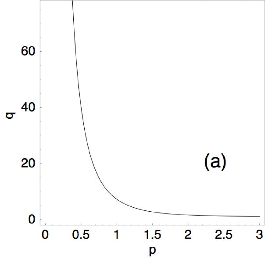
Figure 1: (a) TOKITA

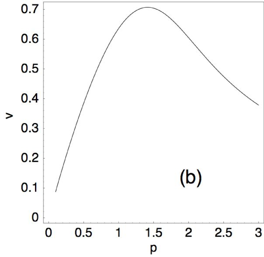
Figure 1: (b) TOKITA

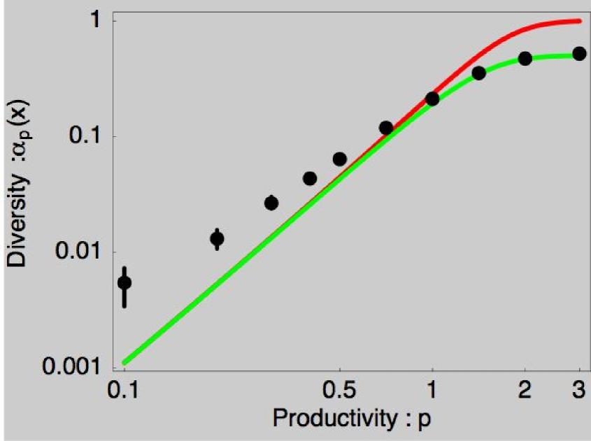
Figure 2: TOKITA

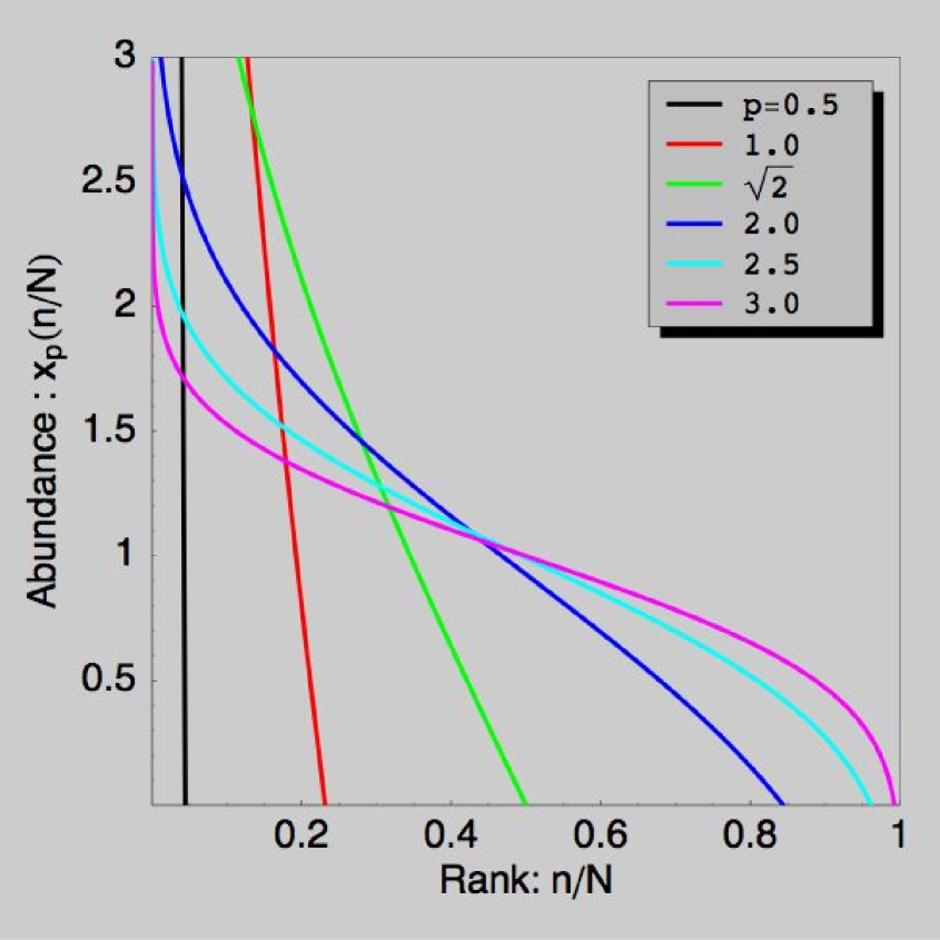
Figure 3: TOKITA

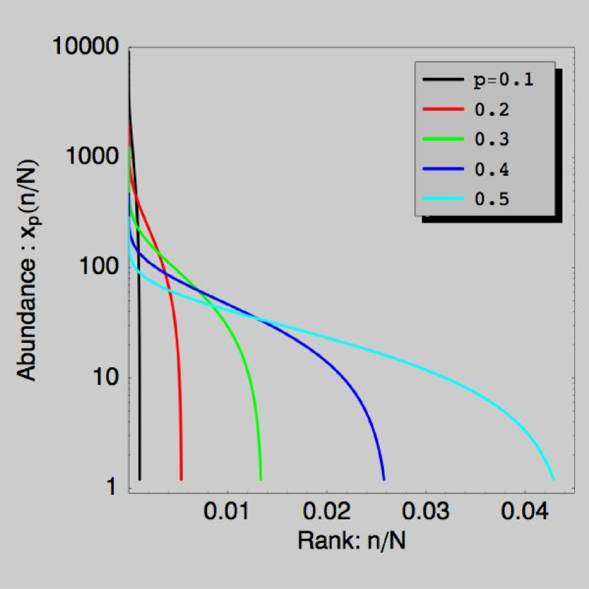
Figure 4: TOKITA

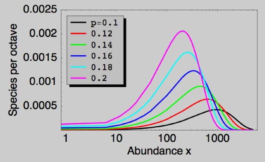
Figure 5: TOKITA

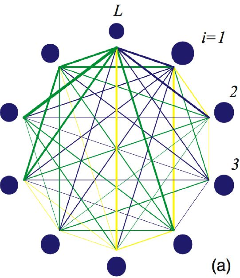
Figure 6: (a) TOKITA

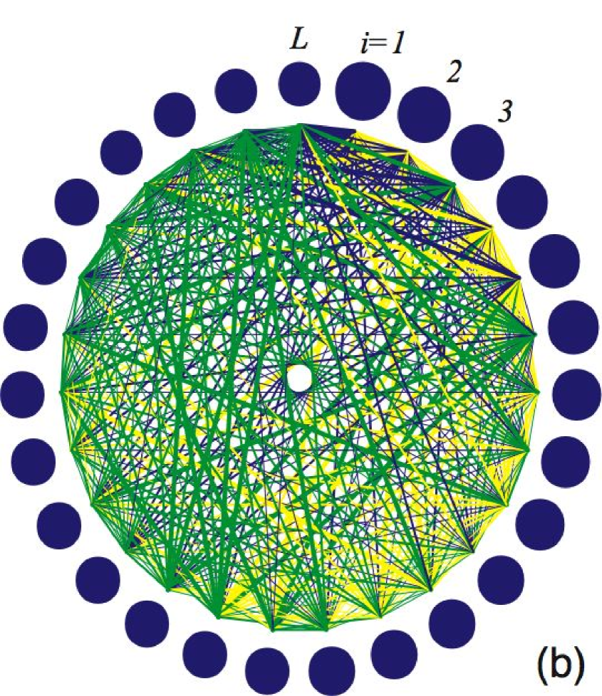
Figure 6: (b) TOKITA

References

• [1] N Martinez. Artifacts or attributes? effects of resolution on the little rock lake food web. Ecological Monographs, Vol. 61, pp. 367–392, 1991.
• [2] http://userwww.sfsu.edu/~webhead/lrl.html.
• [3] http://kr.expasy.org/cgi-bin/show_thumbnails.pl.
• [4] H. Jeong, S. Mason, A.-L. Barabási, and Z. N. Oltvai. Lethality and centrality in protein networks. Nature, Vol. 411, pp. 41–42, 2001.
• [5] http://www.nd.edu/~networks/gallery.htm.
• [6] A L Barabási. Linked. Perseus, 2002.
• [7] R Pastor-Satorras and A Vespignani. Epidemic dynamics and endemic states in complex networks. Phys. Rev. Lett., Vol. 63, p. 066117, 2001.
• [8] R. M. May. Unanswered questions in ecology. Phil. Trans. R. Soc. London, Vol. B 264, pp. 1951–1959, 1999.
• [9] I. Motomura. On the statistical treatment of communities. Zoological Magazine, Tokyo, Vol. 44, pp. 379–383, 1932.
• [10] A. S. Corbet, R. A. Fisher, and C. B. Williams. The relation between the number of species and the number of individuals in a random sample of an animal population. J. Anim. Ecol., Vol. 12, pp. 42–58, 1943.
• [11] R. H. MacArthur. On the relative abundance of bird species. Proc. Nat. Acad. Sci. USA, Vol. 43, pp. 293–295, 1957.
• [12] R. H. MacArthur. On the relative abundance of species. Am. Nat., Vol. 94, pp. 25–36, 1960.
• [13] F. W. Preston. The canonical distribution of commonness and rarity: Part 1. Ecology, Vol. 43, pp. 185–215, 1962.
• [14] F. W. Preston. The canonical distribution of commonness and rarity: Part 2. Ecology, Vol. 43, pp. 410–432, 1962.
• [15] R H Whittaker. Communities and Ecosystems. Macmillan, New York, 1970.
• [16] F A Bazzaz. Plant species diversity in oldfield successional ecosystems in southern illinois. Ecology, Vol. 56, pp. 485–488, 1975.
• [17] R. M. May. Patterns of species abundance and diversity, pp. 81–120. Belknap, Cambridge, 1975.
• [18] G Sugihara. Minimal community structure: an explanation of species abundance pattern. Am. Nat., Vol. 116, pp. 770–787, 1980.
• [19] S Nee, P H Harvey, and R M May. Lifting the veil on abundance patterns. Proc. R. Soc. Lond. B, Vol. 243, pp. 161–163, 1991.
• [20] M. Tokeshi. Species Coexistence. Blackwell, 1999.
• [21] S. P. Hubbell. The Unified Neutral Theory of Biodiversity and Biogeography. Princeton University Press, Princeton, 2001.
• [22] M Hall, K Christensen, S A di Collabiano, and H J Jensen. Time-dependent extinction rate and species abundance in a tangled-nature model of biological evolution. Phys. Rev. E, Vol. 66, p. 011904, 2002.
• [23] J Harte. Tail of death and resurrection. Nature, Vol. 424, pp. 1006–1007, 2003.
• [24] B. J. McGill. A test of the unified neutral theory of biodiversity. Nature, Vol. 422, pp. 881–885, 2003.
• [25] I. Volkov, J. R. Banavar, S. P. Hubbel., and A. Maritan. Neutral theory and relative species abundance in ecology. Nature, Vol. 424, pp. 1035–1037, 2003.
• [26] S Pigolotti, A Flammini, and A Maritan. Stochastic model for the species abundance problem in an ecological community. Phys. Rev. E, Vol. 70, p. 011916, 2004.
• [27] R S Etienne and H Olff. A novel genealogical approach to neutral biodiversity theory. Ecol. Lett., Vol. 7, pp. 170–175, 2004.
• [28] J Chave. Neutral theory and community ecology. Ecol. Lett., Vol. 7, pp. 241–253, 2004.
• [29] J Harte, E Conlisk, A Ostling, J L Green, and A B Smith. A theory of spatial structure in ecological communities at multiple spatial scales. Ecological Monographs, Vol. 75, pp. 179–197, 2005.
• [30] K. Tokita. Species abundance patterns in complex evolutionary dynamics. Phys. Rev. Lett., Vol. 93, pp. 178102–1$\sim$4, 2004.
• [31] J Hofbauer and K Sigmund. Evolutionary Games and Population Dynamics. Cambridge University Press, Cambridge, 1998.
• [32] R. H. MacArthur and R. Levins. The limiting similarity, convergence, and divergence of coexisting species. Am. Nat., Vol. 101, pp. 377–385, 1967.
• [33] R. M. May. Will a large complex system be stable? Nature, Vol. 238, pp. 413–414, 1972.
• [34] K. Tokita and A. Yasutomi. Emergence of a complex and stable ecosystem in replicator equations with extinction and mutation. Theor. Pop. Biol., Vol. 63, pp. 131–146, 2003.
• [35] M. R. Gardner and W. R. Ashby. Connectance of large dynamic (cybernetic) systems - critical values for stability. Nature, Vol. 228, p. 784, 1970.
• [36] K. Tokita and A. Yasutomi. Mass extinction in a dynamical system of evolution with variable dimension. Phys. Rev. E, Vol. 60, pp. 842–847, 1999.
• [37] M. Mezard, G. Parisi, and A. Virasoro. Spin Glass Theory and Beyond. World Scientific, Singapore, 1987.
• [38] S. Diederich and M. Opper. Replicators with random interactions: A solvable model. Phys. Rev. A, Vol. 39, pp. 4333–4336, 1989.
• [39] P. Biscari and G. Parisi. Replica symmetry breaking in the random replicant model. J. Phys. A: Math. Gen., Vol. 28, pp. 4697–4708, 1995.
• [40] V. M. de Oliveira and J. F. Fontanari. Random replicators with high-order interactions. Phys. Rev. Lett., Vol. 85, pp. 4984–4987, 2000.
• [41] V. M. de Oliveira and J. F. Fontanari. Extinctions in the random replicator model. Phys. Rev. E, Vol. 64, p. 051911, 2001.
• [42] V. M. de Oliveira and J. F. Fontanari. Complementarity and diversity in a soluble model ecosystem. Phys. Rev. Lett, Vol. 89, p. 148101, 2002.
• [43] H Nishimori. Statistical Physics of Spin Glasses and Information Processing : An Introduction. Oxford University Press, 2001.
• [44] R B Waide, et al. The relationship between productivity and species richness. Annu. Rev. Ecol. Syst., Vol. 30, pp. 257–300, 1999.
• [45] R. H. MacArthur and E. O. Wilson. Island Biogeography. Princeton University Press, Princeton, 1967.
• [46] M L Rosenzweig. Species Diversity in Space and Time. Cambridge Univ. Press, Cambridge, 1995.
• [47] D Tilman and S Pacala. Species Diversity in Ecological Communities: Historical and Geographical Perspectives, pp. 13–25. Univ. Chicago Press, New York, 1993.
• [48] W. J. Blake, M. Kærn, C. R. Cantor, and J. J. Collins. Noise in eukaryotic gene expression. Nature, Vol. 422, pp. 633–637, 2003.
• [49] K Kaneko. Recursiveness, switching, and fluctuations in a replicating catalytic networks. Phys. Rev. E, Vol. 68, p. 031909, 2003.
• [50] K. Sato, Y. Ito, T. Yomo, and K. Kaneko. On the relation between fluctuation and response in biological systems. Proc. Natl. Acad. Sci. USA, Vol. 100, pp. 14086–14090, 2003.