Schwinger Boson Formulation and Solution of the Crow-Kimura and Eigen Models of Quasispecies Theory

Abstract

We express the Crow-Kimura and Eigen models of quasispecies theory in a functional integral representation. We formulate the spin coherent state functional integrals using the Schwinger Boson method. In this formulation, we are able to deduce the long-time behavior of these models for arbitrary replication and degradation functions. We discuss the phase transitions that occur in these models as a function of mutation rate. We derive for these models the leading order corrections to the infinite genome length limit.

1 Introduction

The quasispecies models of Eigen ei71 and Crow-Kimura ck70 are among the simplest that capture basic aspects of mutation and evolutionary selection in large, homogeneous populations of viruses. These models are a favorite entry point for physicists to evolutionary biology, due to the phase transitions that they exhibit and their mathematical simplicity Krug .

While the models were originally defined in the continuous time limit, the first connections to statistical mechanics were made to the discrete-time versions of these models. In particular, the discrete-time Eigen model, which entails the additional assumption of allowing only a single mutation at one point in time in addition to discretization of time, was shown to be equivalent to a particular type of Ising model Leuthausser . A distinction between the bulk magnetization and the observable, surface, magnetization was discovered in the discrete-time Eigen model Tarazona , and an analogy to the surface wetting phenomenon in condensed matter was made. Magnetization is a now-standard term in the physical quasispecies field for average composition. That is, the magnetization at site $j$ on the genome is the average composition of the base at that site, averaged over all sequences in the population. A functional integral representation of the discrete-time Eigen model was introduced through use of functional delta functions Peliti2002 . With this representation, solution of this particular model was possible for viral replication rates that depend in an arbitrary way on distance from a single point in genome space. The closely related Crow-Kimura, or parallel or para-muse, continuous-time model was formulated as a quantum spin Hamiltonian in bb97 ; bb98 . It was formulated as a functional integral and solved for viral replication rates that depend in an arbitrary way on distance from a single point in genome space in sh04a ; sh04b ; sh04c . The discrete-time Eigen model in a sense interpolates between the continuous-time Eigen model and the Crow-Kimura model, because its limit as the time step becomes small is the Crow-Kimura model rather than the Eigen model. What distinguishes the continuous-time Eigen model from the other models is the possibility of multiple mutation events in an infinitesimal time step Krug .

In this manuscript we seek to provide a detailed derivation for a functional integral representation of the continuous-time parallel and Eigen models of quasispecies theory. These representations are used to find exact solutions of these continuous-time quasispecies theories in the limit of large genomes. These results are used to exhibit the phase transitions that occur in these models as a function of mutation rate. The coherent states formalism that we introduce allows for the first time the expression of the full time-dependent probability distribution in sequence space of these quasispecies theories as a function of arbitrary initial and final conditions. In addition, we use the functional integral expressions to obtain for the first time the $O(1/N)$ corrections to the mean replication rates in these models. Finally, we also use the functional integral expressions to find for the first time the $O(1/\sqrt{N})$ width of the virus populations around the most probable genomes in sequence space.

The rest of the manuscript is organized as follows. In Section 2 we map the continuous-time parallel model onto a spin coherent state path integral using the Schwinger Boson method. We evaluate the theory for a general replication rate. We find the corrections to the infinite genome limit. In Section 3 we map the continuous-time Eigen model onto a functional integral, again using the Schwinger Boson method. While the functional integral appears more singular than in the parallel case, due to the presence of multiple mutations at a single time step in this model, we also solve this model for a general replication rate. We also find the corrections to the infinite genome limit. We discuss the width of the virus population in genome space in the large $N$ limit and correlations in the field theory in Section 4. We also find the expression for the full time-dependent probability distribution as it depends on initial and final conditions. We conclude in Section 5. Much of the detailed derivations are included in Appendices.

2 Spin coherent state representation of the parallel model

2.1 The parallel model

In the parallel model, the probability distribution of viruses in the space of all possible viral genomes is considered. For simplicity, it is assumed that the genome can be written as a sequence of $N$ binary digits, or spins: $s_{n}^{i}=\pm 1$, $1\leq n\leq N$. Distances in the genome space are calculated by the Hamming measure: $d_{ij}=(N-\sum_{n}s_{n}^{i}s_{n}^{j})/2$. The probability for a virus to be in a given genome state, $p_{i}$, $1\leq i\leq 2^{N}$, satisfies the parallel model differential equation

$$\frac{{dp}_{i}}{dt}={p_{i}}(r_{i}-{\sum}_{j=1}^{2^{N}}r_{j}p_{j})+{\sum}_{j=1}^{2^{N}}\mu_{ij}p_{j}\ .$$ (1)

Here $r_{i}$ is the number of offspring per unit period of time, or replication rate, and $\mu_{ij}=\mu\Delta(d_{ij}-1)-N\mu\Delta(d_{ij})$ is the mutation rate to move from sequence $s_{i}$ to sequence $s_{j}$ per unit period of time. Here $\Delta(n)$ is the Kronecker delta. The non-linear term in Eq. (1) serves simply to enforce the conservation of probability, $\sum_{i}p_{i}=1$. We can express the differential equation in a simpler, linear form

$$\frac{{dq}_{i}}{dt}=r_{i}q_{i}+{\sum}_{j=1}^{2^{N}}\mu_{ij}q_{j}$$ (2)

with the transformation $p_{i}(t)=q_{i}(t)/\sum_{j}q_{j}(t)$. The explicit form of the replication rate is $r_{i}=Nf(u)$, where $u=(1/N)\sum_{n}s^{i}_{n}$.

2.2 The parallel model in operator form

Motivated by the observation bb97 that the parallel dynamics in Eq. (2) is equivalent to quantum dynamics in imaginary time, we express the model in an operator form. We define two kinds of creation and annihilation operators: $\hat{a}_{\alpha}(j),\hat{a}^{\dagger}_{\alpha}(j)$, $\alpha=1,2$ and $j=1,\ldots,N$. These operators obey the commutation relations

$$\left[\hat{a}_{\alpha}(i),\hat{a}^{\dagger}_{\beta}(j)\right] = \delta_{\alpha\beta}\delta_{ij}$$

$$\left[\hat{a}_{\alpha}(i),\hat{a}_{\beta}(j)\right] = 0$$

$$\left[\hat{a}^{\dagger}_{\alpha}(i),\hat{a}^{\dagger}_{\beta}(j)\right] = 0$$ (3)

These operators create either a spin-up state for $\alpha=1$ or a spin-down state for $\alpha=2$ at position $j$ in the genome. While it might see more natural to introduce a single set of creation and annihilation operators to define whether the spin at position $j$ is up or down, this approach leads to a non-Gaussian field theory even for a vanishing replication rate function. Use of two sets of creation and annihilation operators leads to a Gaussian field theory, with non-quadratic terms stemming from the replication rate function. We find this second form of the theory more convenient for calculation. This second form, moreover, can be extended to the case where the sequence alphabet is larger than binary. Since the state is one and only one of the possible letters at position $j$, spin-up or spin-down in the binary alphabet case considered here, we will enforce the constraint that

$$\sum_{\alpha}\hat{a}^{\dagger}_{\alpha}(j)\hat{a}_{\alpha}(j)=1$$ (4)

for all $j$. Thus, the state at site $j$ is either

$$|1,0\rangle=[\hat{a}^{\dagger}_{1}(j)]^{1}[\hat{a}^{\dagger}_{2}(j)]^{0}|0,0\rangle{\rm~{}or~{}}|0,1\rangle=[\hat{a}^{\dagger}_{1}(j)]^{0}[\hat{a}^{\dagger}_{2}(j)]^{1}|0,0\rangle$$ (5)

Defining $n_{j}^{i}$ to be the power on $\hat{a}^{\dagger}_{1}(j)$ for spin state $i$, we can rewrite the parallel model dynamics as

$$\frac{d}{dt}P(\{n^{i}_{j}\}) = r_{i}(\{n^{i}_{j}\})P(\{n^{i}_{j}\})+\mu\sum_{j=1}^{N}\bigg{[}(1-n_{j}^{i})P(\{\ldots,n_{j}^{i}+1,\ldots\})$$ (6)

$$+n_{j}^{i}P(\{\ldots,n^{i}_{j}-1,\ldots\})-P(\{n^{i}_{j}\})\bigg{]}$$

We introduce the state vector

$$|\psi\rangle=\sum_{i=1}^{2^{N}}P(\{n^{i}\})|\{n^{i}\}\rangle$$ (7)

which satisfies the differential equation

$$\frac{d}{dt}|\psi\rangle=\sum_{i=1}^{2^{N}}\frac{dP(\{n^{i}\})}{dt}|\{n^{i}\}\rangle$$ (8)

We now write this Eq. (8) in operator form. First, we introduce vector notation for the creation and annihilation operators: $\hat{\vec{a}}(j)=(\hat{a}_{1}(j),\hat{a}_{2}(j))$ and $\hat{\vec{a}}^{\dagger}(j)=(\hat{a}_{1}^{\dagger}(j),\hat{a}_{2}^{\dagger}(j))$. Then we introduce operators

$$T_{i}(j) = \hat{\vec{a}}^{\dagger}(j)\sigma_{i}\hat{\vec{a}}(j)$$

$$T_{0} = \hat{\vec{a}}^{\dagger}(j)\cdot\hat{\vec{a}}(j)$$ (9)

with spin matrices

$$\sigma_{1}=\left(\begin{array}[]{cc}0&1\\ 1&0\end{array}\right),~{}~{}\sigma_{2}=\left(\begin{array}[]{cc}0&-1\\ 1&0\end{array}\right),~{}~{}\sigma_{3}=\left(\begin{array}[]{cc}1&0\\ 0&-1\end{array}\right)$$ (16)

Then the dynamics of Eq. (8) can be written as

$$\frac{d}{dt}|\psi\rangle=-\hat{H}|\psi\rangle$$ (17)

with

$$-\hat{H}=Nf\left[\sum_{j=1}^{N}T_{3}(j)/N\right]+\mu\sum_{j=1}^{N}[T_{1}(j)-T_{0}(j)]$$ (18)

2.3 The field theoretic representation of the parallel model

We convert this operator form of the parallel model into a functional integral by using coherent states. We define a spin coherent state by

$$|\vec{z}(j)\rangle = e^{\hat{\vec{a}}^{\dagger}(j)\cdot\vec{z}(j)-\vec{z}^{*}(j)\cdot\hat{\vec{a}}(j)}|(0,0)(j)\rangle$$ (19)

$$= e^{-\frac{1}{2}\vec{z}^{*}(j)\cdot\vec{z}(j)}\sum_{n,m=0}^{\infty}\frac{[z_{1}(j)]^{n}[z_{2}(j)]^{m}}{\sqrt{n!m!}}|(n,m)(j)\rangle$$

These coherent states satisfy a completeness relation

$$I=\int\prod_{j=1}^{N}\frac{d\vec{z}^{*}(j)d\vec{z}(j)}{\pi^{2}}|\{|\vec{z}\}\rangle\langle\{|\vec{z}\}|$$ (20)

The overlap of coherent states satisfies

$$\langle\vec{z}^{\prime}(j)|\vec{z}(j)\rangle=e^{-\frac{1}{2}\{{\vec{z}^{\prime}}^{*}(j)\cdot[\vec{z}^{\prime}(j)-\vec{z}(j)]-[\vec{z}^{\prime*}(j)-\vec{z}^{*}(j)]\cdot\vec{z}(j)\}}$$ (21)

Equation (17) enforces constraint (4) if the initial conditions obey the constraint. To project arbitrary initial conditions onto this constraint, we use the operator

$$\hat{P} = \prod_{j=1}^{N}\hat{P}(j)=\prod_{j=1}^{N}\Delta[\hat{\vec{a}}^{\dagger}(j)\cdot\hat{\vec{a}}(j)-1]$$ (22)

$$= \int_{0}^{2\pi}\prod_{j=1}^{N}\frac{d\lambda_{j}}{2\pi}e^{i\lambda_{j}[\hat{\vec{a}}^{\dagger}(j)\cdot\hat{\vec{a}}(j)-1]}$$

The probability to be in a given final state at time $t$ is

$$P(\{\vec{n}\},t)=\sum_{\{\vec{n}_{0}\}}\langle\{\vec{n}\}|e^{-\hat{H}t}|\{\vec{n}_{0}\}\rangle P(\{\vec{n}_{0}\})$$ (23)

Using the coherent states identity in a Trotter factorization, we find

$$P(\{\vec{n}\},t) = \sum_{\{\vec{n}_{0}\}}\lim_{M\to\infty}\langle\{\vec{n}\}|\int\left[\prod_{j=1}^{N}\frac{d\vec{z}^{*}_{M}(j)d\vec{z}_{M}(j)}{\pi^{2}}\right]|\{\vec{z}_{M}\}\rangle\langle\{\vec{z}_{M}\}|e^{-\epsilon\hat{H}}$$ (24)

$$\times\int\left[\prod_{j=1}^{N}\frac{d\vec{z}^{*}_{M-1}(j)d\vec{z}_{M-1}(j)}{\pi^{2}}\right]|\{\vec{z}_{M-1}\}\rangle\langle\{\vec{z}_{M-1}\}|e^{-\epsilon\hat{H}}$$

$$\vdots$$

$$\int\left[\prod_{j=1}^{N}\frac{d\vec{z}^{*}_{1}(j)d\vec{z}_{1}(j)}{\pi^{2}}\right]|\{\vec{z}_{1}\}\rangle\langle\{\vec{z}_{1}\}|e^{-\epsilon\hat{H}}$$

$$\times\int\left[\prod_{j=1}^{N}\frac{d\vec{z}^{*}_{0}(j)d\vec{z}_{0}(j)}{\pi^{2}}\right]e^{-\epsilon\hat{H}}\hat{P}|\{\vec{z}_{0}\}\rangle\langle\{\vec{z}_{0}\}|\{\vec{n}_{0}\}\rangle P(\{\vec{n}_{0}\})$$

$$= \lim_{M\to\infty}\int[{\cal D}\vec{z}^{*}{\cal D}\vec{z}]\langle\{\vec{n}\}|\{\vec{z}_{M}\}\rangle\left(\sum_{\{\vec{n}_{0}\}}\langle\{\vec{z}_{0}\}|\{\vec{n}_{0}\}\rangle P(\{\vec{n}_{0}\})\right)$$

$$\times\prod_{k=2}^{M}\langle\{|\vec{z}_{k}\}|e^{-\epsilon\hat{H}}|\{\vec{z}_{k-1}\}\rangle\langle\{\vec{z}_{1}\}|e^{-\epsilon\hat{H}}\hat{P}|\{\vec{z}_{0}\}\rangle$$

For initial conditions that satisfy constraint (4)

$$\langle\{\vec{n}\}|\{\vec{z}_{M}\}\rangle = \prod_{j}e^{-\frac{1}{2}\vec{z}^{*}_{M}(j)\cdot\vec{z}_{M}(j)}\vec{n}(j)\cdot\vec{z}_{M}(j)$$

$$\langle\{\vec{z}_{0}\}|\{\vec{n}_{0}\}\rangle = \prod_{j}e^{-\frac{1}{2}\vec{z}^{*}_{0}(j)\cdot\vec{z}_{0}(j)}\vec{z}_{0}^{*}(j)\cdot\vec{n}_{0}(j)$$ (25)

Conversely, if the projection operator is needed for arbitrary initial conditions, we note

$$\hat{P}|\vec{z}_{0}(j)\rangle = \int_{0}^{2\pi}\prod_{j=1}^{N}\frac{d\lambda_{j}}{2\pi}e^{-i\lambda_{j}}e^{i\lambda_{j}\hat{\vec{a}}^{\dagger}(j)\cdot\hat{\vec{a}}(j)}|\vec{z}(j)\rangle$$ (26)

$$= \int_{0}^{2\pi}\prod_{j=1}^{N}\frac{d\lambda_{j}}{2\pi}e^{-i\lambda_{j}}|(e^{i\lambda_{j}}\vec{z})(j)\rangle$$

For initial conditions that satisfy constraint (4), we may remove the projection operator to find

$$P(\{\vec{n}\},t) = \lim_{M\to\infty}\int[{\cal D}\vec{z}^{*}{\cal D}\vec{z}]\sum_{\{\vec{n}_{0}\}}P(\{\vec{n}_{0}\})\prod_{j=1}^{N}\vec{n}(j)\cdot\vec{z}_{M}(j)\vec{z}_{0}^{*}(j)\cdot\vec{n}_{0}(j)$$ (27)

$$\times e^{-\frac{1}{2}\vec{z}^{*}_{M}(j)\cdot\vec{z}_{M}(j)}e^{-\frac{1}{2}\vec{z}^{*}_{0}(j)\cdot\vec{z}_{0}(j)}$$

$$\times\prod_{k=1}^{M}e^{-\frac{1}{2}\{{\vec{z}}_{k}^{*}(j)\cdot[\vec{z}_{k}(j)-\vec{z}_{k-1}(j)]-[(\vec{z})^{*}_{k}(j)-\vec{z}^{*}_{k-1}(j)]\cdot\vec{z}_{k-1}(j)\}}$$

$$\times e^{\epsilon Nf\left[\sum_{j=1}^{N}{\vec{z}}^{*}_{k}(j)\sigma_{3}{\vec{z}}_{k-1}(j)/N\right]+\epsilon\Delta f({\vec{z}}^{*}_{k},{\vec{z}}_{k-1})}$$

$$\times e^{\epsilon\mu\sum_{j=1}^{N}[{\vec{z}}^{*}_{k}(j)\sigma_{1}{\vec{z}}_{k-1}(j)-1]}$$

$$= \lim_{M\to\infty}\int[{\cal D}\vec{z}^{*}{\cal D}\vec{z}]\sum_{\{\vec{n}_{0}\}}P(\{\vec{n}_{0}\})$$

$$\times\prod_{j=1}^{N}\vec{n}(j)\cdot\vec{z}_{M}(j)~{}\vec{z}_{0}^{*}(j)\cdot\vec{n}_{0}(j)~{}e^{-S[\vec{z}^{*},\vec{z}]}$$

where

$$S[\vec{z}^{*},\vec{z}] = \vec{z}^{*}_{0}(j)\cdot\vec{z}_{0}(j)+\sum_{k=1}^{M}{\vec{z}}_{k}^{*}(j)\cdot[\vec{z}_{k}(j)-\vec{z}_{k-1}(j)]$$ (28)

$$-\epsilon\sum_{k=1}^{M}\bigg{\{}Nf\left[\sum_{j=1}^{N}{\vec{z}}^{*}_{k}(j)\sigma_{3}{\vec{z}}_{k-1}(j)/N\right]+\Delta f({\vec{z}}^{*}_{k},{\vec{z}}_{k-1})$$

$$+\mu\sum_{j=1}^{N}[{\vec{z}}^{*}_{k}(j)\sigma_{1}{\vec{z}}_{k-1}(j)-1]\bigg{\}}$$

where $\epsilon=t/M$. To evaluate the expression involving $Nf[\{\hat{\vec{a}}^{\dagger}\},\{\hat{\vec{a}}\}]$, we use normal ordering. We define

$$Nf[\{\hat{\vec{a}}^{\dagger}\},\{\hat{\vec{a}}\}]=N:f[\{\hat{\vec{a}}^{\dagger}\},\{\hat{\vec{a}}\}]:+\Delta f[\{\hat{\vec{a}}^{\dagger}\},\{\hat{\vec{a}}\}]$$ (29)

where the notation $:(\cdot):$ means in the operator expression for $(\cdot)$, place all of the $\{\hat{\vec{a}}^{\dagger}\}$ to the left of the $\{\hat{\vec{a}}\}$. The additional terms that this operator commutation generates are collected in $\Delta f$. We note that N $:f:$ is $O(N)$, whereas $\Delta f$ is $O(1)$. For example, for the quadratic replication rate $f(u)=\frac{\gamma}{2}u^{2}$, we find

$$Nf[\frac{1}{N}\sum_{j=1}^{N}\hat{\vec{a}}^{\dagger}(j)\sigma_{3}\hat{\vec{a}}(j)] = \frac{N\gamma}{2}[\frac{1}{N}\sum_{j=1}^{N}\hat{\vec{a}}^{\dagger}(j)\sigma_{3}\hat{\vec{a}}(j)]^{2}$$ (30)

$$= \frac{\gamma}{2N}\sum_{i,j=1}^{N}\hat{\vec{a}}^{\dagger}(i)\sigma_{3}(i)\hat{\vec{a}}(i)\hat{\vec{a}}^{\dagger}(j)\sigma_{3}(j)\hat{\vec{a}}(j)$$

$$= \frac{\gamma}{2N}\sum_{i,j=1}^{N}\hat{\vec{a}}^{\dagger}(i)\sigma_{3}(i)[\hat{\vec{a}}^{\dagger}(j)\hat{\vec{a}}(i)+\delta_{ij}]\sigma_{3}(j)\hat{\vec{a}}(j)$$

$$= \frac{N\gamma}{2}:[\frac{1}{N}\sum_{j=1}^{N}\hat{\vec{a}}^{\dagger}(j)\sigma_{3}\hat{\vec{a}}(j)]^{2}:+\frac{\gamma}{2N}\sum_{j=1}^{N}\hat{\vec{a}}^{\dagger}(j)\cdot\hat{\vec{a}}(j)$$

$$= N:f(\sum_{j=1}^{N}\hat{\vec{a}}^{\dagger}(j)\sigma_{3}\hat{\vec{a}}(j)/N):+\frac{\gamma}{2}$$

so that $\Delta f=\gamma/2$ in this quadratic case. By induction, we can show that the general form of the commutation term is

$$\Delta f=\frac{1}{2}\frac{d^{2}f(\xi)}{d\xi^{2}}$$ (31)

In the continuous limit, the probability at time $t$ becomes

$$P(\{\vec{n}\},t) = \int[{\cal D}\vec{z}^{*}{\cal D}\vec{z}]\sum_{\{\vec{n}_{0}\}}P(\{\vec{n}_{0}\})\prod_{j=1}^{N}\vec{n}_{j}(t)\cdot\vec{z}_{j}(t)~{}\vec{z}_{j}^{*}(0)\cdot\vec{n}_{j}(0)~{}e^{-S[\vec{z}^{*},\vec{z}]}$$

where we have switched the subscripts and arguments of the variables and where

$$S[\vec{z}^{*},\vec{z}] = \int_{0}^{t}dt^{\prime}\sum_{j=1}^{N}\vec{z}_{j}^{*}(t^{\prime})[\partial_{t}-\mu\sigma_{1}(j)+\delta(t)]\vec{z}_{j}(t^{\prime})+\mu Nt$$ (33)

$$-N\int_{0}^{t}dt^{\prime}f\left[\sum_{j=1}^{N}{\vec{z}}^{*}_{j}(t^{\prime})\sigma_{3}{\vec{z}}_{j}(t^{\prime})/N\right]$$

$$-\int_{0}^{t}dt^{\prime}\Delta f\left[\{{\vec{z}}^{*}(t^{\prime})\},\{\vec{z}(t^{\prime})\}\right]$$

At long times, we find that $e^{-\hat{H}t}|\{{\bf n}_{0}\}\rangle\sim e^{f_{m}t}|{\bf n}^{*}\rangle$ by the Frobenius-Perrone Theorem Bapat , independent of initial conditions, where $f_{m}$ is the unique largest eigenvalue of $\hat{H}$, and $|{\bf n}^{*}\rangle$ is the corresponding eigenvector. To evaluate this eigenvalue, we consider the matrix trace. We, furthermore, incorporate the projection operator by the twisted boundary condition $\vec{z}_{0}(j)=e^{i\lambda_{j}}\vec{z}_{M}(j)$ arising from Eq. (26). We find

$${Z} = {\rm Tr}e^{-t\hat{H}}\hat{P}$$ (34)

$$= \int_{0}^{2\pi}\left[\prod_{j=1}^{N}\frac{d\lambda_{j}}{2\pi}e^{-i\lambda_{j}}\right]\lim_{M\to\infty}\int\left[\prod_{k=1}^{M}\prod_{j=1}^{N}\frac{d\vec{z}_{k}^{*}(j)d\vec{z}_{k}(j)}{\pi^{2}}\right]e^{-S[\vec{z}^{*},\vec{z}]}$$

where

$$e^{-S[\vec{z}^{*},\vec{z}]}=\prod_{k=1}^{M}\langle\{\vec{z}_{k}\}|e^{-\epsilon\hat{H}}|\{\vec{z}_{k-1}\}\rangle$$ (35)

with boundary condition $\vec{z}_{0}(j)=e^{i\lambda_{j}}\vec{z}_{M}(j)$. The action is Eq. (28), without the initial $\vec{z}^{*}_{0}(j)\cdot\vec{z}_{0}(j)$ term. Since the replication rate depends only on the total magnetization, the expression for $Z$ can be simplified. In particular, we introduce $\xi_{k}=\frac{1}{N}\sum_{j=1}^{N}{\vec{z}}^{*}_{k}(j)\sigma_{3}{\vec{z}}_{k-1}(j)$ to find, as discussed in Appendix A, that the partition function becomes

$$Z=\int[{\cal D}\bar{\xi}{\cal D}\xi]e^{-S[\bar{\xi},\xi]}$$ (36)

where

$$S[\bar{\xi},\xi]=N\int_{0}^{t}dt^{\prime}\left\{-f[\xi(t^{\prime})]+\bar{\xi}(t^{\prime})\xi(t^{\prime})+\mu-\frac{1}{N}\Delta f\right\}-N\ln Q$$ (37)

and

$$Q={\rm Tr}\hat{T}e^{\int_{0}^{t}dt^{\prime}[\mu\sigma_{1}+\bar{\xi}(t^{\prime})\sigma_{3}]}$$ (38)

2.4 The large $N$ limit of the parallel model is a saddle point

The general expression of the parallel model partition function involves a functional integral. Using that $N$ is large, this functional integral can be evaluated by the saddle point method. We impose the saddle point condition to find

$$\left.\frac{\delta S}{\delta\bar{\xi}}\right|_{\bar{\xi}_{c},\xi_{c}} = 0=N\xi_{c}-N\frac{{\rm Tr}\hat{T}\sigma_{3}e^{\int_{0}^{t}dt^{\prime}[\mu\sigma_{1}+\bar{\xi}_{c}\sigma_{3}]}}{{\rm Tr}\hat{T}e^{\int_{0}^{t}dt^{\prime}[\mu\sigma_{1}+\bar{\xi}_{c}\sigma_{3}]}}$$

$$\left.\frac{\delta S}{\delta\xi}\right|_{\bar{\xi}_{c},\xi_{c}} = 0=-Nf^{\prime}(\xi_{c})+N\bar{\xi}_{c}$$ (39)

Evaluating the traces, we find

$$\bar{\xi}_{c} = f^{\prime}(\xi_{c})$$

$$\xi_{c} = \frac{\bar{\xi}_{c}}{[\mu^{2}+\bar{\xi}_{c}^{2}]^{1/2}}\tanh t[\mu^{2}+\bar{\xi}_{c}^{2}]^{1/2}$$ (40)

For large $t$ we can solve Eq. (40) for $\bar{\xi}_{c}$ to find

$$\bar{\xi}_{c}\sim\frac{\mu\xi_{c}}{\sqrt{1-\xi_{c}^{2}}}$$ (41)

and evaluate Eq. (109) to find

$$\ln Q\sim t\sqrt{\mu^{2}+\bar{\xi}_{c}^{2}}=t\frac{\mu}{\sqrt{1-\xi_{c}^{2}}}$$ (42)

Using Eqs. (41–42) in Eq. (37), we find that $\xi_{c}$ is the value which maximizes

$$\frac{\ln Z}{tN} = f[\xi_{c}]-\frac{\mu\xi_{c}^{2}}{\sqrt{1-\xi_{c}^{2}}}-\mu+\frac{\mu}{\sqrt{1-\xi_{c}^{2}}}+\frac{\Delta f}{N}$$ (43)

$$= f[\xi_{c}]+\mu\sqrt{1-\xi_{c}^{2}}-\mu+\frac{\Delta f}{N}$$

This expression is the saddle point evaluation of the parallel model partition function. It is valid for arbitrary replication rate functions $f$.

As an example, we calculate the error threshold for two different replication rate functions. For our first example, we take the case of $f(1)=A$ and $f=0$ otherwise. This case leads to the phase transition at $A/\mu=1$. For $A/\mu>1$ a finite fraction $p_{1}$ of the population is at $\xi_{c}=1$, whereas for $A/\mu<1$, all of the population is at $\xi_{c}=0$. The fraction of the population at $\xi_{c}=1$ is determined by the implicit equation $p_{1}f(1)+(1-p_{1})f(\xi\neq 1)=\left.\ln Z/(tN)\right|_{\xi_{c}}$, which gives $p_{1}=1-\mu/A$. For our second example, we consider the quadratic fitness $f(\xi)=k\xi^{2}/2$ bb97 . We find a phase transition at $k/\mu=1$, where the selected phase occurs for $k/\mu>1$ with an average magnetization given by $\xi_{c}=\pm\sqrt{1-(\mu/k)^{2}}$. The observable, surface magnetization, $u_{*}$, is given by the implicit expression $f(u_{*})=\left.\ln Z/(tN)\right|_{\xi_{c}}$ so that $u_{*}=\pm(1-\mu/k)$.

2.5 $O(1/N)$ corrections to the parallel model

We now evaluate the fluctuation corrections to this result. This procedure will determine the other $O(1/N)$ contributions to the mean replication rate per site, $(\ln Z)/(tN)$. We expand the action around the saddle point limit

$$S[\bar{\xi},\xi] = S(\bar{\xi}_{c},\xi_{c})+\frac{1}{2}\sum_{k,l=1}^{M}\bigg{[}\left.\frac{\partial^{2}S}{\partial\xi_{k}\partial\xi_{l}}\right|_{\bar{\xi}_{c},\xi_{c}}\delta\xi_{k}\delta\xi_{l}+2\left.\frac{\partial^{2}S}{\partial\xi_{k}\partial\bar{\xi}_{l}}\right|_{\bar{\xi}_{c},\xi_{c}}\delta\xi_{k}\delta\bar{\xi}_{l}$$ (44)

$$+\left.\frac{\partial^{2}S}{\partial\bar{\xi}_{k}\partial\bar{\xi}_{l}}\right|_{\bar{\xi}_{c},\xi_{c}}\delta\bar{\xi}_{k}\delta\bar{\xi}_{l}\bigg{]}$$

We find

$$\left.\frac{\partial^{2}S}{\partial\xi_{k}\partial\xi_{l}}\right|_{\bar{\xi}_{c},\xi_{c}} = -N\epsilon f^{\prime\prime}(\xi_{c})\delta_{kl}$$

$$\left.\frac{\partial^{2}S}{\partial\xi_{k}\partial\bar{\xi}_{l}}\right|_{\bar{\xi}_{c},\xi_{c}} = \epsilon N\delta_{kl}$$

$$\left.\frac{\partial^{2}S}{\partial\bar{\xi}_{k}\partial\bar{\xi}_{l}}\right|_{\bar{\xi}_{c},\xi_{c}} = -N\epsilon^{2}\frac{{\rm Tr}\sigma_{3}e^{\epsilon|l-k|(\mu\sigma_{1}+\bar{\xi}_{c}\sigma_{3})}\sigma_{3}e^{\epsilon(M-|l-k|)(\mu\sigma_{1}+\bar{\xi}_{c}\sigma_{3})}}{{\rm Tr}e^{\epsilon M(\mu\sigma_{1}+\bar{\xi}_{c}\sigma_{3})}}$$ (45)

$$+N\epsilon^{2}\left(\frac{{\rm Tr}\sigma_{3}e^{\epsilon M(\mu\sigma_{1}+\bar{\xi}_{c}\sigma_{3})}}{{\rm Tr}e^{\epsilon M(\mu\sigma_{1}+\bar{\xi}_{c}\sigma_{3})}}\right)^{2}$$

These terms, and the matrix trace, are evaluated in Appendix B. Solving the result of Eq. (123) for $\bar{\xi}_{c}$ in terms of $\xi_{c}$, we find

$$\frac{\ln Z}{tN} = f[\xi_{c}]+\mu\sqrt{1-\xi_{c}^{2}}-\mu+\frac{\Delta f}{N}-\frac{f^{\prime\prime}(\xi_{c})}{2N}$$ (46)

$$+\frac{1}{N}\frac{\mu}{\sqrt{1-\xi_{c}^{2}}}\left[1-\left[1-f^{\prime\prime}(\xi_{c})(1-\xi_{c}^{2})^{3/2}/\mu\right]^{1/2}\right]$$

Using Eq. (31) we find

$$\frac{\ln Z}{tN} = f[\xi_{c}]+\mu\sqrt{1-\xi_{c}^{2}}-\mu$$ (47)

$$+\frac{1}{N}\frac{\mu}{\sqrt{1-\xi_{c}^{2}}}\left[1-\left[1-f^{\prime\prime}(\xi_{c})(1-\xi_{c}^{2})^{3/2}/\mu\right]^{1/2}\right]$$

This is the expression of the parallel model partition function accurate to $O(1/N^{2})$. The expression is accurate for arbitrary smooth replication rate functions $f$. Shown in Figure 1 is the comparison between this analytical result and a numerical calculation following the algorithm in bb97 .

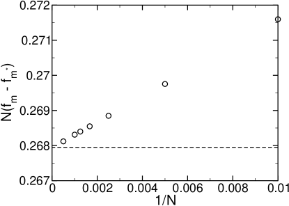
Figure 1: The $O(1/N)$ shift in the free energy is shown (circles). Also shown is the prediction from Eq. (47) (dashed line). We use $f(m)=km^{2}/2$ with $k/\mu=2$ and $\mu=1$.

3 Spin coherent state representation of the Eigen model

3.1 The Eigen model

In the Eigen model, the probability distribution of viruses in the space of all possible viral genomes is considered, as in the parallel model. However, when a virus replication event occurs, the virus copies its genome, making mutations at a rate of $1-q$ per base during the replication. The probability distribution in genome space satisfies

$$\frac{dp_{i}}{dt}=\sum_{j=1}^{2^{N}}\left[B_{ij}r_{j}-\delta_{ij}D_{j}\right]p_{j}-p_{i}\left[\sum_{j=1}^{2^{N}}(r_{j}-D_{j})p_{j}\right]\ .$$ (48)

Here the transition rates are given by $B_{ij}=q^{N-d(i,j)}(1-q)^{d(i,j)}$. We define the parameter $\mu=N(1-q)/q$ to characterize the per genome replication rate. We take $\mu=O(1)$. We define $q^{N}=e^{-\mu_{1}}$ and note that in the large $N$ limit, $\mu_{1}\to\mu$. As with the parallel model, the non-linear terms simply enforce conservation of probability, and it suffices to consider the linear terms only

$$\frac{dq_{i}}{dt}=\sum_{j=1}^{2^{N}}\left[B_{ij}r_{j}-\delta_{ij}D_{i}\right]q_{j}$$ (49)

As with the replication rate, the degradation rate is defined by $D_{i}=Nd(u)$, where $u=(1/N)\sum_{n}s^{i}_{n}$.

3.2 The Eigen model in operator form

Using the creation and annihilation operator formalism, the dynamics can be again written in the form of Eq. (17), with

$$-\hat{H} = \prod_{j=1}^{N}[qT_{0}(j)+(1-q)T_{1}(j)]Nf\left[\sum_{k=1}^{N}T_{3}(k)/N\right]-Nd\left[\sum_{j=1}^{N}T_{3}(j)/N\right]$$ (50)

$$= Ne^{-\mu_{1}}\prod_{j=1}^{N}[1+\frac{\mu}{N}T_{1}(j)]f\left[\sum_{k=1}^{N}T_{3}(k)/N\right]-Nd\left[\sum_{j=1}^{N}T_{3}(j)/N\right]$$

$$\sim Ne^{-\mu_{1}}e^{\sum_{j=1}^{N}\mu T_{1}(j)/N}f\left[\sum_{k=1}^{N}T_{3}(k)/N\right]-Nd\left[\sum_{j=1}^{N}T_{3}(j)/N\right]$$

where the last expression is valid for large $N$. Corrections to this expression will come from $\mu_{1}\neq\mu$, the exponential not being exactly equal to the product, as well as normal ordering terms. We will address these corrections later.

3.3 The field theoretic representation of the Eigen model

We introduce the Schwinger spin coherent states. We consider the normal ordered form of the Hamiltonian, and first consider the expression $:\hat{H}:$. We will consider the commutator terms later. We find $P(\{\vec{n}\},t)$ can be expressed as in Eq. (27) and the partition function $Z$ can be expressed as in Eq. (34) with

$$S[\vec{z}^{*},\vec{z}] = \prod_{k=1}^{M}\langle\{\vec{z}_{k}\}|e^{-\epsilon:\hat{H}:}|\{\vec{z}_{k-1}\}\rangle$$ (51)

$$= \vec{z}^{*}_{0}(j)\cdot\vec{z}_{0}(j)+\sum_{k=1}^{M}{\vec{z}}_{k}^{*}(j)\cdot[\vec{z}_{k}(j)-\vec{z}_{k-1}(j)]$$

$$+\epsilon N\sum_{k=1}^{M}\bigg{\{}e^{-\mu_{1}}e^{\mu\sum_{j=1}^{N}{\vec{z}}_{k}^{*}(j)\sigma_{1}\vec{z}_{k-1}(j)/N}f\left[\sum_{j=1}^{N}{\vec{z}}^{*}_{k}(j)\sigma_{3}{\vec{z}}_{k-1}(j)/N\right]$$

$$-d\left[\sum_{j=1}^{N}{\vec{z}}^{*}_{k}(j)\sigma_{3}{\vec{z}}_{k-1}(j)/N\right]\bigg{\}}$$

For the partition function case, we have the boundary condition $\vec{z}_{0}(j)=e^{i\lambda_{j}}\vec{z}_{M}(j)$. We introduce $\xi_{k}=\frac{1}{N}\sum_{j=1}^{N}{\vec{z}}^{*}_{k}(j)\sigma_{3}{\vec{z}}_{k-1}(j)$ and $\eta_{k}=\frac{1}{N}\sum_{j=1}^{N}{\vec{z}}^{*}_{k}(j)\sigma_{1}{\vec{z}}_{k-1}(j)$ to find, as discussed in Appendix C, that the partition function becomes

$$Z=\int[{\cal D}\bar{\xi}{\cal D}\xi][{\cal D}\bar{\eta}{\cal D}\eta]e^{-S[\bar{\xi},\xi,\bar{\eta},\eta]}$$ (52)

where

$$S[\bar{\xi},\xi,\bar{\eta},\eta] = N\int_{0}^{t}dt^{\prime}\left\{-e^{-\mu_{1}}e^{\mu\eta(t^{\prime})}f[\xi(t^{\prime})]+d[\xi(t^{\prime})]+\bar{\xi}(t^{\prime})\xi(t^{\prime})+\bar{\eta}(t^{\prime})\eta(t^{\prime})\right\}$$ (53)

$$-N\ln Q$$

3.4 The large $N$ limit of the Eigen model is a saddle point

The partition function of the Eigen model is represented as a functional integral. In the limit of large $N$, this integral can be evaluated by the saddle point method. The saddle point conditions are

$$\left.\frac{\delta S}{\delta\bar{\xi}}\right|_{\bar{\xi}_{c},\xi_{c},\bar{\eta}_{c},\eta_{c}} = 0=N\xi_{c}-N\frac{{\rm Tr}\hat{T}\sigma_{3}e^{\int_{0}^{t}dt^{\prime}[\bar{\eta}_{c}\sigma_{1}+\bar{\xi}_{c}\sigma_{3}]}}{{\rm Tr}\hat{T}e^{\int_{0}^{t}dt^{\prime}[\bar{\eta}_{c}\sigma_{1}+\bar{\xi}_{c}\sigma_{3}]}}$$

$$\left.\frac{\delta S}{\delta\xi}\right|_{\bar{\xi}_{c},\xi_{c},\bar{\eta}_{c},\eta_{c}} = 0=-Ne^{-\mu_{1}}e^{\mu\eta_{c}}f^{\prime}(\xi_{c})+Nd^{\prime}(\xi_{c})+N\bar{\xi}_{c}$$

$$\left.\frac{\delta S}{\delta\bar{\eta}}\right|_{\bar{\xi}_{c},\xi_{c},\bar{\eta}_{c},\eta_{c}} = 0=N\eta_{c}-N\frac{{\rm Tr}\hat{T}\sigma_{1}e^{\int_{0}^{t}dt^{\prime}[\bar{\eta}_{c}\sigma_{1}+\bar{\xi}_{c}\sigma_{3}]}}{{\rm Tr}\hat{T}e^{\int_{0}^{t}dt^{\prime}[\bar{\eta}_{c}\sigma_{1}+\bar{\xi}_{c}\sigma_{3}]}}$$

$$\left.\frac{\delta S}{\delta\eta}\right|_{\bar{\xi}_{c},\xi_{c},\bar{\eta}_{c},\eta_{c}} = 0=-N\mu e^{-\mu_{1}}e^{\mu\eta_{c}}f(\xi_{c})+N\bar{\eta}_{c}$$ (54)

Evaluating the traces, we find

$$\bar{\xi}_{c} = e^{-\mu_{1}}e^{\mu\eta_{c}}f^{\prime}(\xi_{c})-d^{\prime}(\xi_{c})$$

$$\xi_{c} = \frac{\bar{\xi}_{c}}{[\bar{\eta}_{c}^{2}+\bar{\xi}_{c}^{2}]^{1/2}}\tanh t[\bar{\eta}_{c}^{2}+\bar{\xi}_{c}^{2}]^{1/2}$$

$$\bar{\eta}_{c} = \mu e^{-\mu_{1}}e^{\mu\eta_{c}}f(\xi_{c})$$

$$\eta_{c} = \frac{\bar{\eta}_{c}}{[\bar{\eta}_{c}^{2}+\bar{\xi}_{c}^{2}]^{1/2}}\tanh t[\bar{\eta}_{c}^{2}+\bar{\xi}_{c}^{2}]^{1/2}$$ (55)

At long time, we find

$$\eta_{c} = \sqrt{1-\xi_{c}^{2}}$$

$$\bar{\eta}_{c}\eta_{c}+\bar{\xi}_{c}\xi_{c} = \sqrt{\bar{\eta}_{c}^{2}+\bar{\xi}_{c}^{2}}$$

$$\ln Q = t\sqrt{\bar{\eta}_{c}^{2}+\bar{\xi}_{c}^{2}}$$ (56)

from the second and fourth lines of Eq. (55) and from Eq. (126). Using Eq. (56) in Eq. (53), we find that $\xi_{c}$ is the value which maximizes

$$\frac{\ln Z}{tN} = e^{-\mu_{1}}e^{\mu\sqrt{1-\xi_{c}^{2}}}f(\xi_{c})-d(\xi_{c})$$ (57)

This is the saddle point expression for the Eigen model partition function. It is valid for arbitrary replication rate functions $f$ and degradation functions $d$.

As an example, we calculate the error threshold for two different replication rate functions. For our first example, we take the case of $f(1)=A$ and $f=1$ otherwise. This case leads to the phase transition at $Ae^{-\mu}=1$ Deem2006 . For $Ae^{-\mu}>1$ a finite fraction $p_{1}$ of the population is at $\xi_{c}=1$, whereas for $Ae^{-\mu}<1$, all of the population is at $\xi_{c}=0$. The fraction of the population at $\xi_{c}=1$ is determined by the implicit equation $p_{1}f(1)+(1-p_{1})f(\xi\neq 1)=\left.\ln Z/(tN)\right|_{\xi_{c}}$, which gives $p_{1}=(Ae^{-\mu}-1)/(A-1)$. For our second example, we consider the quadratic fitness $f(\xi)=1+k\xi^{2}/2$ Deem2006 . We find a phase transition at $k/\mu=1$, where the selected phase occurs for $k/\mu>1$ with magnetization $\xi_{c}=\pm\sqrt{2}[\sqrt{1+\mu^{2}(1+2/k)}-1-\mu^{2}/k]^{1/2}/\mu$. The observable, surface magnetization, $u_{*}$, is given by the implicit expression $f(u_{*})=\left.\ln Z/(tN)\right|_{\xi_{c}}$, which for the Eigen model is a non-linear, transcendental equation even for the quadratic fitness case.

3.5 $O(1/N)$ corrections to the Eigen model

There are $O(1/N)$ corrections to Eq. (57). The first comes from

$$e^{-\mu_{1}}=e^{-\mu}\left(1+\frac{\mu^{2}}{2N}\right)$$ (58)

The second comes from the normal ordering of $f$ and $d$:

$$\Delta f = \frac{1}{2}\frac{d^{2}f(\xi)}{d\xi^{2}}$$

$$\Delta d = \frac{1}{2}\frac{d^{2}d(\xi)}{d\xi^{2}}$$ (59)

The third term comes from the approximation made in the last line of Eq. (50).

$$\prod_{j=1}^{N}[1+\frac{\mu}{N}T_{1}(j)] = \prod_{j=1}^{N}:e^{\mu T_{1}(j)/N}:$$ (60)

$$= :e^{\sum_{j=1}^{N}\mu T_{1}(j)/N}:$$

$$\to e^{\mu\eta}$$

since $:T_{\alpha}(j)^{n}:~{}=0$ for $n>1$ due to constraint (4). The fourth term comes from normal ordering $T_{1}(j)$ in $\exp[\sum_{j=1}^{N}\mu T_{1}(j)/N]$ and $T_{3}(j)$ in $f[\sum_{j=1}^{N}T_{3}(j)/N]$ in $f$:

$$:e^{-\mu}e^{\sum_{j=1}^{N}\mu T_{1}(j)/N}:f\left[\sum_{i=1}^{N}T_{3}(i)/N\right]$$ (61)

$$= :e^{-\mu}e^{\sum_{j=1}^{N}\mu T_{1}(j)/N}f\left[\sum_{i=1}^{N}T_{3}(i)/N\right]:$$

$$+\left.\frac{de^{-\mu}e^{\mu\eta}}{d\eta}\right|_{\eta=\sum_{j=1}^{N}T_{1}(j)/N}\left.\frac{df(\xi)}{d\xi}\right|_{\xi=\sum_{j=1}^{N}T_{3}(j)/N}$$

$$\times\frac{1}{N}\sum_{j=1}^{N}[T_{1}(j)T_{3}(j)-:T_{1}(j)T_{3}(j):]/N$$

$$= :e^{-\mu}e^{\sum_{j=1}^{N}\mu T_{1}(j)/N}f\left[\sum_{i=1}^{N}T_{3}(i)/N\right]:$$

$$+\left.\frac{de^{-\mu}e^{\mu\eta}}{d\eta}\right|_{\eta=\sum_{j=1}^{N}T_{1}(j)/N}\left.\frac{df(\xi)}{d\xi}\right|_{\xi=\sum_{j=1}^{N}T_{3}(j)/N}\frac{1}{N}\sum_{j=1}^{N}T_{2}(j)/N$$

$$\to e^{-\mu}e^{\mu\eta_{k}}f(\xi_{k})+\frac{\mu}{N}e^{-\mu}e^{\mu\eta_{k}}f^{\prime}(\xi_{k})\kappa_{k}$$

where $\kappa_{k}=\frac{1}{N}\sum_{j=1}^{N}{\vec{z}}^{*}_{k}(j)\sigma_{2}{\vec{z}}_{k-1}(j)$ . Introducing this new field, we find $\bar{\kappa}_{c}=0$ at the saddle point. Moreover, we find

$$\kappa_{c}=\frac{{\rm Tr}\hat{T}\sigma_{2}e^{\int_{0}^{t}dt^{\prime}[\bar{\eta}\sigma_{1}+\bar{\xi}_{c}\sigma_{3}]}}{{\rm Tr}\hat{T}e^{\int_{0}^{t}dt^{\prime}[\bar{\eta}\sigma_{1}+\bar{\xi}_{c}\sigma_{3}]}}=0$$ (62)

The trace evaluates as $\langle\sigma_{2}\rangle=0$. Thus this fourth, commutator term vanishes.

There are also fluctuation corrections to Eq. (57). These are discussed in Appendix D. Using the results of Eqs. (55), (56), and (LABEL:83) we find

$$\frac{\ln Z}{tN} = e^{-\mu+\mu\sqrt{1-\xi_{c}^{2}}}f(\xi_{c})-d(\xi_{c})+\frac{1}{N}b^{\prime}\left[1-\left[1-c^{\prime}/{b^{\prime}}\right]^{1/2}\right]$$

where the constants $a^{\prime}$, $b^{\prime}$, and $c^{\prime}$ are defined in Eq. (LABEL:81cc). This is the expression of the Eigen model partition function accurate to $O(1/N^{2})$. The expression is accurate for arbitrary smooth replication rate functions $f$ and degradation functions $d$. Shown in Figure 2 is the comparison between this analytical result and a numerical calculation following the algorithm in ei89 .

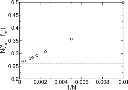
Figure 2: The $O(1/N)$ shift in the free energy is shown (circles). Also shown is the prediction from Eq. (LABEL:84) (dashed line). We use $f(m)=km^{2}/2+1$ and $d(m)=0$ with $k/\mu=2$ and $\mu=5$.

4 The full probability distributions for continuous-time quasispecies theory

In this section we derive the field theoretic expressions for the full probability distribution functions of the parallel and Eigen quasispecies theories. By use of the coherent states formalism, we are able to derive the distribution for arbitrary initial and final conditions. In the long time limit, the initial condition will not matter, as the system will reach a steady state. The final condition matters, though, because the weight assigned by the field theory to a given final condition is exactly equal to the probability that a given surface magnetization occurs in the population of viruses.

4.1 Field theoretic representation of the full probability distribution of the parallel model

To obtain the full probability distribution $P(\{\vec{n}\},t)$, rather than simply the largest Frobenius-Perrone eigenvalue, for the parallel model from Eq. (27) we add a term

$$\delta S=-\sum_{j=1}^{N}[\vec{J}^{*}(j)\cdot\vec{z}_{M}(j)+\vec{J}_{0}(j)\cdot\vec{z}_{0}^{*}(j)]$$ (64)

to the action. We find

$$P(\{\vec{n}\},t)=\sum_{\{\vec{n}_{0}\}}P(\{\vec{n}_{0}\})\left.\prod_{j=1}^{N}\frac{\partial}{\partial J^{*}_{\alpha(j)}(j)}\frac{\partial}{\partial{J_{0}}_{\alpha_{0}(j)}(j)}\right|_{J^{*}=J_{0}=0}{Z}$$ (65)

Here $\alpha(j)=2-n(j)$ is the value of the spin at the final time, and $\alpha_{0}(j)=2-n_{0}(j)$ is the value of the spin at the initial time. Evaluation of this expression is carried out in Appendix E. Here we use the result of Appendix E for a couple different types of initial conditions. We define $Q_{ij}$ to be the matrix element of the matrix $\hat{T}e^{\int_{0}^{t}dt^{\prime}[\mu\sigma_{1}+\bar{\xi}(t^{\prime})\sigma_{3}]}$.

If, for example, we say that at $t=0$, the spins are distributed randomly, but with a given initial surface magnetization, $u_{0}$, then we take the terms in the multinomial expansion of $(Q_{11}+Q_{12}+Q_{21}+Q_{22})^{N}$ that satisfy the initial and final conditions:

$$P(u,t|u_{0}) = \lim_{M\to\infty}\int\left[\prod_{k=1}^{M}\frac{i\epsilon Nd\bar{\xi}_{k}d\xi_{k}}{2\pi}\right]e^{\epsilon\sum_{k=1}^{M}[Nf(\xi_{k})-N\bar{\xi}_{k}\xi_{k}-N\mu+\Delta f]}$$ (66)

$$\times\sum_{j_{1}=\max[0,\frac{N(u_{0}+u)}{2}]}^{\min[N,\frac{N(1+u)}{2},\frac{N(1+u_{0})}{2}]}\frac{N!}{j_{1}!j_{2}!j_{3}!j_{4}!}Q_{11}^{j_{1}}Q_{12}^{j_{2}}Q_{21}^{j_{3}}Q_{22}^{j_{4}}$$

where $j_{1}+j_{2}=N(1+u_{0})/2$, $j_{1}+j_{3}=N(1+u)/2$, and $j_{1}+j_{2}+j_{3}+j_{4}=N$.

Alternatively, if we take an initial condition with spin up and down equally likely ($\langle u_{0}\rangle=0$) and define $Q_{+}=Q_{11}+Q_{21}$ and $Q_{-}=Q_{12}+Q_{22}$ we find

$$P(u,t) = \lim_{M\to\infty}\int\left[\prod_{k=1}^{M}\frac{i\epsilon Nd\bar{\xi}_{k}d\xi_{k}}{2\pi}\right]e^{\epsilon\sum_{k=1}^{M}[Nf(\xi_{k})-N\bar{\xi}_{k}\xi_{k}-N\mu+\Delta f]}$$ (69)

$$\times\left(\begin{array}[]{c}N\\ N(1+u)/2\end{array}\right)Q_{+}[\bar{\xi}]^{N\frac{1+u}{2}}Q_{-}[\bar{\xi}]^{N\frac{1-u}{2}}$$

4.2 The large $N$ limit of the full probability distribution for the parallel model

Since the full probability distribution is also expressed as a functional integral, it can be evaluated by a saddle point in the large $N$ limit. In the saddle point limit, this equation becomes

$$\frac{\ln P(u,t)}{N} = \epsilon\sum_{k=1}^{M}[f(\xi_{k})-\bar{\xi}_{k}\xi_{k}-\mu]-\frac{1+u}{2}\ln\frac{1+u}{2}-\frac{1-u}{2}\ln\frac{1-u}{2}$$ (70)

$$+\frac{1+u}{2}\ln Q_{+}+\frac{1-u}{2}\ln Q_{-}$$

with

$$\bar{\xi}_{k} = f^{\prime}(\xi_{k})$$

$$\xi_{k} = \frac{1+u}{2}\frac{\prod_{l=1}^{k-1}[I+\epsilon\mu\sigma_{1}+\epsilon\bar{\xi}_{l}\sigma_{3}]\sigma_{3}\prod_{l=k+1}^{M}[I+\epsilon\mu\sigma_{1}+\epsilon\bar{\xi}_{l}\sigma_{3}]_{11+21}}{\prod_{l=1}^{M}[I+\epsilon\mu\sigma_{1}+\epsilon\bar{\xi}_{l}\sigma_{3}]_{11+21}}$$ (71)

$$+\frac{1-u}{2}\frac{\prod_{l=1}^{k-1}[I+\epsilon\mu\sigma_{1}+\epsilon\bar{\xi}_{l}\sigma_{3}]\sigma_{3}\prod_{l=k+1}^{M}[I+\epsilon\mu\sigma_{1}+\epsilon\bar{\xi}_{l}\sigma_{3}]_{12+22}}{\prod_{l=1}^{M}[I+\epsilon\mu\sigma_{1}+\epsilon\bar{\xi}_{l}\sigma_{3}]_{12+22}}$$

$$\equiv \frac{1+u}{2}\langle\sigma_{3}(k)\rangle_{+}+\frac{1-u}{2}\langle\sigma_{3}(k)\rangle_{-}$$

In Appendix F we evaluate these expressions where the probability distribution is large, in the Gaussian central region.

4.3 The parallel model distribution function in the Gaussian central region

Adding the terms from Appendix F together, we find that the probability distribution becomes Gaussian in the central region. That is Eq. (70) becomes

$$\frac{\ln P(u,t)}{N} = ({\rm const})-\frac{1}{2}\delta u^{2}\left(\frac{f^{\prime}(u_{*})}{2\mu u_{*}}\right)$$ (72)

We, therefore, conclude that

$$\left\langle\left(u-\langle u\rangle\right)^{2}\right\rangle=\frac{2\mu u_{*}}{Nf^{\prime}(u_{*})}$$ (73)

The fluctuation correction to the fitness is given by

$$\langle f(u)\rangle = f(u_{*})+f^{\prime}(u_{*})\langle u-u_{*}\rangle+\frac{1}{2}f^{\prime\prime}(u_{*})\langle(\delta u)^{2}\rangle+O\left(\frac{1}{N^{2}}\right)$$ (74)

From expressions (47) and (73), we conclude that there is also a shift of the average magnetization for finite $N$:

$$\langle u-u_{*}\rangle = \frac{1}{Nf^{\prime}(u_{*})}\bigg{[}\frac{\mu}{\sqrt{1-\xi_{c}^{2}}}\left[1-\left[1-f^{\prime\prime}(\xi_{c})(1-\xi_{c}^{2})^{3/2}/\mu\right]^{1/2}\right]$$ (75)

$$-\frac{\mu u_{*}f^{\prime\prime}(u_{*})}{f^{\prime}(u_{*})}\bigg{]}$$

4.4 An alternative derivation of the fluctuation corrections to the parallel model distribution function

As an alternative, we may compute averages of the magnetization from the full functional integral expression for the partition function. Computing the surface magnetization From Eq. (69), we find

$$\langle u\rangle(t) = \frac{\sum_{u^{\prime}}u^{\prime}P(u^{\prime},t)}{\sum_{u^{\prime}}P(u^{\prime},t)}$$ (76)

$$= \lim_{M\to\infty}\int\left[\prod_{k=1}^{M}\frac{i\epsilon Nd\bar{\xi}_{k}d\xi_{k}}{2\pi}\right]e^{\epsilon\sum_{k=1}^{M}[Nf(\xi_{k})-N\bar{\xi}_{k}\xi_{k}-N\mu+\Delta f]}$$

$$\times(Q_{+}[\bar{\xi}]+Q_{-}[\bar{\xi}])^{N}\frac{Q_{+}[\bar{\xi}]-Q_{-}[\bar{\xi}]}{Q_{+}[\bar{\xi}]+Q_{-}[\bar{\xi}]}$$

$$\bigg{/}\lim_{M\to\infty}\int\left[\prod_{k=1}^{M}\frac{i\epsilon Nd\bar{\xi}_{k}d\xi_{k}}{2\pi}\right]e^{\epsilon\sum_{k=1}^{M}[Nf(\xi_{k})-N\bar{\xi}_{k}\xi_{k}-N\mu+\Delta f]}$$

$$\times(Q_{+}[\bar{\xi}]+Q_{-}[\bar{\xi}])^{N}$$

This expression, however, is not easily calculated in the saddle point limit.

Computing the fluctuation, we find

$$\langle u^{2}\rangle(t) = \frac{\sum_{u^{\prime}}{u^{\prime}}^{2}P(u^{\prime},t)}{\sum_{u^{\prime}}P(u^{\prime},t)}$$ (77)

$$= \lim_{M\to\infty}\int\left[\prod_{k=1}^{M}\frac{i\epsilon Nd\bar{\xi}_{k}d\xi_{k}}{2\pi}\right]e^{\epsilon\sum_{k=1}^{M}[Nf(\xi_{k})-N\bar{\xi}_{k}\xi_{k}-N\mu+\Delta f]}$$

$$\times(Q_{+}[\bar{\xi}]+Q_{-}[\bar{\xi}])^{N}\left[\frac{(Q_{+}[\bar{\xi}]-Q_{-}[\bar{\xi}])^{2}+4Q_{+}[\bar{\xi}]Q_{-}[\bar{\xi}]/N}{(Q_{+}[\bar{\xi}]+Q_{-}[\bar{\xi}])^{2}}\right]$$

$$\bigg{/}\lim_{M\to\infty}\int\left[\prod_{k=1}^{M}\frac{i\epsilon Nd\bar{\xi}_{k}d\xi_{k}}{2\pi}\right]e^{\epsilon\sum_{k=1}^{M}[Nf(\xi_{k})-N\bar{\xi}_{k}\xi_{k}-N\mu+\Delta f]}$$

$$\times(Q_{+}[\bar{\xi}]+Q_{-}[\bar{\xi}])^{N}$$

This equation implies

$$\left\langle\left(u-\langle u\rangle\right)^{2}\right\rangle=\left\langle\left(\delta\frac{Q_{+}-Q_{-}}{Q_{+}Q_{-}}\right)^{2}\right\rangle+\frac{1-u_{*}^{2}}{N}+O\left(\frac{1}{N^{2}}\right)$$ (78)

The term $(1-u_{*}^{2})/N$ is the variance of the spin at a given site $1\leq i\leq N$. The term $\langle(\delta\Delta Q/Q)^{2}\rangle$, therefore, is $N-1$ times the $O(1/N)$ correlations between spins at any two different sites $1\leq i<j\leq N$. Base compositions at different sites, while equivalent, are not uncorrelated. There is a $O(1/N)$ correlation between base compositions at different sites.

The variance can be written as

$$\left\langle\left(u-\langle u\rangle\right)^{2}\right\rangle=\frac{\int d(\delta u)e^{-Nf^{\prime}(u_{*})\delta u^{2}/(4u_{*})}e^{\delta S}\left(\delta\frac{Q_{+}-Q_{-}}{Q_{+}Q_{-}}\right)^{2}}{\int d(\delta u)e^{-Nf^{\prime}(u_{*})\delta u^{2}/(4u_{*})}e^{\delta S}}$$ (79)

where

$$\delta S/N = \ln(Q_{+}+Q_{-})+\frac{1+u}{2}\ln\frac{1+u}{2}+\frac{1-u}{2}\ln\frac{1-u}{2}$$ (80)

$$-\frac{1+u}{2}\ln Q_{+}-\frac{1-u}{2}\ln Q_{-}$$

We note that

$$\frac{\delta S}{N}=\frac{1}{2}\frac{1-u_{*}^{2}}{4u_{*}^{2}}f^{\prime}(u_{*})^{2}\delta u^{2}+O(\delta u^{3})$$ (81)

Using Eqs. (164), (165), (79), and (81) we find exactly Eq. (73), which shows the consistency of the two calculations. This second calculation, however, makes explicit the contributions of spin-spin correlations to the fluctuation of the population in genome space. Shown in Figure 3 is the comparison between the analytical result of Eq. (73) and a numerical calculation following the algorithm in bb97 .

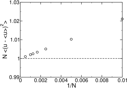
Figure 3: The $O(1/N)$ shift in the variance of the surface magnetization is shown (circles). Also shown is the prediction from Eq. (73) (dashed line). We use $f(m)=km^{2}/2$ with $k/\mu=2$ and $\mu=1$.

4.5 Correlation functions of the parallel model field theory

Since the theory is Gaussian in the saddle point limit, we can evaluate correlations from the inverse of the Hessian in Eq. (45). The inverse is given by

$$\chi = \left(\begin{array}[]{cc}-N\epsilon f^{\prime\prime}(\xi_{c})I&N\epsilon I\\ \epsilon NI&-N\epsilon^{2}\frac{\mu^{2}}{\mu^{2}+\bar{\xi}_{c}^{2}}M+N\epsilon^{2}I\end{array}\right)^{-1}$$ (84)

From Eq. (119) we find

$$\hat{\chi}(k) = \frac{1}{N\epsilon}\left(\begin{array}[]{cc}-f^{\prime\prime}(\xi_{c})&1\\ 1&-\frac{4\epsilon^{2}\mu^{2}}{b}\frac{1}{4b^{2}\epsilon^{2}+k^{2}}+\epsilon\end{array}\right)^{-1}$$ (87)

Inverting this matrix, and inverse Fourier transforming, we find

$$\langle\delta\xi_{k}\delta\xi_{l}\rangle = -\frac{1}{N}\delta_{kl}$$

$$+\frac{1}{N}\frac{1-\xi_{c}^{2}}{\sqrt{1-(1-\xi_{c}^{2})^{3/2}f^{\prime\prime}(\xi_{c})/\mu}}e^{-2\epsilon|k-l|\sqrt{b^{2}-f^{\prime\prime}(\xi_{c})\mu^{2}/b}}$$

$$\langle\delta\bar{\xi}_{k}\delta\bar{\xi}_{l}\rangle = \frac{f^{\prime\prime}(\xi_{c})}{N\epsilon}\delta_{kl}-\frac{f^{\prime\prime}(\xi_{c})^{2}}{N}\delta_{kl}$$

$$+\frac{f^{\prime\prime}(\xi_{c})^{2}}{N}\frac{1-\xi_{c}^{2}}{\sqrt{1-(1-\xi_{c}^{2})^{3/2}f^{\prime\prime}(\xi_{c})/\mu}}e^{-2\epsilon|k-l|\sqrt{b^{2}-f^{\prime\prime}(\xi_{c})\mu^{2}/b}}$$

$$\langle\delta\xi_{k}\delta\bar{\xi}_{l}\rangle = \frac{1}{N\epsilon}\delta_{kl}-\frac{f^{\prime\prime}(\xi_{c})}{N}\delta_{kl}$$

$$+\frac{f^{\prime\prime}(\xi_{c})}{N}\frac{1-\xi_{c}^{2}}{\sqrt{1-(1-\xi_{c}^{2})^{3/2}f^{\prime\prime}(\xi_{c})/\mu}}e^{-2\epsilon|k-l|\sqrt{b^{2}-f^{\prime\prime}(\xi_{c})\mu^{2}/b}}$$

for $k,l\gg 1$ and $k,l\ll M$, where $b=\mu/\sqrt{1-\xi_{c}^{2}}$.

4.6 Field theoretic representation of the full probability distribution of the Eigen model

The full probability distribution for the Eigen model is expressed as a functional integral in an analogous fashion to the parallel model. For the Eigen model we find

$$P(\{\vec{n}\},t) = \lim_{M\to\infty}\int\left[\prod_{k=1}^{M}\frac{i\epsilon Nd\bar{\xi}_{k}d\xi_{k}}{2\pi}\frac{i\epsilon Nd\bar{\eta}_{k}d\eta_{k}}{2\pi}\right]$$ (89)

$$\times e^{\epsilon N\sum_{k=1}^{M}[e^{-\mu+\mu\eta_{k}}f(\xi_{k})-d(\xi_{k})-\bar{\xi}_{k}\xi_{k}-\bar{\eta}_{k}\eta_{k}}$$

$$\times\sum_{\{\vec{n}_{0}\}}P(\{\vec{n}_{0}\})\prod_{j=1}^{N}\{[Q(j)]_{\alpha_{0}(j)\alpha(j)}\}$$

where

$$Q(j) = \prod_{k=1}^{M}[I+\epsilon\bar{\eta}_{k}\sigma_{1}+\epsilon\bar{\xi}_{k}\sigma_{3}]$$ (90)

$$\sim \hat{T}e^{\epsilon\sum_{k=1}^{M}[\bar{\eta}_{k}\sigma_{1}+\bar{\xi}_{k}\sigma_{3}]}$$

$$= \hat{T}e^{\int_{0}^{t}dt^{\prime}[\bar{\eta}(t^{\prime})\sigma_{1}+\bar{\xi}(t^{\prime})\sigma_{3}]}$$

Taking an initial condition with spin up and down equally likely, we find

$$P(u,t) = \lim_{M\to\infty}\int\left[\prod_{k=1}^{M}\frac{i\epsilon Nd\bar{\xi}_{k}d\xi_{k}}{2\pi}\frac{i\epsilon Nd\bar{\eta}_{k}d\eta_{k}}{2\pi}\right]$$ (93)

$$\times e^{\epsilon N\sum_{k=1}^{M}[e^{-\mu+\mu\eta_{k}}f(\xi_{k})-d(\xi_{k})-\bar{\xi}_{k}\xi_{k}-\bar{\eta}_{k}\eta_{k}}$$

$$\times\left(\begin{array}[]{c}N\\ N(1+u)/2\end{array}\right)Q_{+}[\bar{\xi},\bar{\eta}]^{N\frac{1+u}{2}}Q_{-}[\bar{\xi},\bar{\eta}]^{N\frac{1-u}{2}}$$

4.7 The large $N$ limit of the full probability distribution function of the Eigen model

Since the distribution function is expressed as a functional integral, it can be evaluated by the saddle point method. In the saddle point limit, the probability distribution function becomes

$$\frac{\ln P(u,t)}{N} = \epsilon\sum_{k=1}^{M}[e^{-\mu+\mu\eta_{k}}f(\xi_{k})-d(\xi_{k})-\bar{\xi}_{k}\xi_{k}-\bar{\eta}_{k}\eta_{k}]$$ (94)

$$-\frac{1+u}{2}\ln\frac{1+u}{2}-\frac{1-u}{2}\ln\frac{1-u}{2}$$

$$+\frac{1+u}{2}\ln Q_{+}+\frac{1-u}{2}\ln Q_{-}$$

with

$$\bar{\xi}_{k} = e^{-\mu+\mu\eta_{k}}f^{\prime}(\xi_{k})$$

$$\xi_{k} = \frac{1+u}{2}\langle\sigma_{3}(k)\rangle_{+}+\frac{1-u}{2}\langle\sigma_{3}(k)\rangle_{-}$$

$$\bar{\eta}_{k} = \mu e^{-\mu+\mu\eta_{k}}f(\xi_{k})$$

$$\eta_{k} = \frac{1+u}{2}\langle\sigma_{1}(k)\rangle_{+}+\frac{1-u}{2}\langle\sigma_{1}(k)\rangle_{-}$$ (95)

In Appendix G we evaluate these expressions where the probability distribution is large, in the Gaussian central region.

4.8 The Eigen model distribution function in the Gaussian central region

The probability distribution function for the Eigen model becomes Gaussian in the large $N$ limit. Using the results from Appendix G, we find that Eq. (94) becomes

$$\frac{\ln P(u,t)}{N} = ({\rm const})-\frac{1}{2}\delta u^{2}\left(\frac{f^{\prime}(u_{*})-d^{\prime}(u_{*})}{2\mu u_{*}f(u_{*})}\right)$$ (96)

We, therefore, conclude that

$$\left\langle\left(u-\langle u\rangle\right)^{2}\right\rangle=\frac{2\mu u_{*}f(u_{*})}{N[f^{\prime}(u_{*})-d^{\prime}(u_{*})]}$$ (97)

From Eqs. (74), (LABEL:84), and (97) we find the shift of the average magnetization to be

$$\langle u-u_{*}\rangle = \frac{1}{Nf^{\prime}(u_{*})}\bigg{[}b^{\prime}\left[1-\left[1-c^{\prime}/{b^{\prime}}\right]^{1/2}\right]-\frac{\mu u_{*}f(u_{*})f^{\prime\prime}(u_{*})}{f^{\prime}(u_{*})-d^{\prime}(u_{*})}\bigg{]}$$ (98)

Shown in Figure 4 is the comparison between this analytical result and a numerical calculation following the algorithm in ei89 .

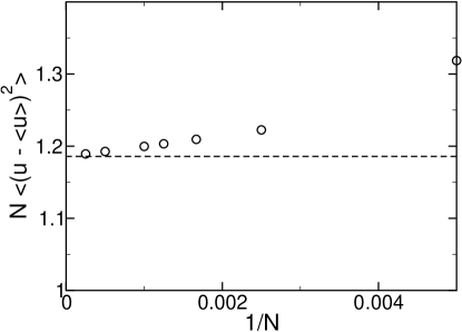
Figure 4: The $O(1/N)$ shift in the variance of the surface magnetization is shown (circles). Also shown is the prediction from Eq. (98) (dashed line). We use $f(m)=km^{2}/2+1$ and $d(m)=0$ with $k/\mu=2$ and $\mu=5$.

5 Conclusion

We have derived exact functional integral representations of the Crow-Kimura and Eigen models of quasispecies theory. The functional integral representation of these quasispecies theories is quite convenient because it allows us to obtain the exact infinite genome solution of these models as well as to obtain the finite length genome corrections. These exact results allow us to discuss the phase transitions that occur in these models as a function of mutation rate. The coherent states derivation of this functional integral also allows us to compute the full time-dependent probability distribution function of the population in sequence space, including the dependence on initial and final conditions.

The functional integral representation leads to an interacting field theory for spin and mutation fields. In the limit of long genomes, the field theory becomes Gaussian. We have evaluated the theory in the infinite genome limit to give the mean replication rate for arbitrary replication and degradation functions. These results were used to exhibit the phase transitions that occur in quasispecies theory as a function of mutation rate. For smooth replication and degradation rate functions, we have evaluated the $O(1/N)$ corrections to the mean replication rate. We have also derived the finite, $O(1/\sqrt{N})$ width of the virus population in genome space in this limit.

The functional integral representation can be applied to generalizations of the quasispecies theories considered here. The extension of the present results to arbitrary replication and degradation functions that depend on distances from $K$ points in the space of all possible genomes is straightforward with the introduction of overlap parameters Deem2006 . With the Schwinger spin coherent state formalism, the extension to genomes with alphabets larger than binary Burger is also straightforward, since the field theory in ${\bf z}^{*}$ and ${\bf z}$ remains Gaussian due to constraint (4).

Appendix A

To evaluate the partition function of the parallel model, we introduce $\xi_{k}=\frac{1}{N}\sum_{j=1}^{N}{\vec{z}}^{*}_{k}(j)\sigma_{3}{\vec{z}}_{k-1}(j)$ with the representation

$$\int{\cal D}\xi\prod_{k=1}^{M}\delta\left[\xi_{k}-\frac{1}{N}\sum_{j=1}^{N}{\vec{z}}^{*}_{k}(j)\sigma_{3}{\vec{z}}_{k-1}(j)\right]$$

$$=\int\left[\prod_{k=1}^{M}\frac{d\bar{\xi}_{k}d\xi_{k}}{2\pi}\right]e^{i\sum_{k=1}^{M}\bar{\xi}_{k}\xi_{k}-\frac{i}{N}\sum_{k=1}^{M}\vec{z}^{*}_{k}(j)\bar{\xi}_{k}\sigma_{3}\vec{z}_{k-1}(j)}$$

$$=\int\left[\prod_{k=1}^{M}\frac{i\epsilon Nd\bar{\xi}_{k}d\xi_{k}}{2\pi}\right]e^{-\epsilon N\sum_{k=1}^{M}\bar{\xi}_{k}\xi_{k}+\epsilon\sum_{k=1}^{M}\vec{z}^{*}_{k}(j)\bar{\xi}_{k}\sigma_{3}\vec{z}_{k-1}(j)}$$ (99)

We thus find

$${Z} = \lim_{M\to\infty}\int\left[\prod_{k=1}^{M}\frac{i\epsilon Nd\bar{\xi}_{k}d\xi_{k}}{2\pi}\right]e^{\epsilon\sum_{k=1}^{M}[Nf(\xi_{k})-N\bar{\xi}_{k}\xi_{k}-N\mu+\Delta f]}$$ (100)

$$\times\int{\cal D}\lambda{\cal D}\vec{z}^{*}{\cal D}\vec{z}\prod_{j=1}^{N}e^{-i\lambda_{j}}e^{-\sum_{k,l=1}^{M}\vec{z}_{k}^{*}(j)S(j)_{kl}\vec{z}_{l}(j)}|_{\{\vec{z}_{0}\}=\{e^{i\lambda}\vec{z}_{M}\}}$$

$$= \lim_{M\to\infty}\int\left[\prod_{k=1}^{M}\frac{i\epsilon Nd\bar{\xi}_{k}d\xi_{k}}{2\pi}\right]e^{\epsilon\sum_{k=1}^{M}[Nf(\xi_{k})-N\bar{\xi}_{k}\xi_{k}-N\mu+\Delta f]}$$

$$\times\int{\cal D}\lambda\prod_{j=1}^{N}e^{-i\lambda_{j}}[\det S(j)]^{-1}$$

The matrix $S(j)$ has the form

$$S(j)=\left(\begin{array}[]{ccccc}I&0&0&\ldots&-e^{i\lambda_{j}}A_{1}(j)\\ -A_{2}(j)&I&0&\ldots&0\\ 0&-A_{3}(j)&I&\ldots&0\\ &&&\ddots\\ 0&&\ldots&-A_{M}(j)&I\end{array}\right)$$ (106)

where $A_{k}(j)=I+\epsilon\mu\sigma_{1}+\epsilon\bar{\xi}_{k}\sigma_{3}$. We find

$$\det S(j) = \det\left[I-e^{i\lambda_{j}}\prod_{k=1}^{M}A_{k}(j)\right]$$ (107)

$$= \det\left[I-e^{i\lambda_{j}}\hat{T}e^{\epsilon\sum_{k=1}^{M}[\mu\sigma_{1}+\bar{\xi}_{k}\sigma_{3}]}\right]$$

$$= e^{{\rm Tr}\ln\left[I-{e^{i\lambda_{j}}}\hat{T}e^{\epsilon\sum_{k=1}^{M}[\mu\sigma_{1}+\bar{\xi}_{k}\sigma_{3}]}\right]}$$

Here the operator $\hat{T}$ indicates time ordering. The partition function becomes

$${Z} = \lim_{M\to\infty}\int\left[\prod_{k=1}^{M}\frac{i\epsilon Nd\bar{\xi}_{k}d\xi_{k}}{2\pi}\right]e^{\epsilon\sum_{k=1}^{M}[Nf(\xi_{k})-N\bar{\xi}_{k}\xi_{k}-N\mu+\Delta f]}$$ (108)

$$\times\int{\cal D}\lambda\prod_{j=1}^{N}e^{-i\lambda_{j}}e^{-{\rm Tr}\ln\left[I-{e^{i\lambda_{j}}}\hat{T}e^{\epsilon\sum_{k=1}^{M}[\mu\sigma_{1}+\bar{\xi}_{k}\sigma_{3}]}\right]}$$

$$= \lim_{M\to\infty}\int\left[\prod_{k=1}^{M}\frac{i\epsilon Nd\bar{\xi}_{k}d\xi_{k}}{2\pi}\right]e^{\epsilon\sum_{k=1}^{M}[Nf(\xi_{k})-N\bar{\xi}_{k}\xi_{k}-N\mu+\Delta f]}$$

$$\times\prod_{j=1}^{N}Q(j)$$

where

$$Q(j) = {\rm Tr}\prod_{k=1}^{M}[I+\epsilon\mu\sigma_{1}+\epsilon\bar{\xi}_{k}\sigma_{3}]$$ (109)

$$\sim {\rm Tr}\hat{T}e^{\epsilon\sum_{k=1}^{M}[\mu\sigma_{1}+\bar{\xi}_{k}\sigma_{3}]}$$

$$= {\rm Tr}\hat{T}e^{\int_{0}^{t}dt^{\prime}[\mu\sigma_{1}+\bar{\xi}(t^{\prime})\sigma_{3}]}$$

Appendix B

In this Appendix we evaluate the fluctuation corrections to the parallel model. The second term in the last derivative of Eq. (45) is given by

$$\frac{{\rm Tr}\sigma_{3}e^{\epsilon M(\mu\sigma_{1}+\bar{\xi}_{c}\sigma_{3})}}{{\rm Tr}e^{\epsilon M(\mu\sigma_{1}+\bar{\xi}_{c}\sigma_{3})}} = \frac{\bar{\xi}_{c}}{[\mu^{2}+\bar{\xi}_{c}^{2}]^{1/2}}\tanh t[\mu^{2}+\bar{\xi}_{c}^{2}]^{1/2}$$ (110)

$$\sim \frac{\bar{\xi}_{c}}{[\mu^{2}+\bar{\xi}_{c}^{2}]^{1/2}}{\rm~{}as~{}}t\to\infty$$

The first term in the last derivative is given for $k\neq l$ by

$$\frac{{\rm Tr}\sigma_{3}e^{\epsilon|l-k|(\mu\sigma_{1}+\bar{\xi}_{c}\sigma_{3})}\sigma_{3}e^{\epsilon(M-|l-k|)(\mu\sigma_{1}+\bar{\xi}_{c}\sigma_{3})}}{{\rm Tr}e^{\epsilon M(\mu\sigma_{1}+\bar{\xi}_{c}\sigma_{3})}}$$

$$=\frac{\bar{\xi}_{c}^{2}}{\mu^{2}+\bar{\xi}_{c}^{2}}+\frac{\mu^{2}}{\mu^{2}+\bar{\xi}_{c}^{2}}\frac{\cosh(t_{1}-t_{2})\sqrt{\mu^{2}+\bar{\xi}_{c}^{2}}}{\cosh t\sqrt{\mu^{2}+\bar{\xi}_{c}^{2}}}$$

$$\sim\frac{\bar{\xi}_{c}^{2}}{\mu^{2}+\bar{\xi}_{c}^{2}}+\frac{\mu^{2}}{\mu^{2}+\bar{\xi}_{c}^{2}}e^{(|t_{1}-t_{2}|-t)\sqrt{\mu^{2}+\bar{\xi}_{c}^{2}}}{\rm~{}as~{}}t\to\infty$$ (111)

where $t_{1}=\epsilon|l-k|$ and $t_{2}=\epsilon(M-|l-k|)$. For $k=l$, the first term in the last derivative is zero from the first line of Eq. (109). We find

$$\frac{\partial^{2}S}{\partial\bar{\xi}_{k}\partial\bar{\xi}_{l}}=-N\epsilon^{2}\frac{\mu^{2}}{\mu^{2}+\bar{\xi}_{c}^{2}}M_{kl}+N\epsilon^{2}\delta_{kl}$$ (112)

where

$$M_{kl}=e^{\epsilon[|M-2|l-k||-M]\sqrt{\mu^{2}+\bar{\xi}_{c}^{2}}}$$ (113)

We let $\bar{\eta}_{k}=\delta\bar{\xi}_{k}\sqrt{(}\epsilon N)$ and $\eta_{k}=\delta\xi_{k}\sqrt{(}\epsilon N)$, and the partition function becomes

$${Z} = e^{-S(\bar{\xi}_{c},\xi_{c})}\lim_{M\to\infty}\int\left[\prod_{k=1}^{M}\frac{id\bar{\eta}_{k}d\eta_{k}}{2\pi}\right]e^{\frac{1}{2}\sum_{k}[f^{\prime\prime}(\xi_{c})\eta_{k}^{2}-2\bar{\eta}_{k}\eta_{k}]}$$ (114)

$$\times e^{\frac{1}{2}\sum_{k,l}\left[\epsilon\frac{\mu^{2}}{\mu^{2}+\bar{\xi}_{c}^{2}}M_{kl}\bar{\eta}_{k}\bar{\eta}_{l}-\epsilon\bar{\eta}_{k}\bar{\eta}_{l}\delta_{kl}\right]}$$

We let $\eta_{k}^{\prime}=i\eta_{k}\sqrt{f^{\prime\prime}(\xi_{c})}$ and $\bar{\eta}_{k}^{\prime}=\bar{\eta}_{k}/\sqrt{f^{\prime\prime}(\xi_{c})}$ to obtain

$${Z} = e^{-S(\bar{\xi}_{c},\xi_{c})}\lim_{M\to\infty}\int\left[\prod_{k=1}^{M}\frac{d\bar{\eta}_{l}^{\prime}d\eta_{l}^{\prime}}{2\pi}\right]e^{-\frac{1}{2}\sum_{k}{\eta_{l}^{\prime}}^{2}+i\sum_{k}\bar{\eta}_{l}^{\prime}\eta_{l}^{\prime}}$$ (115)

$$\times e^{\frac{1}{2}\sum_{k,l}\left[\epsilon\frac{\mu^{2}f^{\prime\prime}(\xi_{c})}{\mu^{2}+\bar{\xi}_{c}^{2}}M_{kl}\bar{\eta}_{k}^{\prime}\bar{\eta}_{l}^{\prime}-\epsilon f^{\prime\prime}(\xi_{c})\bar{\eta}_{k}^{\prime}\bar{\eta}_{l}^{\prime}\delta_{kl}\right]}$$

Integrating over $\eta^{\prime}$, we find

$${Z} = e^{-S(\bar{\xi}_{c},\xi_{c})}\lim_{M\to\infty}\int\left[\prod_{k=1}^{M}\frac{d\bar{\eta}_{l}^{\prime}}{\sqrt{2\pi}}\right]e^{-\frac{1}{2}\sum_{k,l}\left[\delta_{kl}-\epsilon\frac{\mu^{2}f^{\prime\prime}(\xi_{c})}{\mu^{2}+\bar{\xi}_{c}^{2}}M_{kl}+\epsilon f^{\prime\prime}(\xi_{c})\delta_{kl}\right]\bar{\eta}_{k}^{\prime}\bar{\eta}_{l}^{\prime}}$$ (116)

$$= e^{-S(\bar{\xi}_{c},\xi_{c})}\lim_{M\to\infty}\int\left[\prod_{k=1}^{M}\frac{d\bar{\eta}_{l}^{\prime}}{\sqrt{2\pi}}\right]e^{-\frac{1}{2}\sum_{k,l}\bar{\eta}_{l}^{\prime}F_{kl}\bar{\eta}_{l}^{\prime}}$$

$$= e^{-S(\bar{\xi}_{c},\xi_{c})}(\det F)^{-1/2}$$

where

$$F_{kl} = \delta_{kl}-\epsilon\frac{\mu^{2}f^{\prime\prime}(\xi_{c})}{\mu^{2}+\bar{\xi}_{c}^{2}}M_{kl}+\epsilon f^{\prime\prime}(\xi_{c})\delta_{kl}$$ (117)

$$= \delta_{kl}-\epsilon\frac{a}{b^{2}}M_{kl}+\epsilon f^{\prime\prime}(\xi_{c})\delta_{kl}$$

where $a=\mu^{2}f^{\prime\prime}(\xi_{c})$ and $b^{2}=\mu^{2}+\bar{\xi}_{c}^{2}$. We define $F^{\prime}$, where $F_{kl}=F_{kl}^{\prime}+\epsilon f^{\prime\prime}(\xi_{c})\delta_{kl}$. We note that

$$\det F = \det[I+\epsilon f^{\prime\prime}(\xi_{c})I-\epsilon\frac{a}{b^{2}}M]$$ (118)

$$= (\det[I+\epsilon f^{\prime\prime}(\xi_{c})I])(\det[I-\epsilon\frac{a}{b^{2}}M[I+\epsilon f^{\prime\prime}(\xi_{c})I]^{-1})$$

$$\sim (\det[I+\epsilon f^{\prime\prime}(\xi_{c})I])(\det[I-\epsilon\frac{a}{b^{2}}M])$$

$$= (\det F^{\prime})e^{{\rm Tr}~{}\ln[I+\epsilon f^{\prime\prime}(\xi_{c})]}$$

$$\sim (\det F^{\prime})e^{{\rm Tr}~{}\epsilon f^{\prime\prime}(\xi_{c})I}$$

$$= (\det F^{\prime})e^{tf^{\prime\prime}(\xi_{c})}$$

To evaluate $\det F^{\prime}$ we use Fourier space. We find

$$\hat{F}^{\prime}(k)=1-\frac{4\epsilon^{2}a}{b}\frac{1}{4b^{2}\epsilon^{2}+k^{2}}$$ (119)

and

$$\det F^{\prime} = \prod_{i}\lambda_{i}=\prod_{k}\hat{F}^{\prime}(k)$$ (120)

where $k=2\pi n/M=2\pi\epsilon n/t$, $n=-M/2,\ldots,(M-1)/2$. In the limit of infinite $M$, we find

$$\det F^{\prime} = \frac{\left(\sinh t\sqrt{b^{2}-a/b}\right)^{2}}{\left(\sinh bt\right)^{2}}$$ (121)

$$= \frac{\left(\sinh t\left[\mu^{2}+\bar{\xi}_{c}^{2}-\mu^{2}f^{\prime\prime}(\xi_{c})/\sqrt{\mu^{2}+\bar{\xi}_{c}^{2}}\right]^{1/2}\right)^{2}}{\left(\sinh t\sqrt{\mu^{2}+\bar{\xi}_{c}^{2}}\right)^{2}}$$

$$\sim e^{-2t\left[\sqrt{\mu^{2}+\bar{\xi}_{c}^{2}}-[\mu^{2}+\bar{\xi}_{c}^{2}-\mu^{2}f^{\prime\prime}(\xi_{c})/\sqrt{\mu^{2}+\bar{\xi}_{c}^{2}}]^{1/2}\right]^{1/2}}{\rm~{}as~{}}t\to\infty$$

Using Eq. (43), (116), (121), and (118) we find the mean replication rate at large time becomes

$$\frac{\ln Z}{tN} = f(\xi_{c})-\bar{\xi}_{c}\xi_{c}+\sqrt{\mu^{2}+\bar{\xi}_{c}^{2}}-\mu+\frac{\Delta f}{N}-\frac{f^{\prime\prime}(\xi_{c})}{2N}$$ (122)

$$+\frac{1}{N}\frac{\mu}{\sqrt{1-\xi_{c}^{2}}}\left[1-\left[1-f^{\prime\prime}(\xi_{c})(1-\xi_{c}^{2})^{3/2}/\mu\right]^{1/2}\right]$$

with

$$\bar{\xi}_{c} = f^{\prime}(\xi_{c})$$

$$\xi_{c} = \frac{\bar{\xi}_{c}}{[\mu^{2}+\bar{\xi}_{c}^{2}]^{1/2}}\tanh t[\mu^{2}+\bar{\xi}_{c}^{2}]^{1/2}$$ (123)

Appendix C

To evaluate the partition function of the Eigen model, we define magnetization and mutation fields with $\xi_{k}=\frac{1}{N}\sum_{j=1}^{N}{\vec{z}}^{*}_{k}(j)\sigma_{3}{\vec{z}}_{k-1}(j)$ and $\eta_{k}=\frac{1}{N}\sum_{j=1}^{N}{\vec{z}}^{*}_{k}(j)\sigma_{1}{\vec{z}}_{k-1}(j)$ to write the partition function for the Eigen model as

$${Z} = \lim_{M\to\infty}\int\left[\prod_{k=1}^{M}\frac{i\epsilon Nd\bar{\xi}_{k}d\xi_{k}}{2\pi}\right]\left[\prod_{k=1}^{M}\frac{i\epsilon Nd\bar{\eta}_{k}d\eta_{k}}{2\pi}\right]$$ (124)

$$\times e^{\epsilon N\sum_{k=1}^{M}[e^{-\mu_{1}}e^{\mu\eta_{k}}f(\xi_{k})-d(\xi_{k})-\bar{\xi}_{k}\xi_{k}-\bar{\eta}_{k}\eta_{k}]}$$

$$\times\int{\cal D}\lambda{\cal D}\vec{z}^{*}{\cal D}\vec{z}\prod_{j=1}^{N}e^{-i\lambda_{j}}e^{-\sum_{k,l=1}^{M}\vec{z}_{k}^{*}(j)S(j)_{kl}\vec{z}_{l}(j)}|_{\{\vec{z}_{0}\}=\{e^{i\lambda}\vec{z}_{M}\}}$$

$$= \lim_{M\to\infty}\int\left[\prod_{k=1}^{M}\frac{i\epsilon Nd\bar{\xi}_{k}d\xi_{k}}{2\pi}\right]\left[\prod_{k=1}^{M}\frac{i\epsilon Nd\bar{\eta}_{k}d\eta_{k}}{2\pi}\right]$$

$$e^{\epsilon N\sum_{k=1}^{M}[e^{-\mu_{1}}e^{\mu\eta_{k}}f(\xi_{k})-d(\xi_{k})-\bar{\xi}_{k}\xi_{k}-\bar{\eta}_{k}\eta_{k}]}$$

$$\times\int[{\cal D}\lambda]e^{-i\lambda_{j}}\prod_{j=1}^{N}[\det S(j)]^{-1}$$

The matrix $S(j)$ has the form of Eq. (106) with $A_{k}(j)=I+\epsilon\bar{\eta}_{k}\sigma_{1}+\epsilon\bar{\xi}_{k}\sigma_{3}$. The determinant and constraint evaluate as in Eqs. (107–108) to give

$${Z}=\lim_{M\to\infty}\int \left[\prod_{k=1}^{M}\frac{i\epsilon Nd\bar{\xi}_{k}d\xi_{k}}{2\pi}\right]\left[\prod_{k=1}^{M}\frac{i\epsilon Nd\bar{\eta}_{k}d\eta_{k}}{2\pi}\right]$$ (125)

$$\times e^{\epsilon N\sum_{k=1}^{M}[e^{-\mu_{1}}e^{\mu\eta_{k}}f(\xi_{k})-d(\xi_{k})-\bar{\xi}_{k}\xi_{k}-\bar{\eta}_{k}\eta_{k}]}$$

$$\times\prod_{j=1}^{N}Q(j)$$

where

$$Q(j) = {\rm Tr}\prod_{k=1}^{N}[I+\epsilon\bar{\eta}_{k}\sigma_{1}+\epsilon\bar{\xi}_{k}\sigma_{3}]$$ (126)

$$\sim {\rm Tr}\hat{T}e^{\epsilon\sum_{k=1}^{M}[\bar{\eta}_{k}\sigma_{1}+\bar{\xi}_{k}\sigma_{3}]}$$

$$= {\rm Tr}\hat{T}e^{\int_{0}^{t}dt^{\prime}[\bar{\eta}(t^{\prime})\sigma_{1}+\bar{\xi}(t^{\prime})\sigma_{3}]}$$

Appendix D

We here determine the fluctuation corrections to the mean excess replication rate per site, $(\ln Z)/(tN)$, in the Eigen model. We expand the action around the saddle point limit

$$S[\bar{\xi},\xi,\bar{\eta},\eta] = S(\bar{\xi}_{c},\xi_{c},\bar{\eta}_{c},\eta_{c})+\frac{1}{2}\sum_{k,l=1}^{M}\bigg{[}\left.\frac{\partial^{2}S}{\partial\xi_{k}\partial\xi_{l}}\right|_{\bar{\xi}_{c},\xi_{c},\bar{\eta}_{c},\eta_{c}}\delta\xi_{k}\delta\xi_{l}$$

$$+2\left.\frac{\partial^{2}S}{\partial\xi_{k}\partial\bar{\xi}_{l}}\right|_{\bar{\xi}_{c},\xi_{c},\bar{\eta}_{c},\eta_{c}}\delta\xi_{k}\delta\bar{\xi}_{l}+\left.\frac{\partial^{2}S}{\partial\bar{\xi}_{k}\partial\bar{\xi}_{l}}\right|_{\bar{\xi}_{c},\xi_{c},\bar{\eta}_{c},\eta_{c}}\delta\bar{\xi}_{k}\delta\bar{\xi}_{l}$$

$$+\left.\frac{\partial^{2}S}{\partial\eta_{k}\partial\eta_{l}}\right|_{\bar{\xi}_{c},\xi_{c},\bar{\eta}_{c},\eta_{c}}\delta\eta_{k}\delta\eta_{l}+2\left.\frac{\partial^{2}S}{\partial\eta_{k}\partial\bar{\eta}_{l}}\right|_{\bar{\xi}_{c},\xi_{c},\bar{\eta}_{c},\eta_{c}}\delta\eta_{k}\delta\bar{\eta}_{l}$$

$$+\left.\frac{\partial^{2}S}{\partial\bar{\eta}_{k}\partial\bar{\eta}_{l}}\right|_{\bar{\xi}_{c},\xi_{c},\bar{\eta}_{c},\eta_{c}}\delta\bar{\eta}_{k}\delta\bar{\eta}_{l}$$

$$+2\left.\frac{\partial^{2}S}{\partial\xi_{k}\partial\bar{\eta}_{l}}\right|_{\bar{\xi}_{c},\xi_{c},\bar{\eta}_{c},\eta_{c}}\delta\xi_{k}\delta\bar{\eta}_{l}+2\left.\frac{\partial^{2}S}{\partial\eta_{k}\partial\bar{\xi}_{l}}\right|_{\bar{\xi}_{c},\xi_{c},\bar{\eta}_{c},\eta_{c}}\delta\eta_{k}\delta\bar{\xi}_{l}$$

$$+2\left.\frac{\partial^{2}S}{\partial\xi_{k}\partial\eta_{l}}\right|_{\bar{\xi}_{c},\xi_{c},\bar{\eta}_{c},\eta_{c}}\delta\xi_{k}\delta\eta_{l}+2\left.\frac{\partial^{2}S}{\partial\bar{\eta}_{k}\partial\bar{\xi}_{l}}\right|_{\bar{\xi}_{c},\xi_{c},\bar{\eta}_{c},\eta_{c}}\delta\bar{\eta}_{k}\delta\bar{\xi}_{l}\bigg{]}$$

We find

$$\left.\frac{\partial^{2}S}{\partial\xi_{k}\partial\xi_{l}}\right|_{\bar{\xi}_{c},\xi_{c},\bar{\eta}_{c},\eta_{c}} = -N\epsilon e^{-mu_{1}+\mu\eta_{c}}f^{\prime\prime}(\xi_{c})\delta_{kl}+N\epsilon d^{\prime\prime}(\xi_{c})\delta_{kl}$$

$$\left.\frac{\partial^{2}S}{\partial\xi_{k}\partial\eta_{l}}\right|_{\bar{\xi}_{c},\xi_{c},\bar{\eta}_{c},\eta_{c}} = -N\epsilon\mu e^{-mu_{1}+\mu\eta_{c}}f^{\prime}(\xi_{c})\delta_{kl}$$

$$\left.\frac{\partial^{2}S}{\partial\eta_{k}\partial\eta_{l}}\right|_{\bar{\xi}_{c},\xi_{c},\bar{\eta}_{c},\eta_{c}} = -N\epsilon\mu^{2}e^{-mu_{1}+\mu\eta_{c}}f(\xi_{c})\delta_{kl}$$

$$\left.\frac{\partial^{2}S}{\partial\xi_{k}\partial\bar{\xi}_{l}}\right|_{\bar{\xi}_{c},\xi_{c},\bar{\eta}_{c},\eta_{c}} = \epsilon N\delta_{kl}$$

$$\left.\frac{\partial^{2}S}{\partial\eta_{k}\partial\bar{\eta}_{l}}\right|_{\bar{\xi}_{c},\xi_{c},\bar{\eta}_{c},\eta_{c}} = \epsilon N\delta_{kl}$$

$$\left.\frac{\partial^{2}S}{\partial\bar{\xi}_{k}\partial\bar{\xi}_{l}}\right|_{\bar{\xi}_{c},\xi_{c},\bar{\eta}_{c},\eta_{c}} = -N\epsilon^{2}\frac{{\rm Tr}\sigma_{3}e^{\epsilon|l-k|(\bar{\eta}_{c}\sigma_{1}+\bar{\xi}_{c}\sigma_{3})}\sigma_{3}e^{\epsilon(M-|l-k|(\bar{\eta}_{c}\sigma_{1}+\bar{\xi}_{c}\sigma_{3})}}{{\rm Tr}e^{\epsilon M(\bar{\eta}_{c}\sigma_{1}+\bar{\xi}_{c}\sigma_{3})}}(1-\delta_{kl})$$

$$+N\epsilon^{2}\left(\frac{{\rm Tr}\sigma_{3}e^{\epsilon M(\bar{\eta}_{c}\sigma_{1}+\bar{\xi}_{c}\sigma_{3})}}{{\rm Tr}e^{\epsilon M(\bar{\eta}_{c}\sigma_{1}+\bar{\xi}_{c}\sigma_{3})}}\right)^{2}$$

$$\left.\frac{\partial^{2}S}{\partial\bar{\eta}_{k}\partial\bar{\eta}_{l}}\right|_{\bar{\xi}_{c},\xi_{c},\bar{\eta}_{c},\eta_{c}} = -N\epsilon^{2}\frac{{\rm Tr}\sigma_{1}e^{\epsilon|l-k|(\bar{\eta}_{c}\sigma_{1}+\bar{\eta}_{c}\sigma_{3})}\sigma_{1}e^{\epsilon(M-|l-k|(\bar{\eta}_{c}\sigma_{1}+\bar{\eta}_{c}\sigma_{3})}}{{\rm Tr}e^{\epsilon M(\bar{\eta}_{c}\sigma_{1}+\bar{\eta}_{c}\sigma_{3})}}(1-\delta_{kl})$$

$$+N\epsilon^{2}\left(\frac{{\rm Tr}\sigma_{1}e^{\epsilon M(\bar{\eta}_{c}\sigma_{1}+\bar{\eta}_{c}\sigma_{3})}}{{\rm Tr}e^{\epsilon M(\bar{\eta}_{c}\sigma_{1}+\bar{\eta}_{c}\sigma_{3})}}\right)^{2}$$

$$\left.\frac{\partial^{2}S}{\partial\bar{\eta}_{k}\partial\bar{\xi}_{l}}\right|_{\bar{\xi}_{c},\xi_{c},\bar{\eta}_{c},\eta_{c},l\geq k} = -N\epsilon^{2}\frac{{\rm Tr}\sigma_{3}e^{\epsilon(l-k)(\bar{\eta}_{c}\sigma_{1}+\bar{\xi}_{c}\sigma_{3})}\sigma_{1}e^{\epsilon(M-l+k)(\bar{\eta}_{c}\sigma_{1}+\bar{\xi}_{c}\sigma_{3})}}{{\rm Tr}e^{\epsilon M(\bar{\eta}_{c}\sigma_{1}+\bar{\xi}_{c}\sigma_{3})}}(1-\delta_{kl})$$

$$+N\epsilon^{2}\left(\frac{{\rm Tr}\sigma_{1}e^{\epsilon M(\bar{\eta}_{c}\sigma_{1}+\bar{\xi}_{c}\sigma_{3})}}{{\rm Tr}e^{\epsilon M(\bar{\eta}_{c}\sigma_{1}+\bar{\xi}_{c}\sigma_{3})}}\right)\left(\frac{{\rm Tr}\sigma_{3}e^{\epsilon M(\bar{\eta}_{c}\sigma_{1}+\bar{\xi}_{c}\sigma_{3})}}{{\rm Tr}e^{\epsilon M(\bar{\eta}_{c}\sigma_{1}+\bar{\xi}_{c}\sigma_{3})}}\right)$$

$$\left.\frac{\partial^{2}S}{\partial\bar{\eta}_{k}\partial\bar{\xi}_{l}}\right|_{\bar{\xi}_{c},\xi_{c},\bar{\eta}_{c},\eta_{c},l\leq k} = -N\epsilon^{2}\frac{{\rm Tr}\sigma_{1}e^{\epsilon(k-l)(\bar{\eta}_{c}\sigma_{1}+\bar{\xi}_{c}\sigma_{3})}\sigma_{3}e^{\epsilon(M-k+l)(\bar{\eta}_{c}\sigma_{1}+\bar{\xi}_{c}\sigma_{3})}}{{\rm Tr}e^{\epsilon M(\bar{\eta}_{c}\sigma_{1}+\bar{\xi}_{c}\sigma_{3})}}(1-\delta_{kl})$$

$$+N\epsilon^{2}\left(\frac{{\rm Tr}\sigma_{1}e^{\epsilon M(\bar{\eta}_{c}\sigma_{1}+\bar{\xi}_{c}\sigma_{3})}}{{\rm Tr}e^{\epsilon M(\bar{\eta}_{c}\sigma_{1}+\bar{\xi}_{c}\sigma_{3})}}\right)\left(\frac{{\rm Tr}\sigma_{3}e^{\epsilon M(\bar{\eta}_{c}\sigma_{1}+\bar{\xi}_{c}\sigma_{3})}}{{\rm Tr}e^{\epsilon M(\bar{\eta}_{c}\sigma_{1}+\bar{\xi}_{c}\sigma_{3})}}\right)$$

The other two derivatives in Eq. (LABEL:70) are zero. We find

$$\frac{{\rm Tr}\sigma_{3}e^{\epsilon M(\bar{\eta}_{c}\sigma_{1}+\bar{\xi}_{c}\sigma_{3})}}{{\rm Tr}e^{\epsilon M(\bar{\eta}_{c}\sigma_{1}+\bar{\xi}_{c}\sigma_{3})}} = \frac{\bar{\xi}_{c}}{[\bar{\eta}_{c}^{2}+\bar{\xi}_{c}^{2}]^{1/2}}\tanh t[\bar{\eta}_{c}^{2}+\bar{\xi}_{c}^{2}]^{1/2}$$ (129)

$$\sim \frac{\bar{\xi}_{c}}{[\bar{\eta}_{c}^{2}+\bar{\xi}_{c}^{2}]^{1/2}}{\rm~{}as~{}}t\to\infty$$

and

$$\frac{{\rm Tr}\sigma_{3}e^{\epsilon|l-k|(\bar{\eta}_{c}\sigma_{1}+\bar{\xi}_{c}\sigma_{3})}\sigma_{3}e^{\epsilon(M-|l-k|)(\bar{\eta}_{c}\sigma_{1}+\bar{\xi}_{c}\sigma_{3})}}{{\rm Tr}e^{\epsilon M(\bar{\eta}_{c}\sigma_{1}+\bar{\xi}_{c}\sigma_{3})}}$$

$$=\frac{\bar{\xi}_{c}^{2}}{\bar{\eta}_{c}^{2}+\bar{\xi}_{c}^{2}}+\frac{\bar{\eta}_{c}^{2}}{\bar{\eta}_{c}^{2}+\bar{\xi}_{c}^{2}}\frac{\cosh(t_{1}-t_{2})\sqrt{\bar{\eta}_{c}^{2}+\bar{\xi}_{c}^{2}}}{\cosh t\sqrt{\bar{\eta}_{c}^{2}+\bar{\xi}_{c}^{2}}}$$

$$\sim\frac{\bar{\xi}_{c}^{2}}{\bar{\eta}_{c}^{2}+\bar{\xi}_{c}^{2}}+\frac{\bar{\eta}_{c}^{2}}{\bar{\eta}_{c}^{2}+\bar{\xi}_{c}^{2}}e^{(|t_{1}-t_{2}|-t)\sqrt{\bar{\eta}_{c}^{2}+\bar{\xi}_{c}^{2}}}{\rm~{}as~{}}t\to\infty$$ (130)

where $t_{1}=\epsilon|l-k|$ and $t_{2}=\epsilon(M-|l-k|)$. We find

$$\frac{\partial^{2}S}{\partial\bar{\xi}_{k}\partial\bar{\xi}_{l}}=-N\epsilon^{2}\frac{\bar{\eta}_{c}^{2}}{\bar{\eta}_{c}^{2}+\bar{\xi}_{c}^{2}}M^{\prime}_{kl}+N\epsilon^{2}\delta_{kl}$$ (131)

where

$$M^{\prime}_{kl}=e^{\epsilon[|M-2|l-k||-M]\sqrt{\bar{\eta}_{c}^{2}+\bar{\xi}_{c}^{2}}}$$ (132)

The other traces evaluate as

$$\frac{{\rm Tr}\sigma_{1}e^{\epsilon M(\bar{\eta}_{c}\sigma_{1}+\bar{\xi}_{c}\sigma_{3})}}{{\rm Tr}e^{\epsilon M(\bar{\eta}_{c}\sigma_{1}+\bar{\xi}_{c}\sigma_{3})}} = \frac{\bar{\eta}_{c}}{[\bar{\eta}_{c}^{2}+\bar{\xi}_{c}^{2}]^{1/2}}\tanh t[\bar{\eta}_{c}^{2}+\bar{\xi}_{c}^{2}]^{1/2}$$ (133)

$$\sim \frac{\bar{\eta}_{c}}{[\bar{\eta}_{c}^{2}+\bar{\xi}_{c}^{2}]^{1/2}}{\rm~{}as~{}}t\to\infty$$

and

$$\frac{{\rm Tr}\sigma_{1}e^{\epsilon|l-k|(\bar{\eta}_{c}\sigma_{1}+\bar{\xi}_{c}\sigma_{3})}\sigma_{1}e^{\epsilon(M-|l-k|)(\bar{\eta}_{c}\sigma_{1}+\bar{\xi}_{c}\sigma_{3})}}{{\rm Tr}e^{\epsilon M(\bar{\eta}_{c}\sigma_{1}+\bar{\xi}_{c}\sigma_{3})}}$$

$$=\frac{\bar{\eta}_{c}^{2}}{\bar{\eta}_{c}^{2}+\bar{\xi}_{c}^{2}}+\frac{\xi_{c}^{2}}{\bar{\eta}_{c}^{2}+\bar{\xi}_{c}^{2}}\frac{\cosh(t_{1}-t_{2})\sqrt{\bar{\eta}_{c}^{2}+\bar{\xi}_{c}^{2}}}{\cosh t\sqrt{\bar{\eta}_{c}^{2}+\bar{\xi}_{c}^{2}}}$$

$$\sim\frac{\bar{\eta}_{c}^{2}}{\bar{\eta}_{c}^{2}+\bar{\xi}_{c}^{2}}+\frac{\xi_{c}^{2}}{\bar{\eta}_{c}^{2}+\bar{\xi}_{c}^{2}}e^{(|t_{1}-t_{2}|-t)\sqrt{\bar{\eta}_{c}^{2}+\bar{\xi}_{c}^{2}}}{\rm~{}as~{}}t\to\infty$$ (134)

We also find

$$\frac{{\rm Tr}\sigma_{1}e^{t_{1}(\bar{\eta}_{c}\sigma_{1}+\bar{\xi}_{c}\sigma_{3})}\sigma_{3}e^{t_{2}(\bar{\eta}_{c}\sigma_{1}+\bar{\xi}_{c}\sigma_{3})}}{{\rm Tr}e^{t(\bar{\eta}_{c}\sigma_{1}+\bar{\xi}_{c}\sigma_{3})}}=\frac{{\rm Tr}\sigma_{3}e^{t_{2}(\bar{\eta}_{c}\sigma_{1}+\bar{\xi}_{c}\sigma_{3})}\sigma_{1}e^{t_{1}(\bar{\eta}_{c}\sigma_{1}+\bar{\xi}_{c}\sigma_{3})}}{{\rm Tr}e^{t(\bar{\eta}_{c}\sigma_{1}+\bar{\xi}_{c}\sigma_{3})}}$$

$$=\frac{\bar{\eta}_{c}\bar{\xi}_{c}}{\bar{\eta}_{c}^{2}+\bar{\xi}_{c}^{2}}-\frac{\bar{\eta}_{c}\bar{\xi}_{c}}{\bar{\eta}_{c}^{2}+\bar{\xi}_{c}^{2}}\frac{\cosh(t_{1}-t_{2})\sqrt{\bar{\eta}_{c}^{2}+\bar{\xi}_{c}^{2}}}{\cosh t\sqrt{\bar{\eta}_{c}^{2}+\bar{\xi}_{c}^{2}}}$$

$$\sim\frac{\bar{\eta}_{c}\bar{\xi}_{c}}{\bar{\eta}_{c}^{2}+\bar{\xi}_{c}^{2}}-\frac{\bar{\eta}_{c}\bar{\xi}_{c}}{\bar{\eta}_{c}^{2}+\bar{\xi}_{c}^{2}}e^{(|t_{1}-t_{2}|-t)\sqrt{\bar{\eta}_{c}^{2}+\bar{\xi}_{c}^{2}}}{\rm~{}as~{}}t\to\infty$$ (135)

We, thus, have

$$\frac{\partial^{2}S}{\partial\bar{\eta}_{k}\partial\bar{\eta}_{l}}=-N\epsilon^{2}\frac{\bar{\xi}_{c}^{2}}{\bar{\eta}_{c}^{2}+\bar{\xi}_{c}^{2}}M^{\prime}_{kl}+N\epsilon^{2}\delta_{kl}$$ (136)

and

$$\frac{\partial^{2}S}{\partial\bar{\eta}_{k}\partial\bar{\xi}_{l}}=\frac{\partial^{2}S}{\partial\bar{\eta}_{l}\partial\bar{\xi}_{k}}=N\epsilon^{2}\frac{\bar{\xi}_{c}\bar{\eta}_{c}}{\bar{\eta}_{c}^{2}+\bar{\xi}_{c}^{2}}M^{\prime}_{kl}$$ (137)

With these results, letting primes denote the fluctuation variables, and setting $\mu_{1}=\mu$, the partition function becomes

$${Z} = e^{-S(\bar{\xi}_{c},\xi_{c},\bar{\eta}_{c},\eta_{c})}\lim_{M\to\infty}\int\left[\prod_{k=1}^{M}\frac{i\epsilon Nd\bar{\xi}_{k}^{\prime}d\xi_{k}^{\prime}}{2\pi}\right]\left[\prod_{k=1}^{M}\frac{i\epsilon Nd\bar{\eta}_{k}^{\prime}d\eta_{k}^{\prime}}{2\pi}\right]$$ (138)

$$\times e^{\frac{1}{2}\epsilon N\sum_{k=1}^{M}[e^{\mu(\eta_{c}-1)}f^{\prime\prime}(\xi_{c}){\xi_{k}^{\prime}}^{2}-d^{\prime\prime}(\xi_{c}){\xi_{k}^{\prime}}^{2}+2\mu e^{\mu(\eta_{c}-1)}f^{\prime}(\xi_{c})\xi_{k}^{\prime}\eta_{k}^{\prime}}]$$

$$\times e^{\frac{1}{2}\epsilon N\sum_{k=1}^{M}[\mu^{2}e^{\mu(\eta_{c}-1)}f(\xi_{c}){\eta_{k}^{\prime}}^{2}-2\bar{\xi}_{k}^{\prime}\xi_{k}^{\prime}-2\bar{\eta}_{k}^{\prime}\eta_{k}^{\prime}]}$$

$$\times e^{\frac{1}{2}\epsilon^{2}N\sum_{k,l=1}^{M}[\bar{\eta}_{c}^{2}\bar{\xi}_{k}^{\prime}\bar{\xi}_{l}^{\prime}-2\bar{\eta}_{c}\bar{\xi}_{c}\bar{\eta}_{k}^{\prime}\bar{\xi}_{l}^{\prime}+\bar{\xi}_{c}^{2}\bar{\eta}_{k}^{\prime}\bar{\eta}_{l}^{\prime}]\frac{M^{\prime}_{kl}}{\bar{\eta}_{c}^{2}+\bar{\xi}_{c}^{2}}}$$

$$\times e^{-\frac{1}{2}\epsilon^{2}N\sum_{k,l=1}^{M}[\bar{\xi}_{k}^{\prime}\bar{\xi}_{l}^{\prime}+\bar{\eta}_{k}^{\prime}\bar{\eta}_{l}^{\prime}]\delta_{kl}}$$

We remove the primes, letting $\bar{\eta}_{k}^{\prime}=\bar{\eta}_{k}/\sqrt{\epsilon N}$, $\eta_{k}^{\prime}=-i\eta_{k}/\sqrt{\epsilon N}$, $\bar{\xi}_{k}^{\prime}=\bar{\xi}_{k}/\sqrt{\epsilon N}$, and $\xi_{k}^{\prime}=-i\xi_{k}/\sqrt{\epsilon N}$, to find

$${Z} = e^{-S(\bar{\xi}_{c},\xi_{c},\bar{\eta}_{c},\eta_{c})}\lim_{M\to\infty}\int\left[\prod_{k=1}^{M}\frac{d\bar{\xi}_{k}d\xi_{k}}{2\pi}\right]\left[\prod_{k=1}^{M}\frac{d\bar{\eta}_{k}d\eta_{k}}{2\pi}\right]$$ (139)

$$\times e^{-\frac{1}{2}\sum_{k=1}^{M}[e^{\mu(\eta_{c}-1)}f^{\prime\prime}(\xi_{c}){\xi_{k}}^{2}-d^{\prime\prime}(\xi_{c}){\xi_{k}}^{2}+2\mu e^{\mu(\eta_{c}-1)}f^{\prime}(\xi_{c})\xi_{k}\eta_{k}}]$$

$$\times e^{-\frac{1}{2}\sum_{k=1}^{M}[\mu^{2}e^{\mu(\eta_{c}-1)}f(\xi_{c}){\eta_{k}}^{2}-2i\bar{\xi}_{k}\xi_{k}-2i\bar{\eta}_{k}\eta_{k}]}$$

$$\times e^{\frac{1}{2}\epsilon\sum_{k,l=1}^{M}[\bar{\eta}_{c}^{2}\bar{\xi}_{k}\bar{\xi}_{l}-2\bar{\eta}_{c}\bar{\xi}_{c}\bar{\eta}_{k}\bar{\xi}_{l}+\bar{\xi}_{c}^{2}\bar{\eta}_{k}\bar{\eta}_{l}]\frac{M^{\prime}_{kl}}{\bar{\eta}_{c}^{2}+\bar{\xi}_{c}^{2}}}$$

$$\times e^{-\frac{1}{2}\epsilon N\sum_{k,l=1}^{M}[\bar{\xi}_{k}\bar{\xi}_{l}+\bar{\eta}_{k}\bar{\eta}_{l}]\delta_{kl}}$$

We let $\vec{x}_{k}=(\xi_{k},\eta_{k})$. We denote the summand that does not involve bars as $-\frac{1}{2}\vec{x}_{k}^{\top}B^{\top}B\vec{x}_{k}$; that is $B^{\top}B=e^{\mu(\eta_{c}-1)}\left(\begin{array}[]{cc}f^{\prime\prime}(\xi_{c})&\mu f^{\prime}(\xi_{c})\\ \mu f^{\prime}(\xi_{c})&\mu^{2}f(\xi_{c})\end{array}\right)-\left(\begin{array}[]{cc}d^{\prime\prime}(\xi_{c})&0\\ 0&0\end{array}\right)$. We let $\vec{y}_{k}=B\vec{x}_{k}$ and $\bar{\vec{y}}_{k}={B^{-1}}^{\top}\bar{\vec{x}}_{k}$. We note $\bar{\vec{x}}_{k}\cdot\vec{x}_{k}=\bar{\vec{y}}_{k}\cdot\vec{y}_{k}$. We let $C=\frac{1}{\sqrt{2}}\left(\begin{array}[]{cc}\bar{\eta}_{c}&-\bar{\xi}_{c}\\ \bar{\eta}_{c}&-\bar{\xi}_{c}\end{array}\right)$. The partition function, thus, becomes

$${Z} = e^{-S(\bar{\xi}_{c},\xi_{c},\bar{\eta}_{c},\eta_{c})}\lim_{M\to\infty}\int\left[\prod_{k=1}^{M}\frac{d\vec{y}_{k}}{2\pi}\right]\left[\prod_{k=1}^{M}\frac{d\bar{\vec{y}}_{k}}{2\pi}\right]e^{-\frac{1}{2}\sum_{k=1}^{M}[{y_{1}}_{k}^{2}+{y_{2}}_{k}^{2}-2i\bar{\vec{y}}_{k}\cdot\vec{y}_{k}]}$$ (140)

$$\times e^{\frac{1}{2}\epsilon\sum_{k,l=1}^{M}[\bar{\vec{y}}_{k}^{\top}BC^{\top}CB^{\top}\bar{\vec{y}}_{l}\frac{M^{\prime}_{kl}}{\bar{\eta}_{c}^{2}+\bar{\xi}_{c}^{2}}-\delta_{kl}\bar{\vec{y}}_{k}^{\top}BB^{\top}\bar{\vec{y}}_{l}]}$$

$$= e^{-S(\bar{\xi}_{c},\xi_{c},\bar{\eta}_{c},\eta_{c})}\lim_{M\to\infty}\int\left[\prod_{k=1}^{M}\frac{d\bar{\vec{y}}_{k}}{2\pi}\right]e^{-\frac{1}{2}\sum_{k=1}^{M}[{\bar{y}}_{1k}^{2}+{\bar{y}}_{2k}^{2}]}$$

$$\times e^{\frac{1}{2}\epsilon\sum_{k,l=1}^{M}[\bar{\vec{y}}_{k}^{\top}BC^{\top}CB^{\top}\bar{\vec{y}}_{l}\frac{M^{\prime}_{kl}}{\bar{\eta}_{c}^{2}+\bar{\xi}_{c}^{2}}-\delta_{kl}\bar{\vec{y}}_{k}^{\top}BB^{\top}\bar{\vec{y}}_{l}]}$$

$$= e^{-S(\bar{\xi}_{c},\xi_{c},\bar{\eta}_{c},\eta_{c})}\lim_{M\to\infty}\int\left[\prod_{k=1}^{M}\frac{d\bar{\vec{y}}_{k}}{2\pi}\right]e^{-\frac{1}{2}\sum_{k,l=1}^{M}{\bar{\vec{y}}_{k}}^{\top}F^{\prime}_{kl}\bar{\vec{y}}_{l}}$$

$$= e^{-S(\bar{\xi}_{c},\xi_{c},\bar{\eta}_{c},\eta_{c})}(\det F^{\prime\prime})^{-1/2}$$

where

$$F^{\prime\prime}_{kl} = \delta_{kl}I-\epsilon\frac{M^{\prime}_{kl}}{\bar{\eta}_{c}^{2}+\bar{\xi}_{c}^{2}}BC^{\top}CB^{\top}+\epsilon\delta_{kl}BB^{\top}$$ (141)

$$= F^{\prime\prime\prime}_{kl}+\epsilon\delta_{kl}BB^{\top}$$

We note

$$\det F^{\prime\prime} = (\det\left[I+\epsilon BB^{\top}I-\epsilon\frac{M^{\prime}_{kl}}{\bar{\eta}_{c}^{2}+\bar{\xi}_{c}^{2}}BC^{\top}CB^{\top}\right])$$ (142)

$$= (\det[I+\epsilon BB^{\top}])\left(\det\left[I-\epsilon\frac{M^{\prime}_{kl}}{\bar{\eta}_{c}^{2}+\bar{\xi}_{c}^{2}}BC^{\top}CB^{\top}(I+\epsilon BB^{\top})^{-1}\right]\right)$$

$$\sim (\det F^{\prime\prime\prime})[\det(\delta_{kl}+\epsilon BB^{\top}\delta_{kl})]$$

$$= (\det F^{\prime\prime\prime})e^{{\rm Tr}\ln(\delta_{kl}+\epsilon BB^{\top}\delta_{kl})}$$

$$\sim (\det F^{\prime\prime\prime})e^{{\rm Tr}\epsilon BB^{\top}\delta_{kl}}$$

$$= (\det F^{\prime\prime\prime})e^{t{\rm Tr}BB^{\top}}$$

$$= (\det F^{\prime\prime\prime})e^{t{\rm Tr}B^{\top}B}$$

$$= (\det F^{\prime\prime\prime})e^{te^{\mu(\eta_{c}-1)}[f^{\prime\prime}(\xi_{c})+\mu^{2}f(\xi_{c})]-td^{\prime\prime}(\xi_{c})}$$

To evaluate $\det F^{\prime\prime\prime}$ we again use Fourier space. We note

$$\hat{F}^{\prime\prime\prime}(k)=I-BC^{\top}CB^{\top}\frac{4\epsilon^{2}}{b^{\prime}}\frac{1}{4{b^{\prime}}^{2}\epsilon^{2}+k^{2}}$$ (143)

where

$$b^{\prime} = [\bar{\eta}_{c}^{2}+\bar{\xi}_{c}^{2}]^{1/2}$$ (144)

$$= \frac{\mu e^{-\mu}e^{\mu\eta_{c}}f(\xi_{c})}{\sqrt{1-\xi_{c}^{2}}}$$

$$= \frac{\mu e^{-\mu}e^{\mu\sqrt{1-\xi_{c}^{2}}}f(\xi_{c})}{\sqrt{1-\xi_{c}^{2}}}$$

We find

$$\det F^{\prime\prime\prime} = \prod_{k}\det\hat{F}^{\prime\prime\prime}(k)$$ (145)

$$= \prod_{k}\det\left(I-BC^{\top}CB^{\top}\frac{4\epsilon^{2}}{b^{\prime}}\frac{1}{4{b^{\prime}}^{2}\epsilon^{2}+k^{2}}\right)$$

$$\sim \prod_{k}\left(1-\frac{4\epsilon^{2}a^{\prime}}{b^{\prime}}\frac{1}{4{b^{\prime}}^{2}\epsilon^{2}+k^{2}}\right){\rm~{}as~{}}t\to\infty$$

where

$$a^{\prime} = {\rm Tr}BC^{\top}CB^{\top}={\rm Tr}CB^{\top}BC^{\top}$$

$$= e^{\mu(\eta_{c}-1)}\left[\bar{\eta}_{c}^{2}[f^{\prime\prime}(\xi_{c})-d^{\prime\prime}(\xi_{c})e^{\mu(1-\eta_{c})}]-2\bar{\eta}_{c}\bar{\xi}_{c}\mu f^{\prime}(\xi_{c})+\bar{\xi}_{c}^{2}\mu^{2}f(\xi_{c})\right]$$

$$= e^{\mu(\eta_{c}-1)}{b^{\prime}}^{2}\left[\eta_{c}^{2}[f^{\prime\prime}(\xi_{c})-d^{\prime\prime}(\xi_{c})e^{\mu(1-\eta_{c})}]-2\eta_{c}\xi_{c}\mu f^{\prime}(\xi_{c})+\xi_{c}^{2}\mu^{2}f(\xi_{c})\right]$$

$$= {b^{\prime}}^{2}c^{\prime}$$

$$c^{\prime} = e^{-\mu}e^{\mu\sqrt{1-\xi_{c}^{2}}}\bigg{[}(1-\xi_{c}^{2})[f^{\prime\prime}(\xi_{c})-e^{\mu}e^{-\mu\sqrt{1-\xi_{c}^{2}}}d^{\prime\prime}(\xi_{c})]$$

$$-2\mu\sqrt{1-\xi_{c}^{2}}\xi_{c}f^{\prime}(\xi_{c})+\mu^{2}\xi_{c}^{2}f(\xi_{c})\bigg{]}$$

From Eq. (121), we find

$$\det F^{\prime\prime\prime} = \frac{\left(\sinh t\sqrt{{b^{\prime}}^{2}-a^{\prime}/b^{\prime}}\right)^{2}}{\left(\sinh b^{\prime}t\right)^{2}}$$ (147)

$$\sim e^{-2t\left[b^{\prime}-[{b^{\prime}}^{2}-a^{\prime}/b^{\prime}]^{1/2}\right]}$$

Using Eqs. (53), (58), (59), (61), (62), (60), (140), (142), and (147) we find the mean excess replication rate at long times becomes

$$\frac{\ln Z}{tN} = e^{\mu(\eta_{c}-1)}f(\xi_{c})-d(\xi_{c})-\bar{\xi}_{c}\xi_{c}-\bar{\eta}_{c}\eta_{c}+\sqrt{\bar{\eta}_{c}^{2}+\bar{\xi}_{c}^{2}}$$

$$+\frac{1}{N}b^{\prime}\left[1-\left[1-a^{\prime}/{b^{\prime}}^{3}\right]^{1/2}\right]$$

Appendix E

In this Appendix, we evaluate the functional integral expression of the full probability distribution function for the parallel model. Here ${Z}$ has the form

$${Z} = \lim_{M\to\infty}\int\left[\prod_{k=1}^{M}\frac{i\epsilon Nd\bar{\xi}_{k}d\xi_{k}}{2\pi}\right]e^{\epsilon\sum_{k=1}^{M}[Nf(\xi_{k})-N\bar{\xi}_{k}\xi_{k}-N\mu+\Delta f]}$$ (149)

$$\times\int\left[\prod_{k=0}^{M}\prod_{j=1}^{N}\frac{d\vec{z}_{k}^{*}(j)d\vec{z}_{k}(j)}{\pi^{2}}\right]e^{-\sum_{k,l=0}^{M}\vec{z}_{k}^{*}(j)S_{kl}(j)\vec{z}_{l}(j)}$$

$$\times e^{\sum_{j=1}^{N}[\vec{J}^{*}(j)\cdot\vec{z}_{M}(j)+\vec{J}_{0}(j)\cdot\vec{z}_{0}^{*}(j)]}$$

$$= \int\left[\prod_{k=1}^{M}\frac{i\epsilon Nd\bar{\xi}_{k}d\xi_{k}}{2\pi}\right]e^{\epsilon\sum_{k=1}^{M}[Nf(\xi_{k})-N\bar{\xi}_{k}\xi_{k}-N\mu+\Delta f]}$$

$$\times e^{\sum_{j=1}^{N}J_{0}(j)S_{0M}^{-1}(j)J^{*}(j)}\prod_{j=1}^{N}[\det S(j)]^{-1}$$

where the matrix $S(j)$ has the form

$$S(j)=\left(\begin{array}[]{ccccc}I&0&0&\ldots&0\\ -A_{1}(j)&I&0&\ldots&0\\ 0&-A_{2}(j)&I&\ldots&0\\ &&&\ddots\\ 0&&\ldots&-A_{M}(j)&I\end{array}\right)$$ (155)

Equation (65) evaluates as

$$P(\{\vec{n}\},t) = \lim_{M\to\infty}\int\left[\prod_{k=1}^{M}\frac{i\epsilon Nd\bar{\xi}_{k}d\xi_{k}}{2\pi}\right]e^{\epsilon\sum_{k=1}^{M}[Nf(\xi_{k})-N\bar{\xi}_{k}\xi_{k}-N\mu+\Delta f]}$$ (156)

$$\times\sum_{\{\vec{n}_{0}\}}P(\{\vec{n}_{0}\})\prod_{j=1}^{N}\{[Q(j)]_{\alpha_{0}(j)\alpha(j)}\}$$

where

$$Q(j) = \prod_{k=1}^{M}[I+\epsilon\mu\sigma_{1}+\epsilon\bar{\xi}_{k}\sigma_{3}]$$ (157)

$$\sim \hat{T}e^{\epsilon\sum_{k=1}^{M}[\mu\sigma_{1}+\bar{\xi}_{k}\sigma_{3}]}$$

$$= \hat{T}e^{\int_{0}^{t}dt^{\prime}[\mu\sigma_{1}+\bar{\xi}(t^{\prime})\sigma_{3}]}$$

Appendix F

In this Appendix, we evaluate the expressions necessary to determine the parallel model distribution function in the Gaussian central region. We define $u_{*}=\lim_{N\to\infty}\langle u\rangle$ and $u=u_{*}+\delta u$. We note that $\xi_{k}=\xi(t^{\prime})$ satisfies

$$\xi(t^{\prime}) = u_{*},t^{\prime}=0$$

$$\xi(t^{\prime}) = \xi_{c},1\ll t^{\prime}\ll t$$

$$\xi(t^{\prime}) = u,t^{\prime}=t$$ (158)

We note that to $O(\delta u^{2})$

$$\xi(u_{*}+\delta u,t^{\prime})=\xi(u_{*},t^{\prime}+\delta t)$$ (159)

in the range $1\ll t^{\prime}$, where

$$\delta t=-\frac{\delta u}{2\mu u_{*}}+\frac{\mu-f^{\prime}(u_{*})/u_{*}}{(2\mu u_{*})^{2}}\delta u^{2}$$ (160)

because the differential equation

$$\frac{d\xi(t^{\prime})}{dt^{\prime}}=\mu(1+u)\langle\sigma_{2}(k)\rangle_{+}+\mu(1-u)\langle\sigma_{2}(k)\rangle_{-}$$ (161)

is invariant under this shift, and the boundary condition $\xi(t)=u_{*}+\delta u$ is satisfied to $O(\delta u^{2})$ with the chosen value of $\delta t$, Eq. (160). We now evaluate Eq. (70) to $O(\delta u^{2})$. Using the shift property (159) and conditions (158), we find to $O(\delta u^{2})$

$$\int_{0}^{t}[f(t^{\prime}) - \bar{\xi}(t^{\prime})\xi(t^{\prime})-\mu]dt^{\prime}=({\rm const})-\delta tf(\xi_{c})+\delta t\frac{f(u_{*})+f(u_{*}+\delta u)}{2}$$ (162)

$$+\delta t[\xi_{c}f^{\prime}(\xi_{c})]-\delta t\frac{u_{*}f^{\prime}(u_{*})+(u_{*}+\delta u)f^{\prime}(u_{*}+\delta u_{*})}{2}$$

and

$$-\frac{1+u}{2}\ln\frac{1+u}{2}-\frac{1-u}{2}\ln\frac{1-u}{2} = -\frac{1+u_{*}}{2}\ln\frac{1+u_{*}}{2}-\frac{1-u_{*}}{2}\ln\frac{1-u_{*}}{2}$$ (163)

$$-\delta u\ln\frac{1+u_{*}}{1-u_{*}}-\frac{\delta u^{2}}{2}\frac{1}{1-u_{*}^{2}}$$

Using the shift property (159) and boundary conditions (158), we find to $O(\delta u^{2})$

$$\frac{[Q(u_{*}+\delta u)]_{+}}{Q_{*}} = e^{-\lambda^{*}\delta t}\bigg{[}\frac{1+u_{*}}{2}+\delta t\left(\frac{1-u_{*}}{2}\mu+\frac{1+u_{*}}{2}f^{\prime}(u_{*})\right)$$ (164)

$$+\frac{\delta t^{2}}{2}\frac{1+u_{*}}{2}\left(-2\mu u_{*}f^{\prime\prime}(u_{*})+\mu^{2}+f^{\prime}(u_{*})^{2}\right)\bigg{]}$$

and

$$\frac{[Q(u_{*}+\delta u)]_{-}}{Q_{*}} = e^{-\lambda^{*}\delta t}\bigg{[}\frac{1-u_{*}}{2}+\delta t\left(\frac{1+u_{*}}{2}\mu-\frac{1-u_{*}}{2}f^{\prime}(u_{*})\right)$$ (165)

$$+\frac{\delta t^{2}}{2}\frac{1-u_{*}}{2}\left(2\mu u_{*}f^{\prime\prime}(u_{*})+\mu^{2}+f^{\prime}(u_{*})^{2}\right)\bigg{]}$$

where $\lambda_{*}=\sqrt{\mu^{2}+\bar{\xi}_{c}^{2}}$.

Appendix G

In this Appendix, we evaluate the expressions necessary to determine the Eigen model distribution function in the Gaussian central region. We note that to $O(\delta t^{2})$

$$\xi(u_{*}+\delta u,t^{\prime}) = \xi(u_{*},t^{\prime}+\delta t)$$

$$\eta(u_{*}+\delta u,t^{\prime}) = \eta(u_{*},t^{\prime}+\delta t)$$ (166)

in the range $1\ll t^{\prime}$, where

$$\delta t=-\frac{\delta u}{2\mu u_{*}f(u_{*})}+\frac{d^{\prime}(u_{*})-f^{\prime}(u_{*})+\mu u_{*}f(u_{*})+\mu u_{*}^{2}d^{\prime}(u_{*})}{u_{*}[2\mu u_{*}f(u_{*})]^{2}}\delta u^{2}$$ (167)

because the differential equation

$$\frac{d\xi(t^{\prime})}{dt^{\prime}}=\bar{\eta}(t^{\prime})(1+u)\langle\sigma_{2}(k)\rangle_{+}+\bar{\eta}(t^{\prime})(1-u)\langle\sigma_{2}(k)\rangle_{-}$$ (168)

is invariant under this shift, and the boundary condition $\xi(t)=u_{*}+\delta u$ is satisfied to $O(\delta u^{2})$ with the chosen value of $\delta t$, Eq. (167).

Using the shift property (166) we find to $O(\delta u^{2})$

$$\int_{0}^{t} [e^{-\mu+\mu\eta(t^{\prime})}f(\xi(t^{\prime}))-d(\xi(t^{\prime}))]dt^{\prime}$$ (169)

$$= ({\rm const})-\delta t[e^{-\mu+\mu\eta_{c}}f(\xi_{c})-d(\xi_{c})]+\delta t[f(u_{*})-d(u_{*})]$$

$$+\frac{\delta t\delta u}{2}\left[f^{\prime}(u_{*})-d^{\prime}(u_{*})+\mu f(u_{*})\left.\frac{d\eta}{du}\right|_{*,t}\right]$$

$$= ({\rm const})+O(\delta u^{3})$$

where

$$\left.\frac{d\eta}{du}\right|_{*,t} = \left.\frac{d}{du}\right|_{*,t}\left(\frac{1+u}{2}\frac{Q_{-}}{Q_{+}}+\frac{1-u}{2}\frac{Q_{+}}{Q_{-}}\right)$$ (170)

$$= \frac{d^{\prime}(u_{*})-f^{\prime}(u_{*})}{\mu f(u_{*})}$$

We also find

$$\int_{0}^{t} [-\bar{\xi}(t^{\prime})\xi(t^{\prime})-\bar{\eta}(t^{\prime})\eta(t^{\prime})]$$ (171)

$$= \delta t[\bar{\xi}_{c}\xi_{c}+\bar{\eta}_{c}\eta_{c}]-\delta t[\mu f(u_{*})+u_{*}f^{\prime}(u_{*})-u_{*}d^{\prime}(u_{*})]$$

$$-\frac{\delta t\delta u}{2}\left.\frac{d\eta}{du}\right|_{*,t}\left[\mu u_{*}f^{\prime}(u_{*})+\mu^{2}f(u_{*})+\mu f(u_{*})\right]$$

$$-\frac{\delta t\delta u}{2}\left[f^{\prime}(u_{*})-d^{\prime}(u_{*})+u_{*}f^{\prime\prime}(u_{*})-u_{*}d^{\prime\prime}(u_{*})+\mu f^{\prime}(u_{*})\right]$$

We also find

$$\frac{[Q(u_{*}+\delta u)]_{\alpha}}{Q_{*}} = e^{-\lambda^{*}\delta t}\bigg{[}\frac{1+\alpha u_{*}}{2}+\delta t\bigg{(}\frac{1-\alpha u_{*}}{2}\mu f(u_{*})$$ (172)

$$+\alpha\frac{1+\alpha u_{*}}{2}[f^{\prime}(u_{*})-d^{\prime}(u_{*})]\bigg{)}$$

$$+\frac{\delta t^{2}}{2}\bigg{(}\frac{1-\alpha u_{*}}{2}\left.\frac{d\bar{\eta}}{dt^{\prime}}\right|_{*,t}+\alpha\frac{1+\alpha u_{*}}{2}\left.\frac{d\bar{\xi}}{dt^{\prime}}\right|_{*,t}$$

$$+\frac{1+\alpha u_{*}}{2}\left[\mu^{2}f(u_{*})^{2}+(f^{\prime}(u_{*})-d^{\prime}(u_{*}))^{2}\right]\bigg{)}\bigg{]}$$

where

$$\lambda^{*} = \bar{\xi}_{c}\xi_{c}+\bar{\eta}_{c}\eta_{c}$$

$$\left.\frac{d\bar{\eta}}{dt^{\prime}}\right|_{*,t} = -2\mu u_{*}f(u_{*})\left[\mu f^{\prime}(u_{*})-\mu f^{\prime}(u_{*})+\mu d^{\prime}(u_{*})\right]$$

$$\left.\frac{d\bar{\xi}}{dt^{\prime}}\right|_{*,t} = -2\mu u_{*}f(u_{*})\left[f^{\prime\prime}(u_{*})-d^{\prime\prime}(u_{*})+\mu f^{\prime}(u_{*})\left.\frac{d\eta}{du}\right|_{*,t}\right]$$ (173)

We also have Eq. (163).