Evolution of Protein Interaction Networks
by Whole Genome Duplication
and Domain Shuffling

Successive whole genome duplications have recently been firmly established in all major eukaryote kingdoms. It is not clear, however, how such dramatic evolutionary process has contributed to shape the large scale topology of protein-protein interaction (PPI) networks. We propose and analytically solve a generic model of PPI network evolution under successive whole genome duplications. This demonstrates that the observed scale-free degree distributions and conserved multi-protein complexes may have concomitantly arised from i) intrinsic exponential dynamics of PPI network evolution and ii) asymmetric divergence of gene duplicates. This requirement of asymmetric divergence is in fact “spontaneously” fulfilled at the level of protein-binding domains. In addition, domain shuffling of multi-domain proteins is shown to provide a powerful combinatorial source of PPI network innovation, while preserving essential structures of the underlying single-domain interaction network. Finally, large scale features of PPI networks reflecting the “combinatorial logic” behind direct and indirect protein interactions are well reproduced numerically with only two adjusted parameters of clear biological significance.

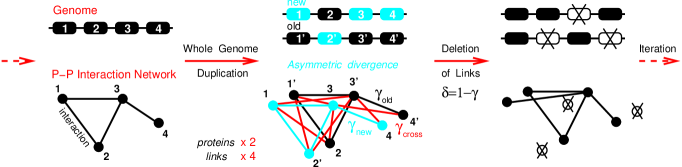
Figure 1: Model of protein-protein interaction network evolution through whole genome duplication. Whole genome duplications are followed by asymmetric divergence of protein duplicates with random distribution between genome copies (e.g. 1/$1^{\prime}$ vs 2/$2^{\prime}$): “New” duplicates are left essentially free to accumulate neutral mutations with the likely outcome to become nonfunctional and eventually deleted unless some “new”, duplication-derived interactions are selected; “Old” duplicates, on the other hand, are more constrained to conserve “old” interactions already present before duplication. The duplicated network with quadruplated links is graphically rearranged for convenience into old and new network copies (e.g. 2 and 2^′ duplicated nodes are swapped here). Links from the duplicated network are then kept with different probabilities $\gamma_{i}$ ($0\leq\gamma_{i}\leq 1$) reflecting this asymmetric divergence between protein duplicates. An alternative model based on symmetric divergence of protein duplicates and random link “complementation”vazquez ; middendorf is illustrated in Fig.S1 and discussed in the text.

Gene duplication is considered the main evolutionary source of new protein functionsli . Although long suspectedohno ; sparrow , whole genome duplications have only been recently confirmedsimillion ; kellis ; dujon ; jaillon ; dehal through large scale comparisons of complete genomeswong ; kellis .

Whole genome duplications are rare evolutionary transitions followed by random nonfunctionalization of most gene duplicates on time scales of about 100MY (with large variations between genes, see discussion). Whole genome duplications presumably provide unique opportunities to evolve many new functional genes at once through accretion of functional domainsdoolittle1 ; riley ; koonin ; apic ; orengo from contiguous pseudogenes (or redundant genes) and may also promote speciation events by preventing genetic recombinations between close descendants with different random deletion patterns.

Recent whole genome duplications (WGDs) within the last 500MY (about 15% of life history) have now been firmly established in all major eukaryote kingdoms. For instance, there are 4 consecutive WGDs between the seasquirt Ciona intestinalis and the common carp Cyprinus carpio, with most tetrapods (including mammals) in between at $+2$WGDs from seasquirt and $-2$WGDs from carp and most bony fish at $+3$WGDs from seasquirt and $-1$WGDs from carp (a pseudotetraploid bony fish duplicated about 10MY ago)panopoulou ; dehal ; jaillon ; david . There are also 3 consecutive WGDs in the recent evolution of the flowering plant Arabidopsis thalianasimillion and at least 3 consecutive WGDs for the protist Paramecium tetraurelia (Patrick Wincker, personal communication). Extrapolating these 500MY old records, one roughly expects a few tens consecutive WGDs (or equivalent “doubling events”) since the origin of life. These rare but dramatic evolutionary transitions must have had major consequences on the evolution of large biological networks, such as protein-protein interaction (PPI) networks.

From a theoretical point of view, we also expect that alternating whole genome duplications and extensive gene deletions lead to exponential dynamics of PPI network evolution. In the long time limit, this should outweigh all time-linear dynamics that have been assumed in PPI network evolution models under local structure changesalbert2001 ; barabasi ; raval ; vazquez ; berg ; ispolatov1 ; ispolatov2 (see discussion). In fact, the intrinsic exponential dynamics of genome evolution is already transparent from the wide distribution of genome sizesli ; sparrow and proliferation of repetitive elementshartl : it is hard to imagine that the $10^{4}$-fold span in lengths of eukaryote genomes could have solely arised through time-linear increases (and decreases) in genome sizes.*

Modelling PPI network evolution by whole genome duplication

We propose a simple model of PPI network evolution focussing on whole genome duplication (extensions to local or partial genome duplication are presented in refevlampiev_qbio and confirm the conclusions of this paper). Each time step $n$ corresponds to a whole genome duplication and leads to a complete duplication of the PPI network, whereby each node is duplicated ($\times 2$) and each interaction quadruplated ($\times 4$) as depicted on Fig.1. Links from the duplicated network are then kept with different probabilities $\gamma_{i}$ ($0\leq\gamma_{i}\leq 1$) reflecting symmetric or asymmetric divergences between protein or link copies.

The interaction network is caracterized at each step $n$ by its number of nodes with $k$ neighbours $N_{k}^{(n)}$ and its total number of links $L^{(n)}=\sum_{k\geq 1}kN_{k}^{(n)}/2$. As stochastic differences exist between network realizations, we study the evolution of typical networks by introducing a generating function averaged over all network realizations,

$$F^{(n)}(x)=\sum_{k\geq 0}\langle N_{k}^{(n)}\rangle x^{k}.$$ (1)

This use of generating functions can in fact be generalizedevlampiev_qbio to other, possibly non local features of interest (e.g. the average connectivity of first neighbors $g_{k}$maslov is introduced below).

In the following, we discuss a general model of PPI network evolution through whole genome duplication with asymmetric divergence of duplicated genes (Figs.1&2A). We compare it, first, to an alternative model with symmetric protein divergence but random link “complementation”vazquez ; middendorf (Fig.S1), and also to direct physical interactions from Yeast PPI network data (Fig. 2B&C). We then redefine this initial asymmetric divergence model (Fig. 1) in terms of protein-binding domains (Figs. 3A&B) to account for indirect protein-protein interaction within multi-protein complexes (Figs. 3A&C).

Asymmetric divergence of duplicated proteins

The case of asymmetric divergence between duplicated genes corresponds to the following evolution scenario; while duplicated proteins are initially equivalent and experience, at first, the same functional constraintskondrashov , their divergence becomes eventually asymmetriczhang ; conant ; gu (see discussion). This presumably occurs once one duplicate copy has lost an essential interaction and thus function, which has then to be fullfilled entirely by the other duplicate. The evolution of this latter duplicate is, from then on, more constrained to retain “old” interactions, while the former duplicate is left largely free to accumulate more neutral mutations with the likely outcome to become nonfunctional, unless some “new”, duplication-derived interactions are selected, Fig. 1 (new interactions arising from horizontal gene transfer are more characteristic of prokaryote evolutiondoolittle2 and neglected hereispolatov1 ). Note that “old” and “new” labels in Fig. 1 refer to the asymmetric conservation and fate of duplicates after WGD (and not to specific genome copies). Functionalization patterns of duplicated genes are further discussed in the supporting information.

The recurrence relation for the generating function (1) is derived as follows: since each node is initially duplicated, $F^{(n+1)}(x)$ is the sum of two $F^{(n)}(x)$ where $x$ is first replaced by $x^{2}$ (since each node degree can at most double) and then substituted as $x\rightarrow\gamma_{i}x\!+\!\delta_{i}$ where $\gamma_{i}$ [resp. $\delta_{i}=1-\gamma_{i}$] corresponds to the probability to keep [resp. delete] each link emerging from each node of the duplicated graph. Hence, the generating function recurrence for PPI network evolution with asymmetric divergence of duplicated proteins yields,

$$F^{(n+1)}(x)=F^{(n)}\bigl{(}(\gamma x\!+\!\delta)(\gamma_{\rm n}x\!+\!\delta_{\rm n})\bigr{)}+F^{(n)}\bigl{(}(\gamma x\!+\!\delta)(\gamma_{\rm o}x\!+\!\delta_{\rm o})\bigr{)}.$$ (2)

where $\gamma$, $\gamma_{\rm n}$ and $\gamma_{\rm o}$ [resp. $\delta$, $\delta_{\rm n}$ and $\delta_{\rm o}$] stand for $\gamma_{\rm cross}$, $\gamma_{\rm new}$ and $\gamma_{\rm old}$ [resp. $\delta_{\rm cross}$, $\delta_{\rm new}$ and $\delta_{\rm old}$] in Fig.1 (see supporting information for proof details).

The overall graph dynamics through successive global duplications is clearly exponential as anticipated; in particular, the total number of nodes grows as $F^{(n)}(1)=A\cdot 2^{n}$, where $A$ is the initial number of nodes, and the number of links scales as $\langle L^{(n)}\rangle\propto(2\gamma\!+\!\gamma_{\rm o}\!+\!\gamma_{\rm n})^{n}$. We remove permanently disconnected nodes from the list of relevant nodes, assuming that they correspond to proteins that have in fact lost their function and are eventually eliminated from the genome. To this end, we redefine the graph size as, $\langle N^{(n)}\rangle=\sum_{k\geq 1}\langle N_{k}^{(n)}\rangle$ and introduce a normalized generating function $p^{(n)}(x)$ for the mean degree distribution,

$$p^{(n)}(x)=\sum_{k\geq 1}p^{(n)}_{k}x^{k},{\rm~{}~{}~{}~{}where~{}~{}~{}~{}}p^{(n)}_{k}={\langle N_{k}^{(n)}\rangle\over\langle N^{(n)}\rangle}.$$ (3)

Absolute and relative generating functions are related through,

$$F^{(n)}(x)=p^{(n)}(x)\langle N^{(n)}\rangle+\langle N_{0}^{(n)}\rangle.$$ (4)

Inserting this expression (4) in recurrence (2) gives a closed relation between successive $p^{(n)}(x)$,

$$p^{(n+1)}(x)=1-$$ (5)

$${2-p^{(n)}\bigl{(}(\gamma x\!+\!\delta)(\gamma_{\rm n}x\!+\!\delta_{\rm n})\bigr{)}-p^{(n)}\bigl{(}(\gamma x\!+\!\delta)(\gamma_{\rm o}x\!+\!\delta_{\rm o})\bigr{)}\over\Delta^{(n)}},$$

where $\Delta^{(n)}$ is the ratio between consecutive numbers of connected nodes, $\Delta^{(n)}={\langle N^{(n+1)}\rangle/\langle N^{(n)}\rangle}=2-p^{(n)}(\delta\delta_{\rm n})-p^{(n)}(\delta\delta_{\rm o})\leq 2$.

The evolution of the mean degree is obtained by taking the first derivative of (5) at $x=1$:

$$\partial_{x}p^{(n+1)}(1)={\Gamma_{\rm n}\!+\!\Gamma_{\rm o}\over\Delta^{(n)}}\partial_{x}p^{(n)}(1),$$ (6)

where $\Gamma_{\rm n}=\gamma\!+\!\gamma_{\rm n}$ and $\Gamma_{\rm o}=\gamma\!+\!\gamma_{\rm o}$ hereafter.

We will limit the discussion here to degree distributions approaching a stationary regimes $p^{(n)}(x)\rightarrow p(x)$ with a finite mean degree $1\leq p^{\prime}(1)<\infty$. This seems to cover the most biologically relevant networks; for completeness, other cases are discussed elsewhereevlampiev_qbio . From (6) and the condition of finite mean degree, we readily obtain that $\Delta^{(n)}\rightarrow\Gamma_{\rm n}\!+\!\Gamma_{\rm o}$, which implies that the network evolution is asymptotically equivalent in terms of connected nodes and links,†

$${\langle N^{(n+1)}\rangle/\langle N^{(n)}\rangle}\rightarrow{\langle L^{(n+1)}\rangle/\langle L^{(n)}\rangle}=\Gamma_{\rm n}\!+\!\Gamma_{\rm o}\leq 2,$$ (7)

The stationary degree distribution is then solution of the functional equation,

$$p(x)=1-{2-p\bigl{(}(\gamma x\!+\!\delta)(\gamma_{\rm n}x\!+\!\delta_{\rm n})\bigr{)}-p\bigl{(}(\gamma x\!+\!\delta)(\gamma_{\rm o}x\!+\!\delta_{\rm o})\bigr{)}\over\Gamma_{\rm n}\!+\!\Gamma_{\rm o}},$$ (8)

which can be differentiated $k$ times to express the $k$th derivative in terms of lower derivatives,

$$\partial_{x}^{k}p(1)\left[1-{\Gamma_{\rm n}^{k}+\Gamma_{\rm o}^{k}\over\Gamma_{\rm n}+\Gamma_{\rm o}}\right]=\sum_{m=[k/2]}^{k}\alpha_{m}(\gamma_{\rm n},\gamma_{\rm o},\gamma)\partial_{x}^{m}p(1)$$ (9)

where the coefficients $\alpha_{m}$ are all positive from the definition (3).

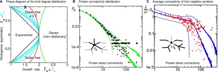
Figure 2: Analytical and numerical results of PPI Network evolution through whole genome duplication. A. Phase diagram for the limit degree distribution (see text). B&C. Comparison with protein direct physical interaction data for Yeast from BINDbind and MIPSmips databases: BIND (August 11, 2005 release), 4576 proteins, 9133 physical interactions, $\overline{k}=3.99$, $\overline{k^{2}}=106$ (filled symbols) and MIPS (downloaded online April 20, 2006), 4153 proteins, 7417 physical interactions, $\overline{k}=3.57$, $\overline{k^{2}}=78.6$ (open symbols). Squares correspond to raw data, while circles and triangles are statistically averaged with gaps in connectivity distribution for large $k\geq 20$, due to the finite size of Yeast PPI network. B. One-parameter fit of connectivity distribution data $p_{k}$ (corresponding to the “X” mark in A., see text). Numerical connectivity distribution averaged over 10,000 network realizations (central green line). Numerical averages plus or minus two standard deviations ($\pm 2\sigma$) are also displayed to show the predicted dispersions (upper and lower green lines) [Raw data (squares) do not fit within the mean $\pm 2\sigma$ curves for large $k$ due to the finite size of Yeast PPI network]. The fitting parameter $\gamma=0.26$ corresponds to an effective growth rate of $1+2\gamma=1.52$. C. One-parameter fit of average connectivity of first neighbor proteins $g_{k}$maslov (i.e. $k.g_{k}$ sums connectivities of first neighbors from proteins of connectivity $k$). Numerical predictions averaged over 10,000 network realizations (central blue line). Numerical averages plus or minus two standard deviations are also displayed (upper and lower blue lines). Same fitting parameter value as in B, $\gamma=0.26$. Note that $g_{k}$ is rescaled by $\overline{k}/\overline{k^{2}}$ (as $\overline{kg_{k}}=\overline{k^{2}}$ holds for each network realization); this rescales large $g_{k}$ fluctuations between network realizations, due to the divergence of $\overline{k^{2}}$ for $p_{k}\sim k^{-\alpha-1}$ with $2>\alpha>0$ for the one-parameter model.

The finite or infinite nature of $\partial_{x}^{k}p(1)$ depends on the two parameters $\Gamma_{\rm n}$ and $\Gamma_{\rm o}$ and defines the form of the limit degree distribution. The phase diagram Fig. 2A summarizes in the plane $(\Gamma_{\rm o}\!+\!\Gamma_{\rm n},\Gamma_{\rm o}\!-\!\Gamma_{\rm n})$ the different regimes for the asymptotic degree distribution $p_{k}$. $\Gamma_{\rm o}\!+\!\Gamma_{\rm n}$ is the global growth rate of the network ($\Gamma_{\rm o}\!+\!\Gamma_{\rm n}>1$ to ensure a growing network) and $\Gamma_{\rm o}\!-\!\Gamma_{\rm n}$ corresponds to the divergence asymmetry between duplicated proteins. We now discuss the two main stationary regimes for $p_{k}$ in the case of $\Gamma_{\rm n}\leq\Gamma_{\rm o}$ (the case $\Gamma_{\rm n}\geq\Gamma_{\rm o}$ is deduced by permutating indices):

$\bullet$ Exponential, non-conservative regime. If both $\Gamma_{\rm o}\!<\!1$ and $\Gamma_{\rm n}\!<\!1$,

$$\Gamma_{\rm n}^{k}+\Gamma_{\rm o}^{k}<\Gamma_{\rm n}+\Gamma_{\rm o},{\rm~{}~{}~{}~{}for~{}all~{}~{}}k\geq 2$$ (10)

and the factor in front of $\partial_{x}^{k}p(1)$ in (9) is always strictly positive, which implies that all derivatives of the limit degree distribution are finite. Hence, in this case, the limit degree distribution decreases more rapidly than any power law (see explicit asymptotic development inevlampiev_qbio ). Note that this “exponential” regime occurs when the links emerging from each node (Fig. 1) are more likely lost than duplicated at each round of global duplication (as $\Gamma_{\rm i}=\gamma\!+\!\gamma_{\rm i}<1$ is equivalent to $\delta\delta_{\rm i}>\gamma\gamma_{\rm i}$). This implies that most nodes eventually disappear, and with them all traces of network evolution, after just a few rounds of global duplication. The network topology is not conserved, but instead continuously renewed from duplication of the (few) most connected nodes.

$\bullet$ Scale-free, conservative regime. If $\Gamma_{\rm o}>1>\Gamma_{\rm n}$, the factor in front of $\partial_{x}^{k}p(1)$ in (9) can become negative. However, since the generating function should have all its derivatives positive, a negative value for one of them means that it simply does not exist. In fact, for $\Gamma_{\rm n}\ln\Gamma_{\rm n}\!+\!\Gamma_{\rm o}\ln\Gamma_{\rm o}\geq 0$ (red line in Fig.2A and evlampiev_qbio ), there is an integer $r\geq 1$ such that,

$$\Gamma_{\rm n}^{r}+\Gamma_{\rm o}^{r}\leq\Gamma_{\rm n}+\Gamma_{\rm o}<\Gamma_{\rm n}^{r+1}+\Gamma_{\rm o}^{r+1}.$$ (11)

implying that all derivatives $\partial_{x}^{k}p(1)$ are finite up to the $r$th order, while $\partial_{x}^{r+1}p(1)$ is infinite. This justifies the following asymptotic expansion of $p(x)$ in the vicinity of $x=1$,

$$p(x)=1-A_{1}(1-x)+\ldots+(-1)^{r}A_{r}(1-x)^{r}-A_{\alpha}(1-x)^{\alpha}-\ldots,$$ (12)

for some appropriate $r<\alpha<r+1$. This anzats is then inserted in (8) using $(\gamma x\!+\!\delta)(\gamma_{\rm n,o}x\!+\!\delta_{\rm n,o})=1-\Gamma_{\rm n,o}(1-x)\!+\!\gamma\gamma_{\rm n,o}(1-x)^{2}$ to obtain an equation on the coefficients $A_{1}$,… $A_{r}$. The term $A_{\alpha}$ does not mix with previous terms and gives the following equation for $\alpha$,

$$\Gamma_{\rm n}^{\alpha}+\Gamma_{\rm o}^{\alpha}=\Gamma_{\rm n}+\Gamma_{\rm o}.$$ (13)

The limit degree distribution follows a power law in this case,‡

$$p_{k}\propto k^{-\alpha-1},$$ (14)

(see red and blue “exponent” lines in Fig. 2A for $\alpha\!+\!1=2,3,4,\ldots$)

Note that scale-free degree distributions emerge under successive, global network duplications only if the “old” node copy has its links more likely duplicated than lost at each round of global duplication (as $\Gamma_{\rm o}=\gamma\!+\!\gamma_{\rm o}>1$ is equivalent to $\gamma\gamma_{\rm o}>\delta\delta_{\rm o}$). Thus, “old” nodes statistically keep on increasing their connectivity once they have emerged as “new” nodes by duplication. This implies that most nodes and their surrounding links are conserved throughout the evolution process, thereby ensuring that local topologies of previous networks remain embedded in subsequent networks.

In summary, whole genome duplication with asymmetric divergence of duplicated proteins leads to the emergence of two classes of PPI networks with finite asymptotic degree distributions : i) PPI networks with an exponential degree distribution and without conserved topology and ii) PPI networks with a scale-free limit degree distribution and at least local topology conservation. All other evolution scenarios, which do not lead to finite asymptotic degree distributions, are unlikely to model biologically relevant cases; they correspond either to an exponential disappearance of the whole PPI network (i.e. if $\Gamma_{\rm n}+\Gamma_{\rm o}<1$) or to an exponential shift of all proteins towards higher and higher connectivities (i.e. dense regime in Fig. 2A for $\Gamma_{\rm n}\Gamma_{\rm o}>1$)evlampiev_qbio .

Symmetric divergence of duplicates with link “complementation”

Another model of interest is the so-called “duplication-mutation-complementation” model initially proposed in the context of protein network evolution through successive local duplicationsvazquez ; middendorf . This model can be easily adapted to the context of PPI network evolution through whole genome duplication, Fig. S1. After each global duplication step, the probability to keep an instance of each interaction is now distributed randomly over the four equivalent links without reference to particular protein duplicates, unlike in the previous model. The complementation step (which ensures that at least one instance of each previous link is retained) can be enforced here through the “old” link copy ($\gamma_{\rm o}=1$) with $\gamma_{\rm n}$ corresponding to the “new” interaction sharing no node with $\gamma_{\rm o}$, while $\gamma$ still pertains to the last two equivalent cross links. This model is thus effectively symmetric from the protein point of view and readily yields the following recurrence for the generating function of the network degree distribution.

$$F^{(n+1)}(x)=2F^{(n)}\bigl{(}(\gamma x\!+\!\delta)({\gamma_{\rm e}}x\!+\!{\delta_{\rm e}})\bigr{)},$$ (15)

where $\gamma_{\rm e}=(\gamma_{\rm n}\!+\!\gamma_{\rm o})/2$ and $\delta_{\rm e}=(\delta_{\rm n}\!+\!\delta_{\rm o})/2$ are effective average probabilities to retain or delete old and new links (see supporting information for proof details). Hence, the model of PPI network evolution with link complementation is in fact equivalent to the case of a symmetric divergence of duplicated proteins in the previous general model. Such symmetric divergence of duplicated proteins yields either a stationary exponential regime ($\Gamma_{\rm n}+\Gamma_{\rm o}<2$, Fig.2A) or a non-stationary dense regimeevlampiev_qbio ($\Gamma_{\rm n}+\Gamma_{\rm o}>2$, Fig.2A).

Hence, the “duplication-mutation-complementation” model cannot lead to scale-free degree distributions, and thus to locally conserved network topology, in the context of whole genome duplication evolution, by contrast to the same model applied to local duplication with time-linear evolutionvazquez ; middendorf .

Fitting PPI network data with a one-parameter model

Scale-free degree distributions have been widely reported for large biological networks and other exponentially growing networks like the WWW. We showed in the previous discussion that scale-free limit degree distributions require an asymmetric divergence of duplicated proteins ($\Gamma_{\rm o}-\Gamma_{\rm n}=\gamma_{\rm o}-\gamma_{\rm n}>0$) which corresponds to the probability difference between conservation of old interactions ($\gamma_{\rm o}$) and coevolution of new binding sites ($\gamma_{\rm n}$). The expected range of parameters for actual biological networks is $1\simeq\gamma_{\rm o}\gg\gamma\gg\gamma_{\rm n}\simeq 0$; In particular, the most conservative ($\gamma_{\rm o}=1$) and least correlated ($\gamma_{\rm n}=0$) evolution scenario corresponds to the strongest divergence asymmetry between duplicated proteins ($\Gamma_{\rm o}-\Gamma_{\rm n}=1$, upper border on Fig.2A). The condition $\gamma_{\rm o}=1$ ensures that not only local but also global topologies of all previous networks remain embedded in all subsequent networks. This model is effectively a one-parameter model ($\gamma$) for PPI network evolution through whole genome duplication. It converges towards a stationary scale-free limit degree distribution $p_{k}\sim k^{-\alpha-1}$ with $0<\alpha<2$ for $0<\gamma<(\sqrt{5}-1)/2$ and generates non-stationary dense networks for $(\sqrt{5}-1)/2<\gamma<1$evlampiev_qbio . We used this one-parameter model to fit both the degree distribution (Fig.2B) and the average connectivity of first neighbors (Fig.2C) for direct physical interaction data of S. cerevisiae taken from two databases, BINDbind and hand curated MIPSmips (with presumabky fewer nonspecific spurious interactionsdeeds ). The predicted asymptotic regime is in fact approached for $k\leq 20$ due to the finite size of Yeast PPI network. The fitting parameter $\gamma=0.26$ corresponds to a fixed growth rate (7) of $1+2\gamma=1.52$ (i.e. the number of links and nodes increases by 52% at each global duplication). Adding and removing up to 30% of links randomly, or drawing $\gamma$ from a uniform distribution between 0 and 0.52 (with average $\bar{\gamma}=0.26$) yield remarkably similar fits (not shown) to the experimental data. This reveals a large insensibility to false- positive and negative noises and fluctuations in $\gamma$ (as long as the non-stationary dense regime is avoided, Fig.2A). The fixed (or averaged) growth rate of 52% at each round of global duplication is enough to generate networks of the size of S. cerevisiae starting from a few interacting “seeds” after about 20 global duplications (i.e. $1.52^{20}=4334$ times more nodes with an average of one global duplication per 200MY for 4BY). Such scenario is not a priori incompatible with experimental data, as we only have clear records on global duplications dating back up to 400-500MY ago (i.e. only 10 to 20% of life history). Yet, these records suggest that “recent” whole genome duplications might be more frequent (every 100-150MY) and more selective (growth rates between 10 and 25%).§

Direct vs indirect protein-protein interactions

The protein-protein interactions we have considered so far correspond to direct physical contact between protein pairs derived, for instance, from two-hybrid expression assaysfields . However, we expect from the proposed scale-free fit of the degree distribution (Fig. 2B) that the underlying PPI network has conserved not only pairwise interactions during evolution but also some level of network topology (see above). The emergence of locally conserved topology in PPI network evolution leads “naturally” to conserved associations or “modules” between multiple proteinsdokholyan ; spirin ; wuchty2003 ; wuchty2004 ; vergassola and, beyond, to recurrent “motifs” across different types of biological networkshartwell ; milo2002 ; guelzim ; yeger-lotem2004 ; francois ; berg2 ; mazurie ; buchler2005 .

In fact, many biological functions are known to rely on multiple direct and indirect interactions within protein complexes. Moreover, the combinatorial complexity of multiple-protein interactions is likely responsible for the remarkable diversity amongst living organismsbirchler , despite their rather limited and largely shared genetic background (i.e. a few (ten) thousands genes built from a few hundreds families of homologous protein domainsmurzin ; apic ; superfamilly ; orengo ).

High-throughput studies using affinity precipitation methods coupled to mass spectroscopygavin2002 ; ho2002 ; gavin2006 have proposed some 80,000 direct and indirect protein interactions for S. cerevisiae (raw data) and similar data are now becoming available for several other species.

Yet, from a theoretical point of view, the evolution of indirect interactions is expected to depend not only on locally conserved network topology but also on the actual “combinatorial logic” between direct interactions. This cannot be readily defined on traditional PPI network representation (e.g. Fig. 1) and requires a somewhat more elaborate model as we now discuss.

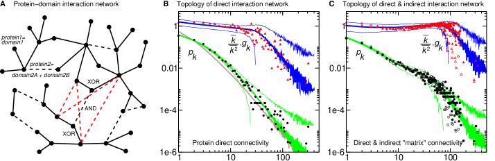
Figure 3: Combining whole genome duplication and domain shuffling of multi-domain proteins.
A. Protein-domain interaction network. Nodes now correspond to single binding domains in a protein-domain interaction network (solid lines). Multi-binding-domain proteins are introduced through a new type of links corresponding to covalent peptide bonds between protein domains (black dashed lines). This provides a graphical framework to distinguish mutually exclusive, direct interactions (“XOR”) between protein domains from cummulative, indirect interactions (“AND”) within multi-protein complexes (red dashed lines). B&C. Comparison with protein direct & indirect interaction data for Yeast from BINDbind database (B&C filled symbols, indirect interactions fromho2002 ; gavin2002 ) and Refgavin2006 (C open symbols, see supporting information). Data are statistically averaged as in Fig. 2B&C to account for gaps in connectivities for large $k\geq 20$, due to the finite size of Yeast PPI network. B. Two-parameter fit of both direct connectivity distribution $p_{k}$ and average direct connectivity of first neighbor proteins $g_{k}$maslov (see Fig.2C and text). Numerical predictions are averaged over 1,000 network realizations (central green and blue lines). Numerical averages plus or minus two standard deviations are also displayed to show the predicted dispersions (upper and lower green and blue lines). The two adjusted parameters ($\gamma=0.1$ and $\lambda=0.3$) correspond to a network growth rate of 20% and an average of 1.5 protein-binding sites (domains) per protein. The connectivity distribution of the underlying single-domain network (corresponding to $\gamma=0.1$ and $\lambda=0.0$) is also displayed (brown line) to illustrate its relation to the full multi-domain protein network (see text). C. Two-parameter fit of both direct & indirect “matrix” connectivity distribution $p_{k}$ and average direct & indirect “matrix” connectivity of first neighbor proteins $g_{k}$maslov (see text). Same two adjusted parameters ($\gamma=0.1$ and $\lambda=0.3$) as in B while a selection of indirect interactions is added up to a total of 28,000 direct & indirect interactions (see supporting information).

Redefining PPI network evolution in terms of protein domains

Indirect protein interactions reflect the occurence of simultaneous direct interactions within protein complexes. This requires that some proteins have more than one binding sites to simultenaously interact with several protein partners. Indeed, proteins with a single protein-binding site can only bind to one partners at a time, underlying a simple “XOR”-like combinatorial logic. By contrast, proteins with several protein-binding sites (which are usually multi-domain proteins) greatly increase the combinatorial complexity of biological processes (like gene regulation or cell signaling) by adding “AND” operators to the computational logic between multiple direct interactions. Multi-domain proteins also provide a versatile support for protein evolution through accretion or deletion of individual domainsdoolittle1 ; riley ; koonin ; apic ; orengo .

In addition, we note that binding sitessheinerman ; levy on specific protein domains are likely the primary source of asymmetric divergence in PPI network evolution, as binding site mutations necessarily affect interactions with all binding partners (Fig. 1) and not just a random subset of them (Fig. S1). Hence, asymmetric divergence of protein duplicates “naturally” originates from “spontaneous symmetry breaking” of their equivalent protein-binding sites (or domains).

We propose to highlight this central role of protein domains in the evolution of PPI networks by simply redefining our initial asymmetric divergence model (Fig. 1) in terms of protein-binding domains (i.e. with a single protein-binding site) as illustrated in Fig. 3A. This alternative representation of PPI networks provides a theoretical framework to model the evolution of the combinatorial logic underlying PPI networks, as it distinguishes mutually exclusive, direct interactions (“XOR”) between protein domains (Fig.3A, black solid lines) from cummulative, indirect interactions (“AND”) within multi-protein complexes (Fig.3A, red dashed lines).

Combining whole genome duplication and domain shuffling.

As noted in the introduction, whole-genome duplications promote efficient shuffling of multi-domain proteins by enabling many accretion and deletion events of functional domains after each genome doubling. We will assume in the following that this shuffling of multi-domain proteins is so efficient that protein domains encoded along the genome evolve independently from their inclusion in single- or multi-domain proteins (indeed, different multi-domain combinations are typically observed across living kingdomsorengo ). Besides, a more elaborate model of protein evolution detailing domain accretion and deletion events leads to virtually identical results for the large scale topological features of PPI network (not shown). The asymptotic generating function $\tilde{p}(x)$ for multi-domain protein networks with independent domain evolution can be deduced a posteriori as,

$$\tilde{p}(x)\!=\!(1-\lambda)p(x)\bigl{(}1+\lambda p(x)+\lambda^{2}p^{2}(x)+\ldots\bigr{)}\!=\!{(1-\lambda)p(x)\over 1-\lambda p(x)}$$

where $\lambda$ is the probability of covalent connection between successive protein domains encoded along the genome. This leads to an exponential distribution of multi-domain proteins, in agreement with actual distributionswolf ; ekman , with an average of $1/(1-\lambda)$ protein-binding sites per protein. While $p(x)$ now reflects the independent evolution of single protein-binding domains according to Eqs.(8,12), it also controls the asymptotic properties of the derived multi-domain networks $\tilde{p}(x)$; in particular, for $\Gamma_{\rm o}>1>\Gamma_{\rm n}$, we obtain from Eq.(12) the following asymptotic expansion in the vicinity of $x=1$,

$$\tilde{p}(x)=1-{1-p(x)\over 1-\lambda p(x)}\sim 1-\ldots-{A_{\alpha}\over 1-\lambda}(1-x)^{\alpha}-\ldots$$

which implies that degree distributions of multi-domain protein networks $\tilde{p}_{k}$ increase with respect to the underlying single-domain interaction network $p_{k}$ as $\tilde{p}_{k}\sim p_{k}/(1-\lambda)$ for large $k$, while the fraction of proteins with a single binding partner $\tilde{p}_{1}$ decreases at the same time as $\tilde{p}_{1}=\tilde{p}^{\prime}(0)=(1-\lambda)p^{\prime}(0)=(1-\lambda)p_{1}$ (see Fig. 3B). Note that the scale-free degree distribution of such multi-domain protein networks results from an asymmetric divergence of individual binding sites (or domains) rather than asymmetric divergence of global protein architectures. This has also consequences for the functionalization of duplicated genes (see supporting information). In particular, random (symmetric) “subfunctionalization” between protein duplicates at the level of protein domains does not prevent the emergence of scale-free networks with locally conserved topology, by contrast to random link “complementation” at the level of individual interactions (Fig. S1) which leads to exponential networks without conserved topology (as discussed above).

Hence, domain shuffling of multi-domain proteins provides a powerful, yet non-disruptive source of combinatorial innovation, as it preserves essential topological features inherited from the underlying protein-domain interaction network evolution.

Finally, comparison with experimental data sets including indirect protein-protein interactionsgavin2002 ; ho2002 ; gavin2006 is made by adopting a statistical implementation of the “combinatorial logic” discussed above (see supporting information). It is based on a Dijkstra algorithm that estimates the relative importance of all possible indirect interactions between multi-domain (and single-domain) proteins for each PPI network realization. Figs. 3B&C show rather good fits of experimental data sets corresponding to an estimated 30% to 60% coverage of actual PPI networksgavin2002 ; ho2002 ; gavin2006 (see, however, supporting information). The two adjusted parameters, $\gamma=0.1$ and $\lambda=0.3$, correspond to a network growth rate of 20% (i.e. $1+2\gamma$) and an average of 1.5 (i.e. $1/(1-\lambda)$) protein-binding sites (domains) per protein in agreement with broad estimates for these biological parameters (see above §  and wolf ; ekman ). This also confirms that the properties of PPI networks we have predicted from first principles (i.e. i) exponential dynamics and ii) symmetry breaking) are already transparent from partial data sets.

Discussion

Beyond whole genome duplications, local genome rearrangements such as small segmental duplications, rearrangements and horizontal transfers might well have been critical for the emergence and proliferation of living organisms. Moreover, we note that local duplications/deletions may also lead to exponential dynamics of PPI network evolution if they are selected independently in parallel (exponential models of local or partial genome duplication are presented in refevlampiev_qbio ). Yet, recent records ($<$500MY) from various eukaryote kingdoms (from protists to animals and plants) suggest that the majority of duplicates may still have arised from successive whole genome duplications (although this will need to be confirmed as more fully sequenced eukaryote genomes will become available).

One possible origin for this less efficient selection of local duplications might be the dosage imbalance they initially induce, thereby raising the odds for their rapid nonfunctionalizationfraser ; papp ; maere (unless proved beneficial under concomitant environmental changeskondrashov ). By contrast, rapid nonfunctionalization of duplicates following a whole genome duplication should be opposed by dosage effect. This is because whole genome duplications initially preserve correct relative dosage between expressed genes, while subsequent random nonfunctionalizations disrupt this initial dosage balance. Preventing rapid asymmetric divergence between duplicates from recent whole genome duplications appears, in the end, to increase their chance of neo- or subfunctionalization by favoring longer (symmetric) genetic drift rather than early (asymmetric) functional loss.

Conclusion

Large scale topological features of PPI networks emerge “spontaneously” in the course of evolution under simple duplication/deletion eventsispolatov1 , regardless of the specific evolutionary advantages individual proteins might have been selected for. Yet, the intrinsic exponential dynamics of PPI network evolution by whole genome duplications (or independent local duplications selected in parallelevlampiev_qbio ) requires an asymmetric divergence of protein duplicates. Such asymmetric divergence arises “naturally” at the level of protein-binding sites or domains (through “spontaneous symmetry breaking”) and is robust to extensive domain shuffling of multi-domain proteins.

Acknowledgements. We thank U. Alon, M. Consentino-Lagomarsino, T. Fink, R. Monasson, M. Vergassola and C. Wiggins for discussion. This work was supported by CNRS, Institut Curie and HFSP.

Correspondence: herve.isambert@curie.fr

SUPPORTING INFORMATION

I.   Supplementary Figure.

FIG. S1: Alternative Model of PPI network evolution through whole genome duplication with symmetric divergence of duplicated proteins and random link “complementation”vazquez ; middendorf .

II.   Proof of Recurrence Relations for Generating Functions (Eq.2 and Eq.15).

After each whole genome duplication, each node has at most doubled its number of neighbors counted through powers of $x$ in the generating function. Hence, a given PPI network realization with $N_{k}$ nodes of connectivity $k$ ($k\geq 0$) will contribute to the next duplicated ensemble of PPI networks as,

$$N_{k}x^{k}\rightarrow N_{k}x^{2k}$$ (16)

After link deletion with probability $\delta$ or $\delta_{i}=\delta_{o},\delta_{n}$, it contributes to the $x^{m}$ terms of the generating function (with $m=0,\ldots,2k$) as,

$$N_{k}x^{2k}\rightarrow N_{k}\left(\sum_{\ell=0}^{k}\Big{(}{\begin{array}[]{*{20}c}k\\ \ell\\ \end{array}}\Big{)}(\gamma x)^{\ell}\delta^{k-\ell}\right)\left(\sum_{\ell=0}^{k}\Big{(}{\begin{array}[]{*{20}c}k\\ \ell\\ \end{array}}\Big{)}(\gamma_{i}x)^{\ell}\delta_{i}^{k-\ell}\right)=N_{k}\Big{(}(\gamma x+\delta)(\gamma_{i}x+\delta_{i})\Big{)}^{k}$$ (17)

for the asymmetric divergence model (Fig. 1, Eq. 2) and as,

$$N_{k}x^{2k} \rightarrow N_{k}\left(\sum_{\ell=0}^{k}\Big{(}{\begin{array}[]{*{20}c}k\\ \ell\\ \end{array}}\Big{)}(\gamma x)^{\ell}\delta^{k-\ell}\right)\left[\sum_{j=0}^{k}\Big{(}{\begin{array}[]{*{20}c}k\\ j\\ \end{array}}\Big{)}\left(\sum_{\ell_{o}=0}^{j}{1\over 2^{j}}\Big{(}{\begin{array}[]{*{20}c}j\\ \ell_{o}\\ \end{array}}\Big{)}(\gamma_{o}x)^{\ell_{o}}\delta_{o}^{j-\ell_{o}}\right)\left(\sum_{\ell_{n}=0}^{k-j}{1\over 2^{k-j}}\Big{(}{\begin{array}[]{*{20}c}k-j\\ \ell_{n}\\ \end{array}}\Big{)}(\gamma_{n}x)^{\ell_{n}}\delta_{n}^{k-j-\ell_{n}}\right)\right]$$ (26)

$$\rightarrow N_{k}\Big{(}(\gamma x+\delta)({\gamma_{e}}x+{\delta_{e}})\Big{)}^{k}$$ (27)

with $\gamma_{e}=(\gamma_{o}+\gamma_{n})/2$ and $\delta_{e}=(\delta_{o}+\delta_{n})/2$ for the symmetric divergence model with link “complementation”vazquez ; middendorf (Fig. S1, Eq. 15).

III.   Gene functionalization patterns in different models of PPI network evolution through whole genome duplication.

The initial model depicted on Fig. 1 with asymmetric divergence of duplicated proteins leads typically to “neofunctionalization” of “new” duplicates, while “old” duplicates retain most initial interactions (if not all for $\gamma_{o}=1$).

By contrast, the alternative model depicted on Fig. S1 with symmetric divergence of duplicated proteins and random link “complementation”vazquez ; middendorf leads typically to random “subfunctionalization” between protein duplicates at the level of individual interactions. However, this eventually leads to exponential degree distributions with no topology conservation of the PPI network (see main text), whereas scale-free degree distributions with at least local topology conservation of the PPI network indeed emerge under the initial asymmetric model, Fig. 1.

Yet, as discussed in the main text, the necessary asymmetric divergence of protein duplicates occurs “spontaneously” at the level of protein-binding sites rather than of the entire (multi-domain) proteins, as assumed in Fig. 1. This motivates the redefinition of the initial model in terms of protein-binding domains (Fig. 3A) to capture the asymmetric divergence of protein duplicates at the level of protein-binding sites and allow, at the same time, for extensive domain shuffling events of multidomain proteins (see main text).

This more elaborate model of PPI network evolution by whole genome duplication and domain shuffling encompasses both “neofunctionalization” and “subfunctionalization” of gene duplicates at the level of protein domains, in agreement with the suggestion that gene/protein evolution should be analyzed in terms of domains rather than entire proteinsdoolittle1 ; riley ; koonin ; apic ; orengo . In addition, this combined model of PPI network evolution also provides a theoretical framework to describe the evolution of the “combinatorial logic” behind indirect interactions within multi-protein complexes (see Fig. 3A and main text).

IV.   Statistical weighting of indirect interactions from protein complexes.

We use a statistical implemention of the “combinatorial logic” underlying indirect protein interactions. Indirect interactions between protein pairs are weighted by the product of binding site “availabilities” along the shortest weighted path of intermediate direct interactions connecting them. The “availability” $a_{i}$ of a binding site $i$ is defined as the relative expression level ($e_{i}$) with respect to its first neighbor binding partners $j$ of connectivity $d_{j}$,

$$a_{i}={e_{i}\over e_{i}+\sum_{j\in\langle i\rangle}e_{j}/d_{j}}<1$$ (28)

Where expression level $e_{j}$ can be distributed with specific statistics, such as randomly, uniformly or according to characteristic power laws, as reported experimentallyfraser ; krylov ; ueda ; lemos1 ; lemos2 . Yet, in practice, we found that the predicted large scale topological features of PPI networks depend only weakly on the specific distribution of expression levels (for reasonable distribution range).

The statistical probability of an (intermediate) direct interaction between domains $i$ and $j$ is then proportional to $a_{i}a_{j}$, which we use in a Dijkstra-like algorithmdijkstra for additive distance minimization assigning $d^{\circ}_{ij}=-\ln(a_{i}a_{j})>0$ weights between interacting domains $i$ and $j$. Because of the presence of both covalent peptide bonds and direct, noncovalent interactions between protein domains (Fig. 3A), indirect protein-protein interactions correspond to alternating paths of noncovalent and covalent interactions with no successive noncovalent interactions which are forbidden by the shared binding site constraint (i.e. a binding site can only interact with one binding partner at a time). We describe below an algorithm which performs a simultaneous minimization for paths starting with a covalent bond ($c_{ij}$) and paths starting with a direct, noncovalent interaction ($d_{ij}$). (An additional variable for second node $v_{ij}$ on the path is also needed to avoid non-physical “covalent loops”.)

The initialization of distances between protein domains is:

$$c^{\circ}_{ij}={\rm Max,}\;\;\;v^{\circ}_{ij}=j{\rm~{}~{}~{}~{}~{}~{}~{}~{}for~{}all~{}}(i,j){\rm~{}pairs,~{}and}$$

$$\delta_{ij}=d^{\circ}_{ij}\!=\!-\ln(a_{i}a_{j}){\rm~{}~{}~{}~{}~{}~{}for~{}direct,~{}noncovalent~{}interactions,}$$

$$\delta_{ij}=0,\;\;d^{\circ}_{ij}={\rm Max}{\rm~{}~{}~{}~{}~{}~{}~{}~{}for~{}covalent~{}bonds,}$$

$$\delta_{ij}=d^{\circ}_{ij}={\rm Max}{\rm~{}~{}~{}~{}~{}~{}~{}~{}~{}~{}~{}~{}~{}~{}otherwise.}$$

We then iterate until convergence (after $N^{2}\times$ (longest path) operations):

$$d^{\prime}_{ij}=\min\bigl{(}d_{ij},{\min_{k\in\langle i\rangle_{d}}(\delta_{ik}+c_{kj})}\bigr{)}$$

$$c^{\prime}_{ij}=\min\bigl{(}c_{ij},{\min_{k\in\langle i\rangle_{c},v_{kj}\neq i}(\delta_{ik}+\min(d_{kj},c_{kj}))}\bigr{)}$$

$$v^{\prime}_{ij}=\{k\in\langle i\rangle_{c}\;|\;v_{kj}\neq i,\;{\min(\delta_{ik}+\min(d_{kj},c_{kj}))}\}\;\;\;\;\;\;\;\;\;\;\;\;\;\;$$

and remove eventually the minimum paths starting with a covalent bond (to avoid double counting of indirect interactions for multidomain proteins below):

$$d_{ij}={\rm Max}{\rm~{}~{}~{}~{}~{}~{}~{}~{}~{}~{}~{}~{}~{}~{}~{}~{}~{}~{}~{}~{}~{}~{}~{}~{}if~{}~{}}d_{ij}\geq\min(c_{ij},c_{ji}){\rm~{}~{}~{}~{}~{}~{}~{}~{}~{}~{}~{}~{}~{}~{}}$$

Hence, the probabilities to observe a single indirect interactions within protein complexes is given by:

$$w_{ij}=0{\rm~{}~{}~{}~{}~{}~{}~{}~{}~{}~{}~{}~{}~{}~{}~{}~{}~{}~{}~{}~{}~{}~{}~{}~{}~{}~{}~{}~{}~{}~{}if~{}~{}~{}}d_{ij}={\rm Max}{\rm~{}~{}~{}~{}~{}~{}~{}~{}~{}~{}~{}~{}~{}~{}~{}~{}~{}~{}~{}~{}~{}~{}}$$

$$w_{ij}={\beta\exp(-d_{ij})}{\rm~{}~{}~{}~{}~{}~{}~{}~{}~{}~{}~{}~{}otherwise,~{}~{}~{}~{}~{}~{}~{}~{}~{}~{}~{}~{}~{}~{}~{}~{}~{}~{}~{}~{}~{}~{}~{}~{}~{}~{}~{}~{}~{}~{}~{}~{}~{}~{}~{}~{}~{}~{}~{}~{}~{}~{}~{}~{}~{}~{}~{}~{}~{}~{}~{}~{}~{}~{}~{}~{}~{}~{}~{}~{}~{}~{}~{}~{}~{}~{}~{}~{}~{}~{}~{}}$$

with the normalization condition $\Sigma_{i<j}w_{ij}=1$, which gives $1/\beta=\Sigma_{i<j}\exp(-d_{ij})$.
$w_{ij}$ is thus the normalized product of availabilities $a_{k}$ along the shortest weighted path between $i$ and $j$.

Finally, the individual probabilities $p_{ij}$ to observe a total of $M$ indirect interactions within protein complexes are given by:

$$p_{ij}=1-(1-w_{ij})^{n}{\rm~{}~{}~{}~{}~{}~{}~{}~{}~{}~{}~{}~{}~{}~{}~{}~{}~{}~{}~{}~{}~{}~{}~{}~{}~{}~{}~{}~{}~{}~{}~{}~{}~{}~{}~{}~{}~{}~{}~{}~{}~{}~{}~{}~{}~{}~{}~{}~{}~{}~{}~{}~{}~{}~{}~{}~{}}$$ (29)

where $n$ is solution of $\Sigma_{i<j}p_{ij}=M$.

Given the number $M$ of indirect interactions in various data setsgavin2002 ; ho2002 ; gavin2006 , we have assessed their expected contribution to the large scale topology of Yeast PPI network from the two-parameter $\gamma-\lambda$ model described in the main text. $M\simeq 28,000$ corresponds to the sum of about $9,000$ direct physical interactions from the BIND databasebind (Fig. 2B&C filled symbols) and about $19,000$ “matrix” interactions from ho2002 ; gavin2002 between $2,100$ proteins already involved in direct physical interactions (out of $4,576$ proteins in the BIND database, Fig. 3C filled symbols). “Matrix” interactions from ref.gavin2006 (Fig. 3C open symbols) are “reconstructed” from supplementary information files ofgavin2006 as follows: “matrix” interactions are included for (each complex core)$\times$(each associated “module”) and (each complex core)$\times$(each associated “attachment” = one protein). This reconstructed dataset should therefore be considered as incomplete, since “matrix” interactions between compatible modules and/or attachments associated to a given core are not taken into account (information not given ingavin2006 ).

Numerical fits ($\gamma=0.1$, $\lambda=0.3$) are displayed on Fig. 3C (for direct and indirect interactions) for both connectivity distribution (green) and average connectivity of first neighbors (blue). They corresponds to the same adjusted values ($\gamma=0.1$, $\lambda=0.3$) as in Fig. 3B (for direct interactions only).

References

- (1)
- (2)
- (3) Li, W.H. (1997) Molecular Evolution (Sinauer, Sunderland, MA).
- (4) Ohno, S. (1970) Evolution by Gene Duplication (Springer, New York).
- (5) Sparrow, A.H., & Naumann, A.F. (1976) Science, 192 524.
- (6) Simillion, C. et al. (2002) Proc. Natl. Acad. Sci. USA 99, 13627-13632.
- (7) Kellis, M., Birren, B.W., & Lander, E.S. (2004) Nature 428, 617-624.
- (8) Dujon, B., et al. (2004) Nature 430, 35-44.
- (9) Jaillon O., et al. (2004) Nature 431, 946-957.
- (10) Dehal, P., & Boore J.L. (2005) PLoS Biol. 3, e314.
- (11) Wong, S., Butler, G., & Wolfe, K.H. (2002) Proc. Natl. Acad. Sci. USA 99, 9272-9277.
- (12) Doolittle, R.F. (1995) Annu. Rev. Biochem. 64, 287-314.
- (13) Riley, M., & Labedan, B. (1997) J. Mol. Biol. 268, 857-868.
- (14) Koonin, E.V., Aravind, L., & Kondrashov, A.S. (2000) Cell 101, 573.
- (15) Apic, G., Gough, J., Teichmann, S.A. (2001) J. Mol. Biol. 310, 311-325.
- (16) Orengo, C.A., & Thornton, J.M. (2005) Annu. Rev. Biochem. 74, 867.
- (17) Panopoulou, G., et al. (2003) Genome Res. 13, 1056-1566.
- (18) David, L., Blum, S., Feldman, M.W., Lavi, U., & Hillel, J. (2003) Mol Biol Evol. 20, 1425-1434.
- (19) Albert, R., & Barabási, A.-L., (2001) Rev. Mod. Phys. 74, 47.
- (20) Raval, A. (2003) Phys Rev E Stat Nonlin Soft Matter Phys. 68, 066119.
- (21) Vázquez, A., Flammini, A., Maritan, A., & Vespignani, A. (2003) ComPlexUs 1, 38-44.
- (22) Barabási, A.-L., & Oltvai, Z.N., (2004) Nat. Rev. Genetics 5, 101.
- (23) Berg, J., Lässig, M., & Wagner, A. (2004) BMC Evol. Biol. 4, 51.
- (24) Ispolatov, I., Krapivsky, P.L., & Yuryev, A. (2005) Phys Rev E Stat Nonlin Soft Matter Phys. 71, 061911.
- (25) Ispolatov, I., Yuryev, A., Mazo, I., & Maslov, S. (2005) Nucleic Acids Res. 33, 3629-3635.
- (26) Hartl, D.L. (2000) Nat. Rev. Genet. 1, 147.
- (27) Evlampiev, K., & Isambert, H. (2006) to be submitted.
- (28) Maslov, S., & Sneppen, K. (2002) Science 296, 910.
- (29) Middendorf, M., Ziv, E., & Wiggins, C. (2005) Proc. Natl. Acad. Sci. USA 102, 3192-3198.
- (30) Kondrashov, F.A., Rogozin, I.B., Wolf, Y.I., & Koonin, E.V. (2002) Genome Biol. 3, research0008.1-research0008.9.
- (31) Zhang, P., Gu, Z. & Li, W.-H. (2003) Genome Biol. 4, R56.
- (32) Conant, G.C., & Wagner, A. (2003) Genome Res. 13, 2052-2058.
- (33) Gu, X., Zhang, Z., & Huang, W. (2005) Proc. Natl. Acad. Sci. USA 102, 707-712.
- (34) Doolittle, R.F. (2005) Curr. Opin. Struct. Biol. 15, 248-253.
- (35) Alfarano, C., et al. (2005) Nucl Acids Res. 33(suppl1), D418-D424.
- (36) Mewes, H.W., et al. (2006) Nucl Acids Res. 34(suppl1), D169-D17.
- (37) Deeds, E.J., Ashenberg, O., & Shakhnovich, E.I. Proc. Natl. Acad. Sci. USA 103, 311-316.
- (38) Uetz, P., et al. (2000) Nature 403, 623-627.
- (39) Dokholyan, N.V., Shakhnovich, B., & Shakhnovich, E.I. (2002) Proc. Natl. Acad. Sci. USA 99, 14132-14136.
- (40) Spirin V., & Mirny, L.A. (2003) Proc. Natl. Acad. Sci. USA 100, 12123.
- (41) Wuchty, S., Oltvai, Z.N., & Barabási, A.L. (2003) Nat. Genet. 35, 176.
- (42) Wuchty, S. (2004) Genome Res. 14(7), 1310-1314.
- (43) Vergassola, M., Vespignani, A., & Dujon, B. (2005) Proteomics 5, 3116-3119.
- (44) Hartwell, L.H., Hopfield, J.J., Leibler, S. & Murray, A.W. (1999) Nature 402, C47-C51.
- (45) Milo, R., et al. (2002) Science 298, 824.
- (46) Guelzim, N., Bottani, S., Bourgine, P., & Képès, F. (2002) Nat. Genet. 31, 60-63.
- (47) Yeger-Lotem E, et al. (2004) Proc. Natl. Acad. Sci. USA 101, 5934.
- (48) Francois, P., & Hakim, V. (2004) Proc. Natl. Acad. Sci. USA 101, 580.
- (49) Berg J., & Lässig, M. (2004) Proc. Natl. Acad. Sci. USA 101, 14689.
- (50) Mazurie, A., Bottani, S., & Vergassola, M. (2005) Genome Biol. 6, R35.
- (51) Buchler, N.E., Gerland, U., & Hwa, T. (2005) Proc. Natl. Acad. Sci. USA 102, 9559-9564.
- (52) Birchler, J.A., Bhadra, U., Bhadra, M.P., & Auger, D.L. (2001) Dev. Biol. 234, 275-288.
- (53) Murzin, A.G., Brenner, S.E., Hubbard, T., & Chothia, C. (1995) J. Mol. Biol. 247, 536-540.
- (54) Gough, J., Karplus, K., Hughey, R., & Chothia, C. (2001). J. Mol. Biol. 313, 903-919.
- (55) Gavin, A.C. et al. (2002) Nature 415, 141-147.
- (56) Ho, Y. et al. (2002) Nature 415, 180-183.
- (57) Gavin, A.C. et al. (2006) Nature 440, 631-636.
- (58) Sheinerman, F., & Honig, B. (2002) J. Mol. Biol. 318, 161-177.
- (59) Levy, Y., Wolynes, P.G., & Onuchic, J.N. (2004) Proc. Natl. Acad. Sci. USA 101, 511-516.
- (60) Wolf, Y.I., Brenner, S.E., Bash, P.A., & Koonin, E.V. (1999) Genome Res. 9(1), 17-26.
- (61) Ekman, D., Bjorklund, A.K., Frey-Skott, J., & Elofsson, A. (2005) J. Mol. Biol. 348(1), 231-243.
- (62) Fraser, H.B., Wall, D.P., & Hirsh, A.E. (2003) BMC Evol. Biol. 3, 11.
- (63) Papp, B., Pál, C., & Hurst, L.D. (2003) Nature 424, 194-197.
- (64) Maere S, et al. (2005) Proc. Natl. Acad. Sci. USA 102, 5454-5459.
- (65) Krylov, D.M., Wolf, Y.I., Rogozin, I.B. & Koonin, E.V. (2003) Genome Res. 13, 2229-2235.
- (66) Ueda, H.R., Hayashi, S., Matsuyama, S., Yomo, T., Hashimoto, S., Kay, S.A., Hogenesch, J.B., & Iino, M. (2004) Proc. Natl. Acad. Sci. USA. 101, 3765-3769.
- (67) Lemos, B., Meiklejohn, C.D., Hartl, D.L. (2004) Nat. Genet. 36, 1059.
- (68) Lemos, B., Bettencourt, B.R., Meiklejohn, C.D., Hartl, D.L. (2005) Mol. Biol. Evol. 22, 1345-1354.
- (69) Dijkstra, E.W. (1959) Numerische Mathematik. 1, 269-271. ——————————————————————————————– * There is even a -fold span in genome lengths when including prokaryotes and -fold including viruses. † This condition can be shownevlampiev_qbio to ensure that the evolution of the ensemble average of networks (Eq.1) indeed reflects the “typical” evolution of PPI networks under global duplication. ‡ When for exactly some integer the last term in Eq.12 should be replaced by , and the limit degree distribution decreases like (i.e. red/blue lines in Fig.2A). § Ciona (16,000 genes) and human (25,000 genes) [resp. tetraodon (22,000 genes)] differ by two [resp. three] whole genome duplications; this corresponds to an averaged growth rate of 25% [resp. 11%].