The propagation of a cultural or biological trait by neutral genetic drift in a subdivided population

Abstract

We study fixation probabilities and times as a consequence of neutral genetic drift in subdivided populations, motivated by a model of the cultural evolutionary process of language change that is described by the same mathematics as the biological process. We focus on the growth of fixation times with the number of subpopulations, and variation of fixation probabilities and times with initial distributions of mutants. A general formula for the fixation probability for arbitrary initial condition is derived by extending a duality relation between forwards- and backwards-time properties of the model from a panmictic to a subdivided population. From this we obtain new formulæ  formally exact in the limit of extremely weak migration, for the mean fixation time from an arbitrary initial condition for Wright’s island model, presenting two cases as examples. For more general models of population subdivision, formulæ are introduced for an arbitrary number of mutants that are randomly located, and a single mutant whose position is known. These formulæ contain parameters that typically have to be obtained numerically, a procedure we follow for two contrasting clustered models. These data suggest that variation of fixation time with the initial condition is slight, but depends strongly on the nature of subdivision. In particular, we demonstrate conditions under which the fixation time remains finite even in the limit of an infinite number of demes. In many cases—except this last where fixation in a finite time is seen—the time to fixation is shown to be in precise agreement with predictions from formulæ for the asymptotic effective population size.

1 Introduction

Genetic drift is a generic term for fluctuations in allele frequencies that arise by sampling a finite population to produce offspring in the next generation. In the absence of mutation, these fluctuations can lead to extinction of some alleles, ultimately causing one allele to fix. One can therefore ask whether it is feasible for some trait to propagate across an entire population by neutral genetic drift alone. In the simplest mathematical models, such as those due to Fisher (1930), Wright (1931) and Moran (1958), individuals from the entire population mate randomly and it is known that fixation time (measured in units of the expected lifetime of one individual in the population) increases linearly with the population size (Kimura and Ohta, 1969; Crow and Kimura, 1970). This growth law calls into question the viability of neutral genetic drift as a mechanism for population-level change, on the grounds that changes in large populations are simply far too slow. An important question then arising is whether non-random mating—for example, that seen in subdivided populations—can reduce fixation times in large populations.

This very same question has recently arisen in the context of the cultural evolutionary phenomenon of language change, in which the unit of variation is some aspect of spoken language, such as a vowel sound, through which one can distinguish different dialects of the same language, but which are otherwise functionally equivalent. A simple, agent-based model of language reception and reproduction (Baxter et al., 2006), has a mathematical description that coincides with that of neutral genetic drift in a subdivided population, although a number of details of the underlying evolutionary processes are rather different—in particular, the language does not evolve due to genetic changes in the speakers, but rather the frequencies of linguistic variants in the population of utterances change over time in a manner akin to genetic drift. The key points here, however, are that fixation of an allele corresponds to a linguistic innovation being adopted as a community’s convention, and that interactions between speakers map to migrations between large subpopulations. Thus here even a linear growth in fixation time with the number of speakers (each one corresponding to a single subpopulation) is untenable: a change that becomes established in a small clique in a few days would then require several hundred years to propagate across a modestly-sized society. To see why this is a problem, one should note that this long timescale roughly corresponds with the age of language itself (Christiansen and Kirby, 2003), whilst society-wide language change has been seen to occur within one or two human generations, for example in the case of new dialect formation (Gordon et al., 2004; Trudgill, 2004).

It is therefore tempting to suggest that some form of selection, i.e., intrinsic fitness of some linguistic variants over others, is required for an innovation to spread rapidly across an entire society. To be able to state this categorically, however, we must understand quantitatively how fixation times and probabilities depend on the network of interactions between speakers in the society (which, in the biological interpretation of our model, corresponds to a set of migration rates between geographically separated subpopulations) and the overall size of that network (the number of subpopulations). We also need to explore how these fixation statistics vary with changes in the initial condition (distribution of mutants across the total population) since this is the information provided in the historical data that we hope to use to infer the propagation mechanisms of linguistic innovations. In this work, we aim to develop this required understanding.

A recurring theme in the considerable literature on genetic drift in subdivided populations—this beginning with Wright (1931) and continuing through to the present day (see e.g Charlesworth et al., 2003; Wakeley, 2005, for recent reviews)—is that properties of fixation are not strongly affected by such subdivision. For example, when migration is conservative, the probability a mutant allele fixes, whether selectively advantageous or not, is the same as that as in an ideal panmictic population with the same overall size (Maruyama, 1970b; Slatkin, 1981). In particular this means that no matter where mutants are initially positioned, they fix with equal probability. For this state of affairs to change, one either has either has to introduce additional processes—such as extinction and recolonisation (Barton, 1993)—or relax the assumption of conservative migration (Lieberman et al., 2005) in which case certain geographical structures can result in an allele with even a small selective advantage fixing with near certainty. Whilst the dependence of fixation probability on the initial mutant distribution can be established rather easily (see below), the corresponding variation of fixation time seems harder to obtain and progress in this direction forms the bulk of the present work.

A continued study of the literature reveals that the concept of effective population size—which again goes back to Wright (1931)—has proved useful in characterising the overall fixation timescale. Essentially, the idea is that many properties of neutral genetic drift in a subdivided population comprising in total $N$ instances of a gene are the same as those for an ideal panmictic population with an effective number of gene instances $N_{e}$.

One prominent definition of effective population size relates to the change per generation in the variance of a mutant allele frequency (Crow and Kimura, 1970). Let $x$ be the frequency of mutants present in a population at some time, and $x^{\prime}$ their frequency after a single generation. Then, the variance effective size can be defined as $N_{e}=x(1-x)/{\rm Var}(x^{\prime})$. If this effective population size is large, one can then use a diffusion approximation to model the evolution of the distribution of mutant frequencies. One can then calculate the mean time to fixation to be

$$\tau\approx-2N_{e}\frac{(1-x)\ln(1-x)}{x}$$ (1)

as was shown in the classic work by Kimura and Ohta (1969). Thus if one has the variance effective population size for the kind of large, subdivided population that is of interest in the present work, Eq. (1) can be used to estimate the fixation time. In principle such an effective population size could be extracted from the diffusion approximation that applies to genetic drift in a subdivided population. However, one typically finds that the effective size depends on the mutant allele frequency $x$ (see e.g. Roze and Rousset, 2003; Rousset, 2003) which makes the resulting expressions difficult to handle, unless additional approximations are made such as that used by Cherry and Wakeley (2003). Instead, we exploit here the fact that equilibrium values of genetic variables, such as the frequency of mutants, are all approached exponentially with a common time constant asymptotically (Whitlock and Barton, 1997; Rousset, 2004). This time constant can then be used to define an effective population size.

One way to do this is to consider the change per generation in the probability that two individuals sampled from the population are identical by descent, i.e., share a common ancestor (Whitlock and Barton, 1997; Rousset, 2004). Let us recapitulate here the derivation of the formula for asymptotic effective size given by Rousset (2004) for the model of population subdivision that will be used throughout this work. This model comprises $L$ demes, each having a fixed subpopulation size $N_{i}$. After a generation of reproduction and migration, the probability that an individual in deme $i$ is an offspring of a parent in deme $j$ is $\mu_{ij}$, hence $\sum_{j}\mu_{ij}=1$ for all $i$. Given the set of probabilities $F_{ij}$ that two individuals, one sampled from deme $i$, one from deme $j$, share a common ancestor, one finds one generation later that the corresponding set of probabilities are given by

$$F_{ij}^{\prime}=\sum_{k,\ell}\mu_{ik}\mu_{j\ell}\left(F_{k\ell}+\frac{1-F_{kk}}{N_{k}}\delta_{k,\ell}\right)\;.$$ (2)

This form arises because if the parents of the two sampled individuals came from different demes $k$ and $\ell$, they are identical by descent with probability $F_{k\ell}$, whereas if the parents are from the same deme $k$ they have a probability $1/N_{k}$ of being the same individual (and hence genetically identical in the absence of mutation) whereas otherwise the probability they are identical is $(1-1/N_{k})F_{kk}$.

To simplify this expression, we introduce the important quantity $Q_{i}^{\ast}$ which is defined as follows. Consider some subset of the present-day population, and trace its ancestry backwards in time until a single common ancestor is found. Now, if one keeps tracing backwards in time, this ancestor will hop from deme to deme and eventually the probability that it is to be found in deme $i$ approaches the stationary value $Q_{i}^{\ast}$. Since a hop from deme $i$ to $j$ occurs with a probability $\mu_{ij}$ per generation, these stationary probabilities satisfy the equation

$$\sum_{i}Q^{\ast}_{i}\mu_{ij}=Q^{\ast}_{j}\;.$$ (3)

Multiplying both sides of (2) by $Q^{\ast}_{i}Q^{\ast}_{j}$ and summing over all $i$ and $j$, one then finds that

$$\Delta\tilde{F}\equiv\tilde{F}^{\prime}-\tilde{F}=\sum_{i=1}^{L}(Q^{\ast}_{i})^{2}\frac{1-F_{ii}}{N_{i}}\;,$$ (4)

where $\tilde{F}=\sum_{ij}Q^{\ast}_{i}Q^{\ast}_{j}F_{ij}$. As $t\to\infty$, the probability that any pair of individuals share a common ancestor approaches unity under neutral evolution. As this limit of infinite time is approached, one can unambiguously define an asymptotic effective size of the subdivided population through

$$\frac{1}{N_{e}}=\lim_{t\to\infty}\frac{\Delta\tilde{F}}{1-\tilde{F}}=\lim_{t\to\infty}\frac{\sum_{i=1}^{L}\frac{1}{N_{i}}(Q_{i}^{\ast})^{2}(1-F_{ii})}{\sum_{i=1}^{L}\sum_{j=1}^{L}Q_{i}^{\ast}Q_{j}^{\ast}(1-F_{ij})}$$ (5)

where $t$ is the number of generations that have elapsed since imposing some initial condition. One way to interpret this equation is as an average of coalescence rates $1/N_{i}$ of two lineages present in the same deme $i$ in the limit $t\to\infty$ given that they have not previously coalesced (Rousset, 2004).

If migration is a fast process, one can envisage that the identity probability $F_{ij}$ is roughly the same for all pairs of demes $i$ and $j$. Under such conditions, the formula simplifies to

$$\frac{1}{N_{e}}=\sum_{i=1}^{L}\frac{(Q_{i}^{\ast})^{2}}{N_{i}}\;.$$ (6)

This formula was obtained by an independent means by Nagylaki (1980), and was shown to be valid in the limit of infinite deme sizes when migration rates per generation satisfy $\lim_{N_{i}\to\infty}\mu_{ij}N_{i}=\infty$, an expression that defines a fast migration limit (see Wakeley, 2005, for a fuller discussion of the various limits that are of interest). For intermediate migration rates, Whitlock and Barton (1997) presented a formula in which the denominator of (5) is replaced by $1-\bar{F}$ where $\bar{F}$ is the identity probability averaged uniformly over all pairs of individuals in the population.

In this work we are almost exclusively interested in the slow migration limit, where deme sizes again again approach infinity, but one has $\lim_{N_{i}\to\infty}\mu_{ij}N_{i}<\infty$. There are several reasons for this. Firstly, this is the limit that naturally arose in the model of language change previously described (Baxter et al., 2006). In a population genetics context this limit is also relevant when the subpopulation sizes are large and one is interested in the evolution over a number of generations that is of the order of these subpopulation sizes. Finally, it is a limit in which any deviation from panmictic behaviour—such as sensitivity to an initial distribution of mutants—would be most likely to arise, and thus worth exploring from a more theoretical point of view (see, e.g., Slatkin, 1981, for a discussion of the different phenomenology in the fast and slow migration limits). We remark that this is not the only slow migration limit that can be taken: one can also take $\mu_{ij}\sim\mu\to 0$ at fixed population sizes and measure time in units of $1/\mu$ (see, e.g., Wakeley, 2004). For clarity, we reiterate that throughout most of this work, we deal with a slow migration limit in which deme population sizes $N_{i}$ are infinite, and migration rates are inversely proportional to this size. Furthermore, for reasons to be discussed in the next section, we will most often be dealing with the extreme case where the coefficients are vanishingly small.

In this limit, it is unclear whether one can simply use the expression (5) for the effective size that appears in Eq. (1) for the fixation time. Tracing the ancestry of a state of fixation backwards in time, the extreme slow migration regime could lead to a situation in which the majority of the relevant coalesence events occur long before the time at which the mean coalescence rate given by the right-hand size of (5) is reached. We also remark that it has also been argued that only when lineages are able to equilibrate through a rapid migration process between coalescent events, is it appropriate to characterise the coalescence rates by a single effective population size (Nordborg and Krone, 2002; Sjödin et al., 2005). This fact is particularly relevant when considering a final state of fixation, since one must trace the ancestry of the entire population. Finally, whether or not the effective population size turns out to provide good estimates of fixation times in the slow migration limit, it does not provide a framework for understanding how fixation times vary with the initial distribution of mutants.

To assess the utility of the asymptotic effective population size in characterising fixation timescales, and to investigate the effect of varying the initial condition, we develop a formalism within which the spatial distribution of mutants as a function of time can (in principle, at least) be calculated exactly given any initial distribution and model of a subdivided population undergoing neutral genetic drift. Specialising to the case of a final state of fixation, we can extract via Eq. (1) a measure of effective population size and compare with its asymptotic counterpart using Eq. (5). As has been hinted above, the approach we use is based on the backward time coalescent process (Kingman, 1982) that has found many applications in the context of drift in subdivided populations (see, e.g., Notohara, 1990; Takahata, 1991; Nei and Takahata, 1993; Donnelly and Tavaré, 1995; Wakeley, 1998; Wilkinson-Herbots, 1998; Notohara, 2001; Wakeley, 2001; Charlesworth et al., 2003; Wakeley and Lessard, 2006). The main benefit of this approach is that lineages that do not contribute to the final state of fixation are explicitly excluded from the mathematical description. However, a fixed initial condition does not enter naturally in this description, and so some work is needed to match this up with the distribution of ancestors of the present day state of fixation. As we have already remarked, population subdivision is harder to handle in diffusion-equation-based approaches, although the initial condition is more easily enforced and extensions to alleles with a selective advantage can be treated more straightforwardly (see, e.g., Maruyama, 1970b; Slatkin, 1981; Barton, 1993; Whitlock, 2002; Cherry and Wakeley, 2003; Roze and Rousset, 2003; Wakeley and Takahashi, 2004).

In the next section we will present the details of the derivation of the exact formula relating forward- and backward-time properties to one another, and demonstrate the simplifications that occur in the limit of extemely slow migration. The rest of this work is then devoted to consequences of this formula under different models of subdivision. It is worth at this early stage to fix the basic ideas underlying the approach by considering the simple case of fixation probability as a function of initial condition. Consider therefore the probability that a mutant allele fixes when initially a fraction $\chi_{i}$ of the individuals in deme $i$ are mutants. We denote this probability $P^{\ast}(A)$, where at this stage $A$ is a shorthand for the initial condition (we will define it more formally below). If we look infinitely far forward in time from this initial state, fixation of either the mutant or the wild type is guaranteed to have occurred. Then rewinding infinitely far from the final state back to the initial state, we find a single ancestor in deme $i$ with probability $Q_{i}^{\ast}$ as previously discussed. Since the initial assignment of mutants to individuals in the population is completely independent of the ensuing population dynamics, this ancestor is a mutant with probability $\chi_{i}$. Hence, the fixation probability is simply

$$P^{\ast}(A)=\sum_{i=1}^{L}\chi_{i}Q_{i}^{\ast}\;.$$ (7)

Thus to find the fixation probability from any initial condition, it is enough to know the distribution $Q_{i}^{\ast}$ which is the stationary distribution of the Markovian migration process running backwards in time. Since finding this stationary distribution is a fairly standard problem in the theory of stochastic processes, we shall not consider it in further detail here, other than to remark that through variation in the migration rates, it is possible to construct models in which $Q_{i}^{\ast}$ for some deme $i$ is close to one. If selectively neutral mutants initially completely occupy that deme they are then almost guaranteed to spread to the whole population. This is similar in spirit to the phenomenon discussed by Lieberman et al. (2005), in which it was seen that the spatial structure of the population could give rise to a mutant fixing with near certainty. The distinction is that in that work, the mutant was considered to have a selective advantage and thus that the initial location played only a minor role in the probability of fixation. Under neutral genetic drift, the situation is reversed: the same mutation can fix or go extinct with near certainty depending on where it occurs. This will be demonstrated explicitly in Section 5 below.

Before this, in Section 3 we derive from the exact formulæ presented in Section 2 an expression that holds for arbitrary population subdivision and gives the mean fixation time from an initial condition in which mutants are randomly distributed with an overall frequency $x$. This would be the appropriate initial condition to use, for example, when modelling a historical situation for which initial mutant frequencies, but not their location, are known. We learn that the resulting expression involves the mean times to particular coalescence events from the final state of fixation, which need then to be obtained either analytically or by Monte Carlo sampling. One case in which the former is possible is Wright’s island model (Wright, 1931; Maruyama, 1970a; Latter, 1973); furthermore, the formula can be extended to an arbitrary initial condition. Therefore, in Section 4 we are able to perform a number of exact calculations for this very well-studied model, apparently for the first time. For example, we can consider in addition to the initial condition that has mutants initially randomly scattered across all islands with some overall mutant frequency $x$ the contrasting case where the same number of mutants are all initially confined to the smallest possible number of islands. In genetics terms, these two different initial conditions correspond to the two extreme values of the inbreeding coefficient $F_{\rm ST}=0$ and $1$ respectively. For the island model, we show that the difference in fixation time for these two initial conditions is short on the timescale of fixation which grows linearly with the number of demes. We further provide evidence that fixation from any non-random initial condition is slower than from a random initial condition. For more general models, exact calculations are much more difficult. Nevertheless, we introduce a formula for fixation time from a single mutation with known location (a case of practical interest) to the statistics of the most recent common ancestor of the whole population. This will be explained in Section 5. By combining analytical results with numerical data from simulations we explore fixation times, and their variation with initial condition, in two concrete and contrasting models in which there demes fall into clusters within which migration occurs at different rates than between demes from different clusters. Our interest here is in how fixation times grow with increasing number of demes, either by adding more demes to each cluster, or by adding clusters of fixed size. Whilst the former case has been considered in a number of works (such as Wakeley, 2001; Wakeley and Aliacar, 2001; Wakeley and Lessard, 2006), we obtain in this work some evidence that in the latter case, the mean time to fixation can remain finite in the limit of an infinite number of demes. This effect—and the general growth law for the fixation time in a subdivided population—is predicted by the effective size formula (5) in the slow migration limit. In all cases other than that in which fixation in a finite time is seen, the coefficient of the growth law is also accurately predicted by (5). We discuss possible origins for the discrepancy that remains, along with implications of our findings for more plausible models of social interaction and migration between biological populations in the conclusion, Section 6.

2 Fixation probability as a function of time

We begin by deriving an expression for the distribution of mutants that is valid for any model of population subdivision and arbitrary initial condition. We do however stipulate that under the population dynamics that an individual’s chances of leaving offspring in the next generation are unaffected by whether it is a mutant or not (i.e., there is no selection), and that subpopulation sizes and migration rates are constant in time.

As stated in the introduction, we consider a population that is subdivided into $L$ demes with $N_{i}$ individuals in deme $i$. The initial condition, denoted $A$, is specified by the number of mutants $a_{i}$ in each deme, $i=1,2,\ldots,L$. Two distinct distributions are central to this work. The first is the probability $P(B|A;t)$ that after $t$ generations of reproduction within and migration between demes, all descendants of $A$ form the set $B$, i.e., a distribution with precisely $b_{i}$ mutants in deme $i$. The second is the probability $Q(C|D;t)$ that all ancestors of a present-day sample $D$ formed $t$ generations previously the set $C$. The quantities $d_{i}$ and $c_{i}$ are defined analogously to $a_{i}$ and $b_{i}$ for these sets.

These two distributions are connected by a duality relation that was given by Möhle (2001) for the panmictic case, $L=1$. The generalisation to $L>1$ is found by recalling that—in the absence of selection—the assignment of mutant alleles to individuals within the population is a process independent of the population dynamics. We proceed by constructing equivalent expressions—one for $P$ and one for $Q$—for the probability of the event that a set of individuals $A$ contains all ancestors of some set of individuals $D$ present in the population $t$ generations later. To be clear, the set $A$ must contain at least the ancestors of individuals in $D$, and may additionally contain ancestors of individuals outside $D$, or individuals that have no descendants at the later time; likewise, descendants of $A$ may form a superset of the individuals in $D$. Therefore, we obtain the desired probability by summing $P(B|A;t)$ over all sets of individuals $B$ that contain $D$; meanwhile $Q(C|D;t)$ must be summed over all sets $C$ that are contained within $A$. In both cases, the sum must be weighted by the probability that one randomly chosen set is contained within the other. The expression that results is

$$\sum_{b_{1}=d_{1}}^{N_{1}}\sum_{b_{2}=d_{2}}^{N_{2}}\cdots\sum_{b_{L}=d_{L}}^{N_{L}}\prod_{i}\frac{{b_{i}\choose d_{i}}}{{N_{i}\choose d_{i}}}P(B|A;t)=\\ \sum_{c_{1}=0}^{a_{1}}\sum_{c_{2}=0}^{a_{2}}\cdots\sum_{c_{L}=0}^{a_{L}}\prod_{i}\frac{{a_{i}\choose c_{i}}}{{N_{i}\choose c_{i}}}Q(C|D;t)\;.$$ (8)

In this work, we will find $Q(C|D;t)$, or quantities derived from it, either analytically or numerically, and use this duality relation to derive new formulæ relating to fixation. This requires us to to rearrange the implicit expression (8) so that the forward-time probability $P$ (that relates to fixation statistics) is given explicitly in terms of $Q$. This is achieved by making use of the identity

$$\sum_{j}(-1)^{i+j}\frac{{N\choose i}{N-i\choose j-i}{k\choose j}}{{N\choose j}} = (-1)^{i}{k\choose i}\sum_{j=i}^{k}(-1)^{j}{k-i\choose j-i}$$ (9)

$$= \delta_{i,k}\;,$$

in which $\delta_{i,k}$ is the Kronecker delta symbol. Here, the first step is achieved by expanding the binomial coefficients in terms of factorials, making some cancellations and recombining remaining factorials as binomial coefficients. Then, if $k<i$, the sum is zero by definition; if $k>i$, the alternating binomial coefficients sum to zero (see e.g., formula (0.15.4) in Gradshteyn and Ryzhik, 2000); if $k=i$ one can easily verify that that the resulting expression equals unity, as required. Multiplying both sides of (8) by

$$\prod_{i}\sum_{d_{i}}(-1)^{b^{\prime}_{i}+d_{i}}{N_{i}\choose b^{\prime}_{i}}{N-b^{\prime}_{i}\choose d_{i}-b^{\prime}_{i}}$$

and summing over all $b_{i}$ and $d_{i}$ one finds

$$P(B|A;t)=\sum_{c_{1}=0}^{a_{1}}\sum_{c_{2}=0}^{a_{2}}\cdots\sum_{c_{L}=0}^{a_{L}}\sum_{d_{1}=b_{1}}^{N_{1}}\sum_{d_{2}=b_{2}}^{N_{2}}\cdots\sum_{d_{L}=b_{L}}^{N_{L}}\\ \prod_{i}(-1)^{b_{i}+d_{i}}\frac{{N_{i}\choose b_{i}}{N_{i}-b_{i}\choose d_{i}-b_{i}}{a_{i}\choose c_{i}}}{{N_{i}\choose c_{i}}}Q(C|D;t)$$ (10)

after dropping the prime on the variables $b_{i}$ that remain. For a final state of fixation, $b_{i}=N_{i}$ and this expression simplifies to

$$P(A;t)=\sum_{c_{1}=0}^{a_{1}}\sum_{c_{2}=0}^{a_{2}}\cdots\sum_{c_{L}=0}^{a_{L}}\prod_{i}\frac{{a_{i}\choose c_{i}}}{{N_{i}\choose c_{i}}}Q(C;t)\;,$$ (11)

in which we have introduced the notation $P(A;t)$ for the probability of fixation from an initial distribution of mutants $A$, and $Q(C;t)$ for the distribution of ancestors of the entire population a time $t$ previously. Although we are concerned only with fixation in this work, we remark that (10) has wider applicability and could form the basis of further studies of genetic drift in a subdivided population. We also note—although we have no use for it here—that it is possible to write down a similar explicit formula for $Q$ in terms of $P$ by making use of the identity (9).

In the remainder of this work we specialise to the slow migration limit for the reasons outlined in the introduction. In particular we know (Nagylaki, 1980) that if $\mu_{ij}$ is the probability that an individual sampled at random from deme $i$ had a parent from the previous generation in deme $j$, the overall population behaves like a panmictic population with an effective size given by Eq. (6) if one has

$$\lim_{\bar{N}\to\infty}\bar{N}\mu_{ij}=\infty$$ (12)

where $\bar{N}$ is the mean deme size. Since we are most interested in those cases where deviation from panmixia is most likely, and genetic diversity is maintained for the longest periods of time before the onset of fixation, we shall insist that

$$\lim_{\bar{N}\to\infty}\bar{N}\mu_{ij}=m_{ij}<\infty$$ (13)

holds for all $i$ and $j$. In this limit it is convenient to work in rescaled time units, so that that one unit of time corresponds to $\bar{N}$ generations of the underlying population dynamics. These rescaled time units will be in force until the end of this work.

In these rescaled time units, the backwards-time hopping of lineages becomes in the limit $\bar{N}\to\infty$ a continuous-time process in which a hop from deme $i$ to $j$ occurs with rate $m_{ij}$. Meanwhile, pairs of lineages collocated in deme $i$ coalesce at a rate $\bar{N}/\bar{N_{i}}$ which is assumed to remain finite in the limit $\bar{N}\to\infty$. The fact that both of these processes occur on the same timescale makes calculation of $Q(C;t)$ in general difficult, since coalescence and migration events are intermingled. To simplify the calculations, we shall further assume that all the migration rates $m_{ij}$ are proportional to some vanishingly small parameter $m$. This defines an extreme slow migration limit that we shall henceforth assume is in operation. Then, we expect that the probability that a migration event occurs in the time it takes all lineages that are present in a single deme to coalesce vanishes with $m$, even in the limit of an infinite system. This expectation is based on the fact that the fixation time in an ideal population is of order one (in the rescaled time units), one can choose $m$ sufficiently small that the probability that all lineages coalesce before any of them migrate elsewhere with arbitrarily high probability. We note that for large, but finite, populations this assumption has been used previously by Takahata (1991) and formally proved by Notohara (2001); furthermore, Griffiths (1984) gives grounds to believe that in an infinite population, only a finite number of lineages remain at any nonzero (rescaled) time. Given that this is the case, the probability for there to be more than one ancestor in any deme at a time of order $1/m$ vanishes, and hence all the sums over $c_{i}$ in (11) can be truncated at $c_{i}=1$. This yields for the fixation probability as a function of time the expression

$$P(A;t)=\prod_{i=1}^{L}\sum_{c_{i}=0}^{1}\chi_{i}^{c_{i}}Q(c_{1},\ldots,c_{L};t)$$ (14)

which is the fundamental equation that will be used repeatedly in this work. Here, $\chi_{i}=a_{i}/N_{i}$ is the initial fraction of the individuals in deme $i$ that are mutants and by convention we take $\chi_{i}^{0}=1$ whenever $\chi_{i}=0$. Any timescales calculated from this expression will thus be proportional to $1/m$, and it is to be understood that any times $T$ quoted in the following are believed to have the property that the combination $mT$ is exact in the limit of extremely slow migration, $m\to 0$.

We remark that the formula for the ultimate probability of fixation, Eq. (7), then follows by taking the limit $t\to\infty$ (which is indicated by the asterisks on $P$ and $Q$). In this limit $Q(c_{1},\ldots,c_{L};t)$ is zero for any state with more than one ancestor; and converges to $Q_{i}^{\ast}$ for the state with a single lineage in deme $i$. Since lineages hop from deme $i$ to deme $j$ going backward in time, this distribution is given by the solution of the balance equations (3) recast in terms of the parameter $m_{ij}$, viz,

$$\sum_{j\neq i}Q_{i}^{\ast}m_{ij}=\sum_{j\neq i}Q_{j}^{\ast}m_{ji}\;,i=1,2,\ldots,L\;.$$ (15)

It is assumed—as is customary (Nagylaki, 1980; Whitlock and Barton, 1997)—that the stationary solution is unique. One way that this can be assured is if it is possible for every deme to be reached from any other through some sequence of migration events, as is well known from the theory of Markov chains (see e.g., Grimmett and Stirzaker, 2001).

3 Fixation from a random initial condition

Our first application of the formula (14) concerns a random initial condition $A_{x}$ in which a fraction $x$ of all individuals are mutants, but are spatially distributed uniformly at random. The probability of having $a_{1},a_{2},\ldots$ mutants in demes $1,2,\ldots$ is then given by

$$\frac{1}{{L\bar{N}\choose xL\bar{N}}}\prod_{i=1}^{L}{N_{i}\choose a_{i}}\;.$$

The probability of fixation by time $t$ from this random condition is obtained by summing the right-hand side of (14) over all initial conditions $A$ that have $|A|\equiv\sum_{i}a_{i}=xL\bar{N}$, weighted by the previous expression. In this sum one encounters the combination

$$\sum_{A}\prod_{i=1}^{L}\left(\frac{a_{i}}{N_{i}}\right)^{c_{i}}{N_{i}\choose a_{i}}\delta_{|A|,xL\bar{N}}\;.$$

This can be evaluated by noting that it is the coefficient of $z^{xL\bar{N}}$ in the power series expansion of

$$\prod_{i=1}^{L}\left[\frac{1}{N_{i}}\frac{\partial}{\partial y_{i}}\right]^{c_{i}}(1+zy_{i})^{N_{i}}=\prod_{i=1}^{L}z^{c_{i}}\left(1+zy_{i}\right)^{N_{i}-c_{i}}$$ (16)

evaluated at $y_{1}=y_{2}=\cdots=y_{L}=1$. This reveals the fixation probability $P_{r}(x;t)$ from a random initial condition to be

$$P(A_{x};t)=\prod_{i=1}^{L}\sum_{c_{i}=0}^{1}\frac{{L\bar{N}-\sum_{j}c_{j}\choose xL\bar{N}-\sum_{j}c_{j}}}{{L\bar{N}\choose xL\bar{N}}}Q(c_{1},\ldots,c_{L};t)\;.$$ (17)

Note now that the combinatorial factor appearing in the sum depends only on the total number $n=\sum_{j}c_{j}$ of ancestors of the entire population that remain after going backwards a time $t$ from the present day, and not their location. Since, for any finite $n$, we have

$$\lim_{\bar{N}\to\infty}\frac{{L\bar{N}-n\choose xL\bar{N}-n}}{{L\bar{N}\choose xL\bar{N}}}=x^{n}\;,$$ (18)

we find in the limit of infinite subpopulation sizes (but fixed, finite deme number $L$) the simple expression

$$P(A_{x};t)=\sum_{n=1}^{L}x^{n}Q(n;t)$$ (19)

for the fixation probability, in which $Q(n;t)$ is the probability that the entire population had precisely $n$ ancestors at a time $t$ prior to the present day. Comparison with Eq. (14) reveals that this random initial condition gives the same fixation probability as a homogeneous initial condition, in which every deme contains a fraction $\chi_{i}=a_{i}/N_{i}=x$ mutants. We also see that since $\lim_{t\to\infty}Q(n;t)=\delta_{n,1}$, the ultimate fixation probability $P^{\ast}(A_{x})=x$: that is, no matter what the migration rates are, the fixation probability for a randomly distributed set of mutants is always equal to their initial overall frequency.

Since the probability that fixation occurs in the time interval $[t,t+\mathrm{d}t]$ is $\frac{\mathrm{d}}{\mathrm{d}t}P(A;t)\mathrm{d}t$, the mean time to fixation, averaged over those realisations where fixation does occur, is

$$\tau(A)=\frac{1}{P^{\ast}(A)}\int_{0}^{\infty}t\frac{\mathrm{d}}{\mathrm{d}t}P(A;t)\mathrm{d}t\;.$$ (20)

For the case of the random initial condition,

$$\tau(A_{x})=\frac{\sum_{n=1}^{L}x^{n}\int_{0}^{\infty}t\frac{\mathrm{d}}{\mathrm{d}t}Q(n;t)\mathrm{d}t}{x}\;.$$ (21)

Noting that in any realisation of the dynamics, the $n$-ancestor state is entered or exited exactly once (except for the $n=1$ state which is never exited), this expression can also be written as

$$\tau(A_{x})=T_{1}+\sum_{n=2}^{L}x^{n-1}(T_{n}-T_{n-1})$$ (22)

in which $T_{n}$ is the mean time at which the state with $n$ ancestors is entered, going backwards in time from a state with one lineage per deme (i.e., the whole population in the extreme slow migration limit). We reiterate that this expression, believed not to have appeared before, is valid for any set of migration rates (at least, in the extreme slow migration limit) and further remark that when the coalescence times $T_{n}$ cannot be obtained analytically, they can be easily estimated by Monte Carlo sampling of the genealogies.

4 Fixation in Wright’s island model

A model for which fixation times can be calculated analytically for any initial condition is Wright’s island model (Wright, 1931; Maruyama, 1970a; Latter, 1973). This provides one case where variation of fixation time with initial condition can be fully explored, and comparison made with the result for a random initial condition via the result of the previous Section. These new results provide more detailed information about the island model in the slow migration limit than the formulæ for the mean and variance of coalescence times provided by Takahata (1991).

In this model of population subdivision, migration occurs at a uniform rate between every pair of demes, and all demes have the same size $N_{i}=N$. In order that results for different numbers of demes can be compared, we insist that mean number of individuals replaced in each generation is independent of the number of demes $L$. We therefore set $m_{ij}=m/(L-1)$ in which $m$ defines an overall timescale as observed in Section 2.

Analysis of the model is relatively straightforward because the statistics of the genealogies are invariant under relabelling of the demes. Therefore, the distribution of ancestors $Q(C;t)$ depends only on the number of lineages $n$ that are contained within $C$ and not their location. The fixation probability (14) can thus be written as

$$P(A;t)=\sum_{n=1}^{L}\Gamma_{n}(\chi_{1},\ldots,\chi_{L})Q(n;t)$$ (23)

where $Q(n;t)$ is as defined in the previous section and the coefficients $\Gamma_{n}(\chi_{1},\ldots,\chi_{L})$ are proportional to the elementary symmetric polynomials in $\chi$:

$$\Gamma_{n}(\chi_{1},\ldots,\chi_{L})=\frac{1}{{L\choose n}}\sum_{1\leq i_{1}<i_{2}<\cdots<i_{n}\leq L}\chi_{i_{1}}\chi_{i_{2}}\cdots\chi_{i_{n}}\;.$$ (24)

The ultimate fixation probability $P^{\ast}(A)=\Gamma_{1}(\chi_{1},\ldots,\chi_{L})$, as can be seen by comparing with Eq. (7). Using this in the denominator of (20), we find the mean time to fixation is

$$\tau(A)=T_{1}+\sum_{n=2}^{L}\frac{\Gamma_{n}(\chi_{1},\ldots,\chi_{L})}{\Gamma_{1}(\chi_{1},\ldots,\chi_{L})}(T_{n}-T_{n-1})\;.$$ (25)

Note the similarity with Eq. (22) given in the previous Section for the case of a random initial condition. Here, an expression in terms of entry times $T_{n}$ is possible only because all states with $n$ ancestors are equiprobable at a given time in the history of the dynamics.

The entry times themselves can be calculated easily because, as in an ideal population, the rate of coalescence from a state with $n$ lineages to one with $n-1$ lineages is a Poisson process that occurs with a rate proportional to $n(n-1)$. In the slow migration limit, the constant of proportionality is $m/(L-1)$ (see, e.g., Takahata, 1991), whereas in an ideal population with $n\ll N$, it is $\frac{1}{2}$. The mean time spent in the $n$ ancestor state is then simply

$$T_{n-1}-T_{n}=\frac{L-1}{mn(n-1)}\;.$$ (26)

As the initial condition comprises $n=L$ lineages, we have that $T_{L}=0$, and therefore

$$T_{1}=\sum_{n=2}^{L}\left(T_{n-1}-T_{n}\right)=\frac{L-1}{m}\left(1-\frac{1}{L}\right)\;.$$ (27)

The mean time to fixation from a random initial condition $A_{x}$ is then obtained by using these expressions in (22). We find

$$\tau(A_{x}) = \frac{L-1}{m}\left[\left(1-\frac{1}{L}\right)+\sum_{n=2}^{L}x^{n-1}\left(\frac{1}{n}-\frac{1}{n-1}\right)\right]$$ (28)

$$= \frac{L-1}{mx}\left[(1-x)\sum_{n=1}^{L-1}\frac{x^{n}}{n}+\frac{x^{L}-x}{L}\right]\;.$$ (29)

When the number of islands $L$ is large, we can expand the term in square brackets as a series in $1/L$ to obtain

$$\tau(A_{x})\sim\frac{L-1}{m}\left[-\frac{(1-x)\ln(1-x)}{x}-\frac{1}{L}+O(L^{-2})\right]\;,$$ (30)

which can be compared to (1), taking into account that in this expression time is measured in units of $\bar{N}$ generations, whereas (1) measures time in generations alone.

Since, as previously described, the random initial condition is equivalent to a homogeneous initial condition where a fraction $x$ of the individuals in each deme are mutants, the most interesting comparison is with a highly inhomogeneous initial condition $\tilde{A}_{x}$ that has the same number of mutants. This is attained by having a fraction $x$ of the demes containing only mutants, and the rest containing only the wild type. For such a distribution, $\Gamma_{n}(\chi_{1},\ldots,\chi_{L})={Lx\choose n}/{L\choose n}$. We then find that the mean time to fixation is

$$\tau(\tilde{A}_{x})=\frac{L-1}{m}\left[\left(1-\frac{1}{L}\right)+\frac{1}{x}\sum_{n=2}^{Lx}\frac{{Lx\choose n}}{{L\choose n}}\left(\frac{1}{n}-\frac{1}{n-1}\right)\right]\;.$$ (31)

To simplify this sum, it is convenient to replace the quantity in the final set of round brackets with $(\frac{1}{n}-\frac{1}{L})-(\frac{1}{n-1}-\frac{1}{L})$. Collecting terms, one eventually finds after some rearrangement that

$$\tau(\tilde{A}_{x}) = \frac{L-1}{mx}\sum_{n=1}^{Lx}\left[\frac{{Lx\choose n}}{{L\choose n}}-\frac{{Lx\choose n+1}}{{L\choose n+1}}\right]\left(\frac{1}{n}-\frac{1}{L}\right)$$ (32)

$$= \frac{(L-1)(1-x)}{mx}\sum_{n=1}^{Lx}\frac{{Lx\choose n}}{{L\choose n}}\frac{1}{n}$$ (33)

in which the second line was obtained from the first by expanding out the binomial coefficients and further rearrangement. For large $L$, this expression can be written as

$$\tau(\tilde{A}_{x})\sim\frac{L-1}{m}\left[-\frac{(1-x)\ln(1-x)}{x}-\frac{1}{2L}+O(L^{-2})\right]\;.$$ (34)

We see that both initial conditions yield in the limit $L\to\infty$ the same functional form as the classic result (1) for an ideal population, up to a change of timescale. Taking into account that (1) gives the fixation time in terms of a number of generations, we find the effective population size of a single panmictic population to be $N_{e}=\bar{N}(L-1)/2m$; in what follows a useful measure will be the effective population size $\alpha_{e}=N_{e}/\bar{N}$ relative to the mean size of a single deme, since this remains finite in the limit $\bar{N}\to\infty$. This correspondence between fixation times can be understood by the fact that, as described above, the coalescence process at the level of demes in the slow migration limit is precisely the same as that for an ideal population, albeit on a longer timescale. It is perhaps interesting to observe that whilst (1) was obtained using forward-time diffusion equations, these new results have been determined entirely within the backward-time coalescent formalism thus providing an explicit demonstration of the equivalence of these two complementary approaches.

For large, but finite $L$, the difference between the fixation time for the inhomogeneous and homogeneous initial conditions ($\tilde{A}_{x}$ and $A_{x}$ respectively) is

$$\tau(\tilde{A}_{x})-\tau(A_{x})\sim\frac{1}{2m}+O(L^{-1})\;.$$ (35)

As this difference is small on the timescale of fixation, which grows linearly with the number of demes $L$, we suggest that an inhomogeneous initial condition relaxes quickly to a homogeneous state. This state, which has a frequency $x$ of mutants in each deme, would then persist for a time proportional to $L$. This accords with what one observes in a Monte Carlo simulation of the forward-time population dynamics (Baxter et al., 2006).

We conclude this Section by arguing that the homogeneous (or random) initial condition gives the shortest fixation time of all possible distributions that have an overall fraction $x$ of mutants in the population. To show this, one needs first to impose the constraint $\sum_{i}\chi_{i}=Lx$ by setting $\chi_{L}=xL-\sum_{i=1}^{L-1}\chi_{i}$. Then, one finds the extremum of $\tau(A)$ by setting all the derivatives of the right-hand side of (25) with respect to the independent parameters $\chi_{1},\chi_{2},\ldots,\chi_{L-1}$ to zero. It is a straightforward, but tedious, exercise to show that $\frac{\partial}{\partial\chi_{i}}\Gamma_{n}(\chi_{1},\ldots,\chi_{L})$ is proportional to $\chi_{L}-\chi_{i}$ with a non-negative constant of proportionality, except for the case $n=1$ where the derivative vanishes due to the constraint. All derivatives of (25) thus vanish when all the fractions $\chi_{i}$ are equal, which corresponds to the homogeneous initial condition. Although this demonstrates only that this is an extremal fixation time, the fact that the fixation occurs more slowly from an inhomogeneous initial condition (at least for large $L$) is suggestive that the extremum is a minimum, particularly since the analysis just outlined also shows that the point $\chi_{i}=x$ (for all $i$) is the only extremum in the interior of the $(L-1)$-dimensional space of independent parameters $\chi_{i}$.

5 Fixation from the first mutation event

For models of migration that have more structure than Wright’s island model, calculation of the fixation time from an arbitrary initial condition is much more difficult. We thus specialise to the comparatively simple case of an initial condition that has a single mutant in the entire population. Our approach is to assume that certain statistical properties of the most recent common ancestor (MRCA) of the whole population are known, e.g., from an explicit calculation or Monte Carlo sampling. Then, starting from (20) we derive a new formula for the fixation time from a single mutation as a function of its location. We first present this derivation, and then illustrate its implications through two explicit and contrasting models of population subdivision.

5.1 Relation between MRCA statistics and fixation time

If we have an initial condition $A_{i}$ in which a fraction $\chi$ of the individuals in deme $i$ are mutants, and all others in the population are the wild type, we have, for arbitrary $\chi$, the mean fixation time

$$\tau_{i}\equiv\tau(A_{i})=\frac{\int_{0}^{\infty}t\frac{\mathrm{d}}{\mathrm{d}t}Q_{i}(t)\mathrm{d}t}{Q^{\ast}_{i}}\;,$$ (36)

in which $Q_{i}(t)$ is the probability that, a time $t$ prior to the present day, the entire population has a single ancestor that is located in deme $i$. To make a connection with the MRCA, we introduce three quantities: first, the probability density $r_{j}(t)$ for the single ancestor state to be entered in deme $j$ at time $t$; second, the integral of this quantity $R_{j}^{\ast}=\int_{0}^{\infty}r_{j}(t)\mathrm{d}t$ which gives the total probability that the MRCA is in deme $j$; and finally $Q_{ji}(\Delta t)$ for the single ancestor of the whole population to be in deme $i$ a time $\Delta t$ after it was in deme $j$ going backwards in time. With these definitions, we then have that

$$Q_{i}(t)=\sum_{j=1}^{L}\int_{0}^{t}\mathrm{d}t^{\prime}r_{j}(t^{\prime})Q_{ji}(t-t^{\prime})\;.$$ (37)

The numerator of (36) is then

$$\int_{0}^{\infty}t\frac{\mathrm{d}}{\mathrm{d}t}Q_{i}(t)\mathrm{d}t=\sum_{j=1}^{L}\int_{0}^{\infty}t\bigg{[}r_{j}(t)Q_{ji}(0)+{}\\ \int_{0}^{t}\mathrm{d}t^{\prime}r_{j}(t^{\prime})\frac{\mathrm{d}}{\mathrm{d}t}Q_{ji}(t-t^{\prime})\bigg{]}\mathrm{d}t\;.$$ (38)

The double integral in this expression can be written as

$$\int_{0}^{\infty}\mathrm{d}t^{\prime}\int_{0}^{\infty}\mathrm{d}t(t^{\prime}+t)r_{j}(t^{\prime})\frac{\mathrm{d}}{\mathrm{d}t}Q_{ji}(j;t)=\\ \int_{0}^{\infty}\mathrm{d}t^{\prime}t^{\prime}r_{j}(t^{\prime})\big{[}Q_{i}^{\ast}-Q_{ji}(0)\big{]}+R_{j}^{\ast}\int_{0}^{\infty}t\frac{\mathrm{d}}{\mathrm{d}t}Q_{ji}(t)\mathrm{d}t\;.$$ (39)

Two simplifications now occur: first, the term containing $Q_{ji}(0)$ cancels that in (38); second, we have that

$$\sum_{j=1}^{L}\int_{0}^{\infty}\!t\,r_{j}(t)\,\mathrm{d}t=T_{1}\;,$$ (40)

since the total probability density for the MRCA to be found at time $t$ is the sum $\sum_{j}r_{j}(t)$. The expression (38) consequently reduces to

$$\int_{0}^{\infty}t\frac{\mathrm{d}}{\mathrm{d}t}Q_{i}(t)\mathrm{d}t=Q_{i}^{\ast}T_{1}+\sum_{j=1}^{L}R_{j}^{\ast}\int_{0}^{\infty}t\frac{\mathrm{d}}{\mathrm{d}t}Q_{ji}(t)\mathrm{d}t\;.$$ (41)

To attack the remaining integral we diagonalise the $L\times L$ matrix $\mathsf{M}$ that has elements

$$[\mathsf{M}]_{ij}=\left\{\begin{array}[]{ll}m_{ij}&i\neq j\\ -\sum_{i\neq j}m_{ij}&i=j\end{array}\right.$$ (42)

and is the generator of the Markov process the describes the backward-time hopping in the single-ancestor state. This matrix has $L$ eigenvalues, one of which $\lambda_{1}$ is zero and corresponds to the stationary state: the left and right eigenvectors have elements $[\mathsf{u}_{1}]_{i}=Q^{\ast}_{i}$ and $[\mathsf{v}_{1}]_{i}=1$ respectively. The remaining eigenvalues $\lambda_{2},\ldots,\lambda_{L}$ all have a strictly negative real part, since the stationary state is by assumption unique. The left and right eigenvectors satisfy the biorthogonality relation $\mathsf{u}_{n}\cdot\mathsf{v}_{m}=\delta_{n,m}$.

The probability density $Q_{ji}(t)$ can then be written as

$$Q_{ji}(t)=[\mathrm{e}^{\mathsf{M}t}]_{ji}=Q_{i}^{\ast}+\sum_{n=2}^{L}\mathrm{e}^{\lambda_{n}t}[\mathsf{u}_{n}]_{i}[\mathsf{v}_{n}]_{j}$$ (43)

in which the stationary solution has been separated out for clarity. We can now evaluate the integral in (41),

$$\int_{0}^{\infty}t\frac{\mathrm{d}}{\mathrm{d}t}Q_{ji}(t)\mathrm{d}t=\sum_{n=2}^{L}\frac{[\mathsf{u}_{n}]_{i}[\mathsf{v}_{n}]_{j}}{\lambda_{n}}\;,$$ (44)

which allows us finally to write down an expression for the fixation time $\tau_{i}$ originally given by (36). It reads

$$\tau_{i}=T_{1}+\frac{1}{Q_{i}^{\ast}}\sum_{n=2}^{L}\frac{[\mathsf{u}_{n}]_{i}}{\lambda_{n}}\left(\mathsf{R}^{\ast}\cdot\mathsf{v}_{n}\right)$$ (45)

where $\mathsf{R}^{\ast}$ is the (row) vector of probabilities for the location of the MRCA. Thus the problem of calculating the mean time to fixation from the first mutation event in deme $i$ is reduced to that of determining the mean time to the MRCA, $T_{1}$, its spatial distribution $R^{\ast}_{i}$ and the eigenvalues and eigenvectors of the $L\times L$ matrix of migration rates $\mathsf{M}$.

Before applying this formula to concrete models, we remark that should the MRCA distribution $R_{i}^{\ast}$ and stationary distribution $Q_{i}^{\ast}$ coincide, $\tau_{i}=T_{1}$ for all $i$. This is because then $\mathsf{R}^{\ast}$ is the zero left eigenvector of $\mathsf{M}$, $\mathsf{u}_{0}$, and the scalar product $\mathsf{R}^{\ast}\cdot\mathsf{v}_{n}$ vanishes by the biorthogonality of the eigenvectors. One situation where this occurs is when any pair of demes can be exchanged without affecting the dynamics, as in Wright’s island model: then both $R_{i}^{\ast}$ and $Q_{i}^{\ast}$ are uniform.

In general, the difference between $\tau_{i}$ and $T_{1}$ will be non-zero. Furthermore, by summing (45) weighted by $Q_{i}^{\ast}$, or taking the limit $x\to 0$ in Eq. (22), the mean time to fixation from a randomly located mutation is equal to $T_{1}$. Hence, $\tau_{i}$ can be larger or smaller than $T_{1}$, a result which at first sight seems counterintuitive, but can be understood from the fact that one averages over all realisations of the dynamics to find the mean time to the MRCA, but only over a restricted subset in the case of fixation.

5.2 Two example applications

We now determine fixation times in two concrete models of population subdivision undergoing extremely slow migration. The first is similar to Wright’s island model, in that migration is permitted between every pair of demes. However, migration occurs at one of two rates, depending on whether a pair of demes are considered to belong to the same, or different, clusters of demes. The second model has a further restriction, in that migration between clusters can only occur if one of those clusters is a special central cluster.

We will compare the data obtained with predictions for the fixation time from (1) in the limit $x\to 0$ and using the asymptotic effective size given by Eq. (5). As has been established (Slatkin, 1991) the limiting ratios of identity probabilities appearing in (5) can be replaced by ratios of mean coalescence times $Y_{ij}$ for two individuals, one sampled from cluster $i$ and one from $j$. Specifically, one obtains

$$N_{e}=\frac{\sum_{i=1}^{L}\sum_{j=1}^{L}Q_{i}^{\ast}Q_{j}^{\ast}Y_{ij}}{\sum_{i=1}^{L}\frac{1}{N_{i}}(Q_{i}^{\ast})^{2}Y_{ii}}\;.$$ (46)

In the foregoing we have assumed that, on the timescale of migration, the rate of coalescence between pairs of lineages located in a single deme is infinitely fast. However, we clearly cannot simply set $Y_{ii}=0$ in the previous expression to obtain an estimate of the fixation time; instead, we must take into account that coalescence occurs at a fast, but finite rate.

To this end, let use return to the original time units where there is a finite mean subpopulation size $\bar{N}$, and the population evolves in discrete time. We will take the size of subpopulation $i$ to be $N_{i}=\alpha_{i}\bar{N}$, and migration probabilities $\mu_{ij}=(m\nu_{ij})/\bar{N}$. We recall that the extreme slow migration limit (and a continuous-time dynamics) is reprised by first taking $\bar{N}\to\infty$ and subsequently $m\to 0$. The mean coalescence times are then given by the solution of the set of linear equations

$$Y_{ij}=1+\sum_{k,\ell}\mu_{ik}\mu_{j\ell}\left(1-\frac{\delta_{k,\ell}}{N_{k}}\right)Y_{k\ell}\;.$$ (47)

We anticipate that the leading contribution to the coalescence times $Y_{ii}$ between pairs of lineages in the same deme grows as $\bar{N}$ in the limit $\bar{N}\to\infty$ and $m\to 0$, whilst $Y_{ij}$ grows as $\bar{N}/m$ in this limit. We can thus write the exact solutions to (47) as power series in the (small) parameters $1/\bar{N}$ and $m$:

$$Y_{ii} = \bar{N}\left(Y_{ii}^{(0)}+O(m)+O(1/\bar{N})\right)$$ (48)

$$Y_{ij} = \frac{\bar{N}}{m}\left(Y_{ij}^{(0)}+O(m)+O(1/\bar{N})\right)\quad\mbox{for}\;i\neq j\;.$$ (49)

Substituting these expansions into (46), and taking the limit $\bar{N}\to\infty$ followed by $m\to 0$ yields

$$\alpha_{e}=\lim_{m\to 0}\lim_{\bar{N}\to\infty}\frac{mN_{e}}{\bar{N}}=\frac{\sum_{i\neq j}Q_{i}^{\ast}Q_{j}^{\ast}Y_{ij}^{(0)}}{\sum_{i}(Q_{i}^{\ast})^{2}\frac{1}{\alpha_{i}}Y_{ii}^{(0)}}$$ (50)

for the effective size of the entire population $\alpha_{e}$ relative to the mean subpopulation size $\bar{N}$. Thus we need only determine the leading coeffecients in the series expansions. From (47) we find linear equations satisfied by these coefficients by again taking the limit $\bar{N}\to\infty$ followed by $m\to 0$. For the case $i\neq j$, we have

$$Y_{ij}^{(0)}=\frac{1+\sum_{k\neq i,j}\nu_{ik}Y_{kj}^{(0)}+\sum_{\ell\neq i,j}\nu_{j\ell}Y_{i\ell}^{(0)}}{\sum_{k\neq i}\nu_{ik}+\sum_{\ell\neq j}\nu_{j\ell}}$$ (51)

which are precisely the expressions obtained if one approximates the coalescence process as one that occurs at an infinite rate. For the case $i=j$, however, one finds the finite result

$$Y_{ii}^{(0)}=\alpha_{i}\left(1+2\sum_{j\neq i}\nu_{ij}Y_{ij}^{(0)}\right)\;.$$ (52)

Substituting this expression into (50) we find the formula

$$\alpha_{e}=\frac{\sum_{i\neq j}Q_{i}^{\ast}Q_{j}^{\ast}Y_{ij}^{(0)}}{\sum_{i}(Q_{i}^{\ast})^{2}\left(1+2\sum_{j\neq i}\nu_{ij}Y_{ij}^{(0)}\right)}$$ (53)

for the relative effective population size. Note that this expression, valid in the slow migration limit, depends only on fixation times between pairs of lineages in different demes, and the deme sizes $\alpha_{i}$ do not enter. Finally, using (1) in the limit $x\to 0$, and returning to rescaled time units (i.e., those that have one unit of time corresponding to $\bar{N}$ generations of the population dynamics), we arrive at an estimate of the fixation time $\tau_{e}$ that behaves as

$$\tau_{e}\sim\frac{2\alpha_{e}}{m}$$ (54)

in the limit $m\to 0$, with $\alpha_{e}$ given by (53) in terms of the solutions to (51). It is with this estimate that we shall compare data for the two different concrete models.

5.2.1 Two-level model

Our first concrete model has $\ell$ equal-sized clusters, $n_{i}=n$. Every deme receives a fraction $y$ of its migrants from demes within its own cluster, and the remaining fraction $1-y$ from demes in other clusters. So that this fraction is well defined, we will insist that $n\geq 2$ in all cases. We will also have the total rate of migration into deme $i$, $m_{i}=\sum_{j}m_{ij}$ equal to the small parameter $m$ in each deme. These considerations specify the parameters $\nu_{ij}$ appearing in the migration rates $m_{ij}=m\nu_{ij}$ as

$$\nu_{ij}=\left\{\begin{array}[]{cc}\nu_{s}=\frac{y}{n-1}&i,j\;\mbox{from same cluster}\\ \nu_{d}=\frac{1-y}{n(\ell-1)}&i,j\;\mbox{from different clusters}\end{array}\right.\;.$$ (55)

We remark that this hierarchical version of the island model has previously been considered by Slatkin and Voelm (1991). It has the special property that the dynamics are unaffected by exchanging any pair of demes, and so the distribution $R_{i}^{\ast}$ of the MRCA is uniform; since $\sum_{j\neq i}m_{ij}=\sum_{j\neq i}m_{ji}$ we also have from Eq. (15) a uniform stationary distribution $Q_{i}^{\ast}$. Therefore $\tau_{i}$ does not depend on $i$, and is thus equal to $T_{1}$. Note also that the special value $y=(n-1)/(L-1)$ corresponds exactly to Wright’s island model, and for larger values of $y$ one has faster migration between demes within the same cluster than between those in different clusters.

We plot in Fig. 1 the combination $mT_{1}/2$ as a function of $y$ obtained using two different numerical methods: this combination then gives an empirical definition of $\alpha_{e}$ through Eq. (54). The approach is to solve the linear equations (47) extended to states comprising more than two lineages (the details of this method are given by, e.g., Notohara, 2001); the second method is Monte Carlo sampling of the ancestries. In turns out that the former approach is computationally tractable only up to $L\approx 80$, and so the latter is preferred for larger system sizes. At the smaller values of $L$ where both approaches are possible, we see that the data are—up to numerical errors—indistinguishable. Although not particularly evident from the figure, it turns out that $T_{1}$, and hence the fixation time, is always shortest for that value of $y$ that corresponds to Wright’s island model. One also sees a divergence in $T_{1}$ as $y\to 1$, since then inter-cluster migration is prohibited.

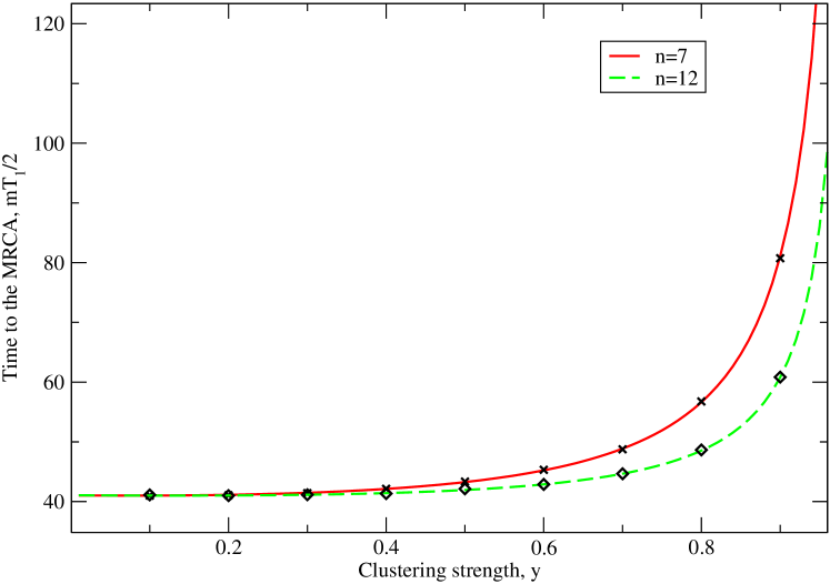
Figure 1: Comparison of numerical calculations of the time to the MRCA $T_{1}$ in the two-level model with $L=84$ demes and two different cluster sizes, $n=7$ and $12$. The curved lines show data from a numerically exact solution, and the points the corresponding averages over $10^{5}$ genealogies generated by Monte Carlo sampling. The sampling error on the latter are smaller than the symbol size.

We now investigate the growth of fixation time with $L$ in the regime where intra-cluster migration is (at least for sufficiently large $L$) faster than inter-cluster migration, and compare the effective number of demes so obtained with the predictions of (53). Of the many possible ways in which the limit $L\to\infty$ can be taken, two are of particular interest to us. In the first, the number of clusters $\ell$ is held fixed whilst the number of demes in each cluster $n$ goes to infinity; the the second, the cluster size $n$ is held fixed as more and more clusters are added.

Since the steady state is uniform, $Q_{i}^{\ast}=\frac{1}{L}$, we find from Eq. (53) that

$$\alpha_{e}=\frac{(n-1)Y_{s}+n(\ell-1)Y_{d}}{1+2yY_{s}+2(1-y)Y_{d}}$$ (56)

where $Y_{s}=Y_{ij}^{(0)}$ for a pair of demes $i,j$ belonging to the same cluster, and $Y_{d}$ the corresponding quantity for two demes from different clusters. The equations (51) become

$$Y_{s} = \frac{1+2n(\ell-1)\nu_{d}Y_{d}}{2[\nu_{s}+n(\ell-1)\nu_{d}]}$$ (57)

$$Y_{d} = \frac{1+2(n-1)\nu_{d}Y_{s}}{2n\nu_{d}}\;.$$ (58)

Substituting the solutions into (56) and taking the limits of interest one finds that

$$\alpha_{e}\sim\left\{\begin{array}[]{ll}\frac{L}{2}&n\to\infty,\;\mbox{fixed $\ell$}\\ \frac{L}{2}\left(1+\frac{y^{2}}{(n-[1-y])(1-y)}\right)&\ell\to\infty,\;\mbox{fixed $n$}\end{array}\right.\;.$$ (59)

That is, in both cases, the relative effective population size $\alpha_{e}$ grows linearly with $L$ asymptotically. This behaviour is seen in the numerical data shown in Fig. 2 (for constant $\ell$) and Fig. 3 (for constant $n$) in which the combination $mT_{1}/2\alpha_{e}$ is plotted, with the predictions for $\alpha_{e}$ given by the above formulæ. Also shown in the figure are fits to the data $mT_{1}/2\alpha_{e}=A+BL^{-\gamma}$, a value of $A\approx 1$ then indicating a correct prediction for $\alpha_{e}$. We see that in for both cases of fixed cluster number ($\ell=12$) and fixed cluster size ($n=12$), the asymptotes for three values of the parameter $y=0.4,0.6$ and $0.8$ are all consistent with a value of $1$, thus demonstrating the accuracy of the predictions of (53) in these instances.

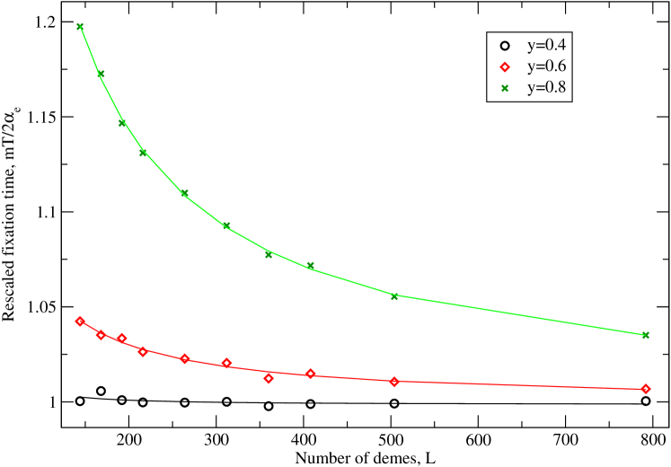
Figure 2: Mean time to the MRCA (and hence to fixation from a single mutant) normalised by the prediction for the effective number of demes for the two-level model as a function of system size with fixed cluster number $\ell=12$ and for $y=0.4,0.6,0.8$. The points show numerical data, with errors of the same order as symbol size. The solid lines are empirical fits $mT/2\alpha_{e}=A+BL^{-\gamma}$. In all cases $A\approx 1$.

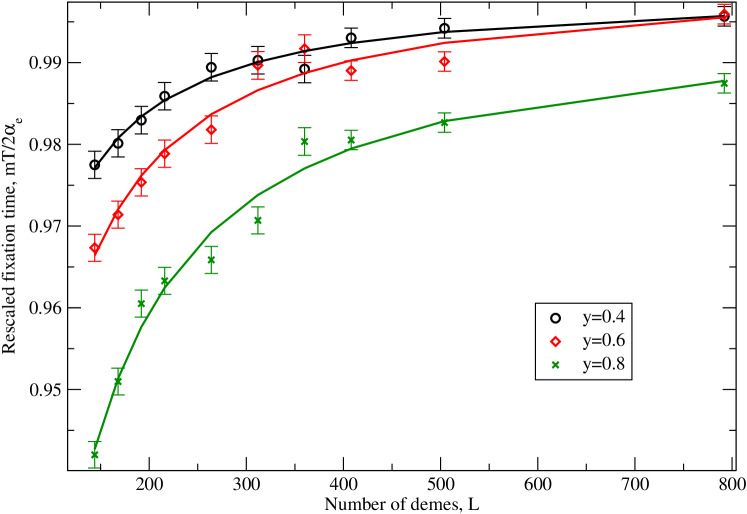
Figure 3: As Fig. 2 but for the case of constant cluster size $n=12$. Again, the solid lines are fits of the form $mT/2\alpha_{e}=A+BL^{-\gamma}$ with asymptotes $A\approx 1$.

5.2.2 Hub-and-spoke model

In the second example model, we also divide the demes into $\ell$ clusters of equal size $n\geq 2$, but this time one of the clusters is a special hub deme with migration between clusters permitted only if one of the two clusters is the hub. The remaining clusters thus form spokes—see Fig. 4. This model is intended to reproduce an effect noticed in social networks, in which some members of a society interact more widely than others; in a biological context, one could perhaps interpret this model as reflecting a continental-archipelago formation, but with a structured population on the continent. Either way, we introduce three independent migration rates: $m_{0}=m\nu_{0}$ for migration between demes within the same cluster; $m_{hs}=m\nu_{hs}$ for migration from a spoke deme to a hub deme (going forwards in time); and the rate $m_{sh}=m\nu_{sh}$ for migration in the opposite direction.

Figure 4: Cartoon of the hub-and-spoke migration model. The demes are divided into $\ell$ clusters, within which migration occurs between every pairs of demes. Migration between demes lying in different clusters is allowed only if one of those demes is in the central hub; spoke-to-spoke migration is prohibited.

There are at least two ways in which one can make a meaningful comparison with the results of the previous section. First, one can impose a uniform overall rate of immigration $m$, with each deme receiving a fraction $y$ of immigrants coming from within the cluster, and the remaining fraction from outside the cluster. In such a case, the parameters appearing in the migration rates are

$$\nu_{0} = \frac{y}{n-1}$$ (60)

$$\nu_{hs}=\nu_{hs}^{(i)} = \frac{1-y}{n(\ell-1)}$$ (61)

$$\nu_{sh}=\nu_{sh}^{(i)} = \frac{1-y}{n}\;.$$ (62)

Alternatively, one can impose a uniform emigration rate, with a fraction $y$ of migrants from each deme remaining within the cluster, and the remainder going elsewhere. This rule is enforced by choosing $\nu_{hs}=\nu_{hs}^{(e)}=\nu_{sh}^{(i)}$ and $\nu_{sh}=\nu_{sh}^{(e)}=\nu_{hs}^{(i)}$. When the symbol $\nu_{hs}$ or $\nu_{sh}$ appears in expressions below, they are valid for either rule once the appropriate expressions in terms of $m$, $y$, $n$ and $\ell$ have been inserted. Note that the diagonal elements of the matrix of migration rates will be altered as a consequence of exchanging the off-diagonal elements so that probability is conserved; note also that for the two-level model, both rules are equivalent.

One property of the hub-and-spoke model is that the stationary state satisfies detailed balance, as one can show by using, e.g., a Kolmogorov criterion (Kelly, 1979). This implies that ratios of stationary probabilities satisfy the relation $Q_{i}^{\ast}/Q_{j}^{\ast}=\nu_{ji}/\nu_{ij}$ where $i$ and $j$ label demes. Introducing $\tilde{Q}_{h}^{\ast}$ for the total probability for the single remaining ancestor of the entire population to reside somewhere in the hub, and its complement $\tilde{Q}_{s}^{\ast}=1-\tilde{Q}_{h}^{\ast}$ for the ancestor to be somewhere in the spoke, we have that $(\ell-1)Q_{h}^{\ast}/Q_{s}^{\ast}=\nu_{sh}/\nu_{hs}$ and so for both rules

$$\tilde{Q}_{h}^{\ast}=\frac{\nu_{sh}}{\nu_{sh}+(\ell-1)\nu_{hs}}\;.$$ (63)

In particular, under uniform immigration one has $\tilde{Q}_{h}^{\ast}=\tilde{Q}_{s}^{\ast}=\frac{1}{2}$. However, since there are (for $\ell>2$) more spoke demes than hub demes, a mutation occurring in the hub is $(\ell-1)$ times more likely to fix than one occurring in the spoke. Under the uniform emigration rule, the opposite is true, a mutation somewhere in the spoke being $(\ell-1)$ times more likely to fix.

A further useful property of the hub-and-spoke model is that the diagonalisation of the matrix $\mathsf{M}$ that is needed to calculate $\tau_{i}-T_{1}$ via Eq. (45) can be done analytically. In fact, only one non-stationary eigenstate contributes. This state has

$$\lambda_{2} = -m\left[n\nu_{sh}+n(\ell-1)\nu_{hs}\right]$$ (64)

$$\mathsf{u}_{2} = (1,-1)$$ (65)

$$\mathsf{v}_{2} = (\tilde{Q}^{\ast}_{s},-\tilde{Q}^{\ast}_{h})^{T}$$ (66)

where the $i^{\rm th}$ element of a column vector notated here as $(h,s)^{T}$ is $h$ if $i$ corresponds to a hub deme, and $s$ otherwise, whilst the corresponding element of row vector $(h,s)$ is $h/n$ for a hub deme, and $s/[n(\ell-1)]$ otherwise. Defined this way, the scalar product $(h,s)\cdot(h^{\prime},s^{\prime})^{T}=hh^{\prime}+ss^{\prime}$, and the stationary solution can be expressed as $\mathsf{u}_{1}=(\tilde{Q}^{\ast}_{h},\tilde{Q}^{\ast}_{s})$ which is orthogonal to $\mathsf{v}_{2}$, as required. With this notation established, it is easy to show that the row vector

$$\mathsf{R}^{\ast}\equiv(\tilde{R}^{\ast}_{h},\tilde{R}^{\ast}_{s})=\mathsf{u}_{1}+\left(\tilde{R}_{h}^{\ast}\tilde{Q}_{s}^{\ast}-\tilde{R}_{s}^{\ast}\tilde{Q}_{h}^{\ast}\right)\mathsf{u}_{2}\;,$$ (67)

where $\tilde{R}_{h}$ and $\tilde{R}_{s}$ are the total probability that the MRCA is somewhere in the hub or a spoke respectively. As a consequence of this relation, we must have $\mathsf{R}^{\ast}\cdot\mathsf{v}_{n}=0$ for $n>2$ by the biorthogonality of the eigenvectors. Therefore, only one term $n=2$ in the sum in (45) contributes, as claimed.

Evaluating (45) for the case of an initial mutation positioned somewhere in the hub, one finds the mean time for subsequent fixation to be

$$\tau_{h} = T_{1}+\frac{1}{Q_{h}^{\ast}}\frac{\mathsf{R}^{\ast}\cdot\mathsf{v}_{2}}{\lambda_{2}}$$ (68)

$$= T_{1}-\frac{1}{|\lambda_{2}|}\left(\frac{R_{h}^{\ast}}{Q_{h}^{\ast}}-1\right)\;.$$ (69)

Written this way, it is evident that when the MRCA is more likely to be in the hub than the single remaining ancestor in the stationary state, the mean time to fixation from the hub is less than that to the MRCA.

Under the uniform immigration rule, the mean time to fixation from the hub is given by

$$\tau_{h}=T_{1}-\frac{2R_{h}^{\ast}-1}{2m(1-y)}\;.$$ (70)

Meanwhile, when uniform emigration is enforced,

$$\tau_{h}=T_{1}-\frac{1}{m(1-u)}\left[(\ell-1)R_{h}^{\ast}-\frac{1}{(\ell-1)^{-1}+(\ell-1)}\right]\;.$$ (71)

The corresponding fixation times from a spoke deme can be found using the fact that $\tilde{Q}_{h}^{\ast}\tau_{h}+\tilde{Q}_{s}^{\ast}\tau_{s}=T_{1}$, as was mentioned at the end of Section 5.1 above.

It remains to find $T_{1}$ and $R_{h}^{\ast}$ numerically; first, however, we obtain a prediction for the effective number of demes using Eq. (53). This is a more involved enterprise than for the two-level model, because there are four distinct ways to sample pairs of individuals from the population: both from the hub cluster (we denote this $hh$), both from the same spoke cluster ($ss$), one from the hub and one from a spoke ($hs$) and two from different spoke clusters ($s\bar{s}$). The set of linear equations (51) then becomes

$$Y_{hh} = \frac{1+2n(\ell-1)\nu_{hs}Y_{hs}}{2\nu_{0}+2n(\ell-1)\nu_{hs}}$$ (72)

$$Y_{ss} = \frac{1+2n\nu_{sh}Y_{hs}}{2\nu_{0}+2n\nu_{sh}}$$ (73)

$$Y_{hs} = \frac{1}{n\nu_{sh}+n(\ell-1)\nu_{hs}}\big{[}1+(n-1)\nu_{hs}Y_{ss}+{}$$ (74)

$$\qquad n(\ell-2)\nu_{hs}Y_{s\bar{s}}+(n-1)\nu_{sh}Y_{hh}\big{]}$$

$$Y_{s\bar{s}} = \frac{1+2n\nu_{sh}Y_{hs}}{2n\nu_{sh}}\;.$$ (75)

These can be readily solved using (for example) a computer algebra package. The formula for relative effective size (53) takes the form

$$\textstyle\alpha_{e}=\frac{(\tilde{Q}_{s}^{\ast})^{2}[(n-1)Y_{ss}+n(\ell-2)Y_{s\bar{s}}]+(\ell-1)\tilde{Q}_{h}^{\ast}[(n-1)\tilde{Q}_{h}^{\ast}Y_{hh}+2n\tilde{Q}_{s}^{\ast}Y_{hs}]}{(\tilde{Q}_{s}^{\ast})^{2}[1+2(n-1)\nu_{0}Y_{ss}+2n\nu_{sh}Y_{hs}]+(\ell-1)(\tilde{Q}_{h}^{\ast})^{2}[1+2(n-1)\nu_{0}Y_{hh}+2n(\ell-1)\nu_{hs}Y_{hs}]}\;.$$ (76)

We shall not present the full expression for $\alpha_{e}$ here, as it is rather complicated and unrevealing. Instead, we shall show only how $\alpha_{e}$ behaves asymptotically for large $L$, under the two immigration rules, and for the two contrasting limits of infinite system size discussed for the two-level model.

In the case where the number of clusters $\ell$ is held fixed, and the number of demes within them $n$ increased, the predicted $\alpha_{e}$ increases linearly with $L$ under both the uniform immigration and emigration rule. Specifically one has for uniform immigration

$$\alpha_{e}\sim\frac{2(\ell-1)}{\ell^{2}}L$$ (77)

and for uniform emigration

$$\alpha_{e}\sim\frac{[1+(\ell-1)^{2}]^{2}}{2\ell^{2}[(\ell-1)+(\ell-2)^{2}y]}L\;.$$ (78)

Simulation data for case of fixed $\ell=12$ are shown in Fig. 5 for uniform immigration and in Fig. 6 for uniform emigration. In both figures the combination $mT/2\alpha_{e}$ is plotted for three different values of $y$ ($y=0.4,0.6,0.8$). In all cases fits to the data of the form $A+BL^{-\gamma}$ reveal an asymptote $A$ consistent with unity; that is, the data show an asymptotic linear growth with the slope predicted by the effective size formula (53). In both cases, the relative variation of fixation time with the location of the first mutation vanishes in the limit $L\to\infty$. That this should be the case can be seen from the formulæ in Eq. (70) and (71); when $\ell$ is fixed, the correction term is bounded whilst $T_{1}$ grows linearly $L$.

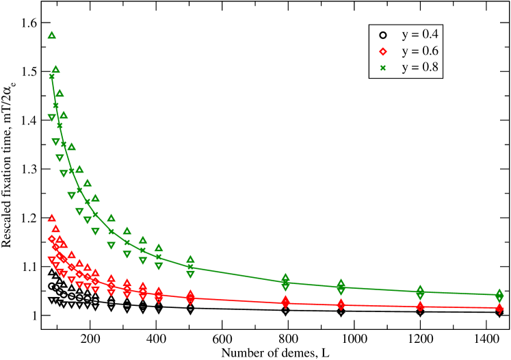
Figure 5: Mean time to fixation and the MRCA, normalised by the relative effective population size $\alpha_{e}$, in the hub-and-spoke model under the uniform immigration rule for $y=0.4,0.6,0.8$ and increasing deme number $L$ with fixed cluster number $\ell=12$. The upward- and downward-pointing triangles show fixation times from the spoke $\tau_{s}$ and hub $\tau_{h}$ respectively, whilst the points in between are the MRCA times. The solid lines show fits to the latter of the form $mT_{1}/2\alpha_{e}=A+BL^{-\gamma}$; in all three cases the asymptote $A\approx 1$.

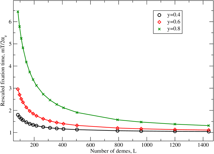
Figure 6: As Fig. 5, but for the uniform emigration rule. In this case, the mean fixation times from both hub and spoke are indistinguishable from the mean time to the MRCA, so only the latter has been plotted. The solid lines show fits of the form $mT_{1}/2\alpha_{e}=A+BL^{-\gamma}$, and show asymptotes $A\approx 1$ in all cases.

A scaling of the fixation time that is nonlinear in $L$ is seen when the number of demes is increased by adding more and more spokes of fixed size $n$. In this limit, the prediction for $\alpha_{e}$ asymptotes to a constant

$$\alpha_{e}\sim 2\frac{(n-1)^{2}}{n-(1-y)}+\frac{5}{4}\frac{1}{1-y}$$ (79)

under the uniform immigration rule, but increases quadratically with $L$ as

$$\alpha_{e}\sim\frac{1}{2n^{2}(1-y)}L^{2}$$ (80)

as $L\to\infty$. Plotting the quantity $mT_{1}/2\alpha_{e}$ for the case $n=12$ suggests that this asymptotic quadratic growth is correctly predicted, shown by the approach to a constant value as $L\to\infty$ in Fig. 7. Again fits to the data suggest asymptotes consistent with unity, showing the accuracy of the prediction given by the effective relative population size (53). In Fig. 8, data for the uniform immigration rule with constant cluster size $n=12$ are shown for the case $y=0.8$ (data for other $y$ values show similar behaviour, but have been omitted for clarity). Even at the system sizes shown, the fixation time is still growing with $L$. However, the data are suggestive that eventually the fixation time will saturate to a constant as predicted by Eq. (53). First, a fit to the data of the form $A+BL^{-\gamma}$ suggests an asymptote of $A\approx 1.38$, that is, that the fixation time is bounded by a constant but one that is approximately $40\%$ larger than that predicted by (53). (The asymptote for smaller values of $y$ is also underestimated by (53), but not to such a great extent: the numerical data exceed the prediction by about $10\%$ for $y=0.4$ and about $20\%$ for $y=0.6$). Further evidence for the fixation time remaining bounded in the limit $L\to\infty$ is provided by the fact that—uniquely among the models and limits considered—the relative differences between the mean times to fixation and the MRCA remain finite in the limit $L\to\infty$. As noted above, the absolute differences are bounded and so relative differences may remain finite only if the fixation time saturates.

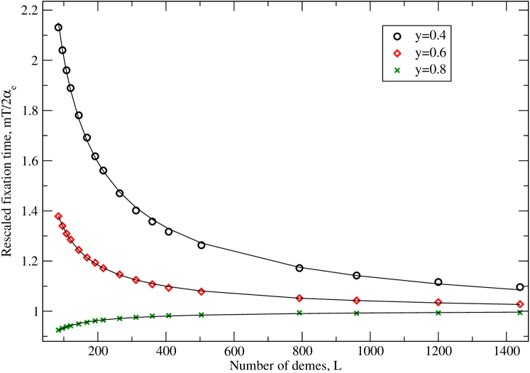
Figure 7: As Fig. 5 but for the uniform emigration rule and increasing $L$ as the cluster size is held fixed at $n=12$. Here the points show numerical estimates of the mean time to the MRCA for $y=0.4,0.6,0.8$; again the mean fixation times from hub and spoke are indistinguishable from these data. The solid lines are fits of the form $mT/2\alpha_{e}=A+BL^{-\gamma}$, with $A\approx 1$ in all three cases.

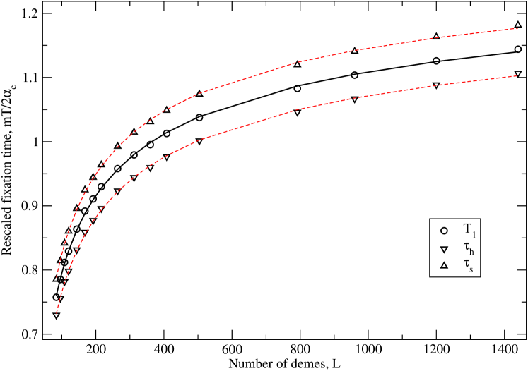
Figure 8: As Fig. 5, but for the uniform immigration rule and increasing $L$ as the cluster size is held fixed at $n=12$. Here, the points show numerical data for the case $y=0.8$; those for other $y$ values are similar and have been omitted for clarity. The solid lines are fits of the form $mT/2\alpha_{e}=A+BL^{-\gamma}$.

6 Discussion and conclusion

The aim of this work was to develop a better understanding of the effects of population subdivision on fixation under neutral genetic drift. This was achieved by exploiting a connection between forward- and backward-time properties of neutral genetic drift which admitted the derivation of a number of new results for fixation properties in subdivided populations that are exact in the limit of extemely slow migration. Since the underlying motivation was partly to assess the viability of genetic drift as a mechanism for propagating a social change, we were particularly interested in establishing how fixation times grow with the number of demes. Furthermore, the existence of historical data requires knowledge of variation of fixation times with the initial distribution of mutants.

We address the matter of variation first. It is clear from the elementary considerations leading to Eq. (7) that fixation probability can vary greatly with the initial location of mutants. For example, if one has in the hub-and-spoke model a mutation which is known to be located in the hub, it is $(\ell-1)$ times more likely to invade the whole population than the same mutation occurring in a spoke, as long as the uniform immigration rule is applied. Thus, if the number of spokes is very large, one can approach near certainty for a mutation to fix by genetic drift alone. However, this is balanced by the fact that there are $(\ell-1)$ fewer hub demes than spoke demes, so a mutation occurring at a random location is as unlikely to fix in this subdivided population as any other with the same overall size. We contrast again with the findings of Lieberman et al. (2005) which showed almost certain fixation from a random initial condition driven by selection in a spatially structured population. Such behaviour can also arise without the need for selection as long as one is able to position the initial mutations strategically, as would be the case when one is constrained by historical data.

Conversely, we observed only minor variation with the initial condition in the mean fixation time, averaged over those realisations of the dynamics where fixation actually occurs. This was seen both in new exact results for Wright’s island model (Section 4) and in numerical data for clustered models (Section 5.2). In fact, in all cases the relative magnitude of variation vanishes in the limit of an infinite system, except possibly in the case where the fixation time remained constant in that limit. However, even there, the variation was of the order of a few percent. This lack of variation has two practical benefits. First, one may as well approximate any historical data by a random initial condition with the same overall frequency of mutants, and use Eq. (22) to calculate fixation times from the coalescence times $T_{n}$ which are easy to obtain numerically. We remark that this formula can easily be generalised to find higher cumulants of the fixation time distribution. The second benefit is that if one notices considerable variation of fixation times in historical data, it may then be possible to rule out genetic drift as a propagation mechanism as a consequence. Finally, on the subject of variation, a curiosity that emerged from the exact analysis of Wright’s island model was evidence for mean time to fixation to be minimised (subject to a constraint of a fixed overall mutant frequency) by a random initial condition. It would be interesting to show this more rigorously, and to see if this is also the case for a wider class of models.

By considering the fate of a single mutation in models that had demes grouped into tightly-knit clusters, we established three different growth laws for the fixation time under various conditions: linear (as in Wright’s island model), quadratic and approach to a constant. The latter scenario is, of course, the most intriguing, since then one has a population-level change occurring in an infinite population in a finite time through genetic drift alone. The origin of this phenomenon lies in the nonconservative nature of the migration process in place: the total number of individuals entering the spokes from the hub under the constant immigration rule vastly exceeds the number entering the hub. This has the consequence that, as one goes backward in time, the probability of finding pair of lineages in a vanishingly small region of space (the hub) remains finite as the number of demes is increased; thus their coalescence, and hence fixation, can occur in a finite time. By contrast, under the uniform emigration rule, the probability that lineages are found in separate spokes is finite, and one must wait a long time until they are both present in the same deme: this drives the superlinear increase in fixation time. Although in a biological context the hub-and-spoke model may be of limited application, one can think of this enhancement of offspring number as a form of spatially-dependent selection and it would perhaps be of interest to see if a similar effect is evident in potentially more realistic situations where the deme sizes are small and their number restricted by topological considerations.

On the other hand, in the cultural context of language change where migration corresponds to a speaker retaining a record of another’s utterances, there is no particular reason to assume conservative migration. In fact, a uniform immigration rule as implemented in this work arises rather naturally, as it corresponds to every speaker dividing the same amount of attention equally between each person she listens to. Furthermore, the hub-and-spoke model probably better reflects the nature of social interactions, in which some members of society have more long-range connections than others. It is unclear, however, if the phenomenon of a finite fixation time will be seen for infinite populations on more realistic social networks. We are currently investigating this possibility, and results will be reported in due course.

Finally, we compared results from simulations with predictions from a formula for effective population size, Eq. (5) whose general form was given by Rousset (2004) and that was specialised here to the extreme slow migration limit in which all migration rates are inversely proportional to the deme size and have a vanishingly small coefficient. The resulting formula, (53), was found to give precise predictions for the fixation time in the limit of an infinite number of demes for all models considered, except when the fixation time appears to be bounded by a constant; here, the predicted asymptote was seen to be exceeded by as much as $40\%$. This would suggest that in this particular case, the fixation time is not well characterised by the asymptotic coalescence rate that appears on the right-hand side of Eq. (5). To explore this possibility, it is worth considering the extreme case of two demes with arbitrary migration rates $m_{12}=m\nu_{12}$, $m_{21}=m\nu_{21}$ in the extreme slow migration limit $m\to 0$. If one starts with one lineage per deme in this model, the rate of coalescence between these lineages is $c=m_{12}+m_{21}$, since that is the rate at which one of the lineages hops from one deme to another, at which time a coalescence immediately takes place (as least in the limit $m\to 0$). By contrast, the mean asymptotic rate of coalesence given by the asmyptotic effective size formula (53) is $c/[2Q_{1}^{\ast}(1-Q_{1}^{\ast})]$ where $Q_{1}^{\ast}=m_{21}/(m_{12}+m_{21})$. For any choice of migration rates, the true rate of coalescence between the last pair of lineages is overestimated by a least a factor of $2$, and hence the effective population size underestimated as was seen for the hub-and-spoke model. This two-demes model provides an extreme example of a case where all coalesences occur before the onset of the asymptotic regime. We believe this is also what is happening in the hub-and-spoke model, and could further explain why this is the only case in this work in which any variation of fixation time with initial condition was observed. Through more careful considerations of the relevant coalescence events (Rousset, 2004), one anticipates that better predictions for the fixation time can be obtained.

We end by remarking that if one is only interested in the general scaling of the fixation time with the number of demes (and not in precise estimates of the coefficients), the simple formula of Nagylaki (1980), $N_{e}^{-1}=\sum_{i}(Q_{i}^{\ast})^{2}/N_{i}$, is much easier to apply than the full expression (5) and can be used as long as lineages are well mixed by the dynamics and fluctuation effects are unimportant. An example of a model in which this simple formula gives the wrong prediction for scaling is the stepping-stone model in two dimensions and less (Slatkin, 1991; Rousset, 1997; Cox and Durrett, 2002). It is also perhaps worth noting that the stepping-stone model in the slow-migration limit $m\to 0$ is equivalent to the particle reaction system $A+A\to A$ that has been of interest to physicists (Peliti, 1986; ben Avraham, 1998). The methods that have been employed in this context allow, in principle, the distribution of ancestors $Q(C|D;t)$ appearing in the general relation (10) to be calculated for the stepping stone model in one dimension. It would be interesting to exploit this connection to obtain further new results for the properties of fixation in subdivided populations.

References

- Barton (1993) Barton, N. H., 1993. The probability of fixation of a favoured allele in a subdivided population. Genet. Res. Camb. 62, 149–157.
- Baxter et al. (2006) Baxter, G. J., Blythe, R. A., Croft, W., McKane, A. J., 2006. Utterance selection model of language change. Phys. Rev. E 73, 046118.
- ben Avraham (1998) ben Avraham, D., 1998. Complete exact solution of diffusion-limited coalescence, . Phys. Rev. Lett. 81, 4756–4759.
- Charlesworth et al. (2003) Charlesworth, B., Charlesworth, D., Barton, N. H., 2003. The effects of genetic and geographic structure on neutral variation. Annu. Rev. Ecol. Evol. Syst. 34, 99–125.
- Cherry and Wakeley (2003) Cherry, J. L., Wakeley, J., 2003. A diffusion approximation for selection and drift in a subdivided population. Genetics 163, 421–248.
- Christiansen and Kirby (2003) Christiansen, M. H., Kirby, S. (Eds.), 2003. Language Evolution. Oxford University Press, Oxford.
- Cox and Durrett (2002) Cox, J. T., Durrett, R., 2002. The stepping stone model: new formulas expose old myths. Ann. Appl. Prob. 12, 1348–1377.
- Crow and Kimura (1970) Crow, J. F., Kimura, M., 1970. An Introduction to Population Genetics. Harper and Row, New York.
- Donnelly and Tavaré (1995) Donnelly, P., Tavaré, S., 1995. Coalescents and genealogical structure under neutrality. Annu. Rev. Genet. 29, 401–421.
- Fisher (1930) Fisher, R. A., 1930. The Genetical Theory of Natural Selection. Clarendon Press, Oxford.
- Gordon et al. (2004) Gordon, E., Campbell, L., Hey, J., MacLagan, M., Sudbury, A., Trudgill, P., 2004. New Zealand English: its Origins and Evolution. Cambridge University Press, Cambridge.
- Gradshteyn and Ryzhik (2000) Gradshteyn, I. S., Ryzhik, I. M., 2000. Table of Integrals, Series and Products. Academic Press, San Diego.
- Griffiths (1984) Griffiths, R. C., 1984. Asymptotic line-of-descent distributions. J. Math. Biology 21, 67–75.
- Grimmett and Stirzaker (2001) Grimmett, G., Stirzaker, D., 2001. Probability and Random Processes. Oxford University Press, Oxford.
- Kelly (1979) Kelly, F. P., 1979. Reversibility and stochastic networks. Wiley, Chichester.
- Kimura and Ohta (1969) Kimura, M., Ohta, T., 1969. The average number of generations until fixation of a mutant gene in a finite population. Genetics 61, 763–771.
- Kingman (1982) Kingman, J. F. C., 1982. The genealogy of large populations. Journal of Applied Probability 19: Essays., 27–43.
- Latter (1973) Latter, B. D. H., 1973. The island model of population differentiation: a general solution. Genetics 73, 147–157.
- Lieberman et al. (2005) Lieberman, E., Hauert, C., Nowak, M. A., 2005. Evolutionary dynamics on graphs. Nature 433, 312–316.
- Maruyama (1970a) Maruyama, T., 1970a. Effective number of alleles in a subdivided population. Theor. Popul. Biol. 1, 273–306.
- Maruyama (1970b) Maruyama, T., 1970b. On the fixation probability of mutant genes in a subdivided population. Genet. Res. Camb. 15, 221–225.
- Möhle (2001) Möhle, M., 2001. Forward and backward diffusion approximations for haploid exchangeable population models. Stoch. Process. Appl. 95, 133–149.
- Moran (1958) Moran, P. A. P., 1958. Random processes in genetics. Proc. Cambridge Phil. Soc. 54, 60–71.
- Nagylaki (1980) Nagylaki, T., 1980. The strong migration limit in geographically structured populations. J. Math. Biology 9, 101–114.
- Nei and Takahata (1993) Nei, M., Takahata, N., 1993. Effective population size, genetic diversity, and coalescence time in subdivided populations. J. Mol. Evol. 37, 240–244.
- Nordborg and Krone (2002) Nordborg, M., Krone, S. M., 2002. Separation of time scales and convergence to the coalescent in structured populations. In: Slatkin, M., Veuille, M. (Eds.), Modern Developments in Theoretical Population Genetics: The Legacy of Gustave Malécot. Oxford University Press, pp. 194–232.
- Notohara (1990) Notohara, M., 1990. The coalescent and the genealogical process in geographically structured population. J. Math. Biology 29, 59–75.
- Notohara (2001) Notohara, M., 2001. The structured coalescent process with weak migration. J. Appl. Prob. 38, 1–17.
- Peliti (1986) Peliti, L., 1986. Renormalisation of fluctuation effects in the reaction. J. Phys. A 19, L365–L367.
- Rousset (1997) Rousset, F., 1997. Genetic differentiation and estimation of gene flow from F-statistics under isolation by distance. Genetics 145, 1219–1228.
- Rousset (2003) Rousset, F., 2003. Effective size in simple metapopulation models. Heredity 91, 107–111.
- Rousset (2004) Rousset, F., 2004. Genetic structure and selection in subdivided populations. Princeton University Press, Oxford.
- Roze and Rousset (2003) Roze, D., Rousset, R., 2003. Selection and drift in subdivived populations: a straightforward method for deriving diffusion approximations and applications involving dominance, selfing and local extinctions. Genetics 165, 2153–2166.
- Sjödin et al. (2005) Sjödin, P., Kaj, I., Krone, S., Lascoux, M., Nordborg, M., 2005. On the meaning and existence of an effective population size. Genetics 169, 1061–1070.
- Slatkin (1981) Slatkin, M., 1981. Fixation probabilities and fixation times in a subdivided population. Evolution 35, 477–488.
- Slatkin (1991) Slatkin, M., 1991. Inbreeding coefficients and coalescence times. Genet. Res. Camb. 58, 167–175.
- Slatkin and Voelm (1991) Slatkin, M., Voelm, L., 1991. Fst in a hierarchical island model. Genetics 127, 627–629.
- Takahata (1991) Takahata, N., 1991. Genealogy of neutral genes and spreading of selected mutations in geographically structured populations. Genetics 129, 585–595.
- Trudgill (2004) Trudgill, P., 2004. New-dialect formation: the inevitability of colonial Englishes. Edinburgh University Press, Edinburgh.
- Wakeley (1998) Wakeley, J., 1998. Segregating sites in wright’s island model. Theoret. Popul. Biol. 53, 166.
- Wakeley (2001) Wakeley, J., 2001. The coalescent in an island model of population subdivision with variation among demes. Theoret. Popul. Biol. 59, 133–144.
- Wakeley (2004) Wakeley, J., 2004. Recent trends in population genetics: more data! more math! simple models? J. Hered. 95, 397–405.
- Wakeley (2005) Wakeley, J., 2005. The limits of theoretical population genetics. Genetics 169, 1–7.
- Wakeley and Aliacar (2001) Wakeley, J., Aliacar, N., 2001. Gene genealogies in a metapopulation. Genetics 159, 893–905.
- Wakeley and Lessard (2006) Wakeley, J., Lessard, S., 2006. Corridors for migration between large subdivided populations, and the structured coalescent. In press.
- Wakeley and Takahashi (2004) Wakeley, J., Takahashi, T., 2004. The many-demes limit for selection and drift in a subdivided population. Theor. Popul. Biol. 66, 83–91.
- Whitlock (2002) Whitlock, M. C., 2002. Fixation probability and time in subdivided populations. Genetics 164, 767–779.
- Whitlock and Barton (1997) Whitlock, M. C., Barton, N. H., 1997. The effective size of a subdivided population. Genetics 146, 427–441.
- Wilkinson-Herbots (1998) Wilkinson-Herbots, H. M., 1998. Genealogy and subpopulation differentiation under various models of population structure. J. Math. Biology 37, 535–585.
- Wright (1931) Wright, S., 1931. Evolution in mendelian populations. Genetics 16, 97–159.