Why are diploid genomes widespread and dominant mutations rare?

Diana Garncarz¹, Stanislaw Cebrat¹, Dietrich Stauffer^1,2 and Klaus Blindert²

¹Department of Genomics, Institute of Genetics and Microbiology, University of Wrocław,

ul. Przybyszewskiego 63/77, PL-54148 Wrocław, Poland

² Institute for Theoretical Physics, Cologne University, D-50923 Köln, Euroland.

Abstract

We have used the sexual Penna ageing model to show that the relation between dominance and recessiveness could be a force which optimizes the genome size. While the possibility of complementation of the damaged allele by its functional counterparts (recessiveness) leads to the redundancy of genetic information, the dominant effect of defective genes tends to diminish the number of alleles fulfilling the same function. Playing with the fraction of dominant loci in the genome it is possible to obtain the condition where the diploid state of the genome is optimal. If the status of each bit position as dominant or recessive mutations is changed for each individual randomly and rarely, then after a long time a stationary equilibrium of many recessive and few dominant loci is established in the sexual Penna model. This effect vanishes if the same changing distribution of dominant loci applies to all individuals.

1 Introduction

Recent advances in the genome analyses have indicated that genomes of the closely related species can differ substantially in their sizes. To stress the flexibility of the genome structure and size, the phenomenon is called sometimes ”the DNA (genome) in flux”. There are many mechanisms, at different levels of genome organization, which influence the genome size. Some very sophisticated mechanisms rearrange specific sites inside the genome during the development. These mechanisms eliminate some sequences from the genome but the changes are not inherited because the programmed excisions take place in the somatic cells being out of the germ line, like rearrangements of genes coding for immunoglobulins or T cell receptors in lymphocytes [1]. Some DNA excisions lead to generation of the new functions of the cell but simultaneously stop the cell divisions like in the case of generation of the nitrogenase gene in blue algae [2]. Some changes could be very minute, adding or eliminating single nucleotides, or they could be very substantial, adding or eliminating genes, clusters of genes, whole haplotypes or even duplicating whole genomes. Additions or deletions of small numbers of nucleotides, if inside coding sequences, usually are deleterious for the functions of the sequences (genes) and the negative selection eliminates the mutants. Addition of a complete coding sequence, called gene duplication, produces redundant information in the genome (paralog genes). The additional copy of the gene can stay in the genome if it complements the function of its homolog, enhances this function or by any other means helps the host to compete with other organisms. If the copy is dispensable, it is lost during later evolution due to neutral selection.

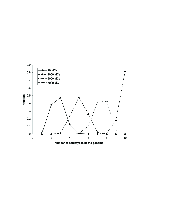
Figure 1: Diagrams showing the increasing numbers of haplotypes in the genomes during the simulations when all defective genes were recessive.

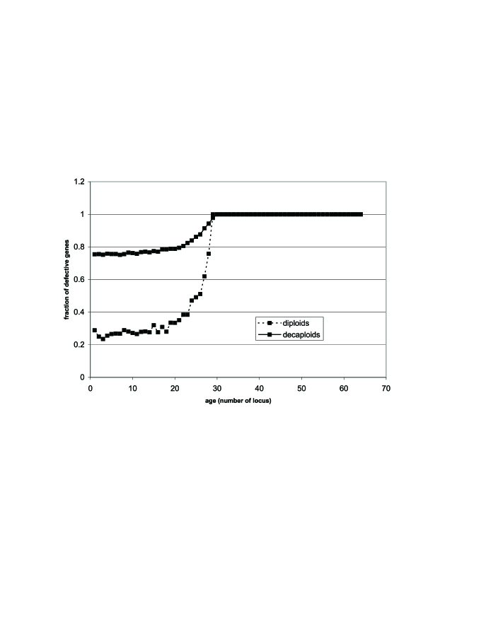
Figure 2: Distribution of defective genes in the genetic pool of the population depending on time of their expression for diploid and decaploid genomes (two or ten haplotypes in the genome, respectively).

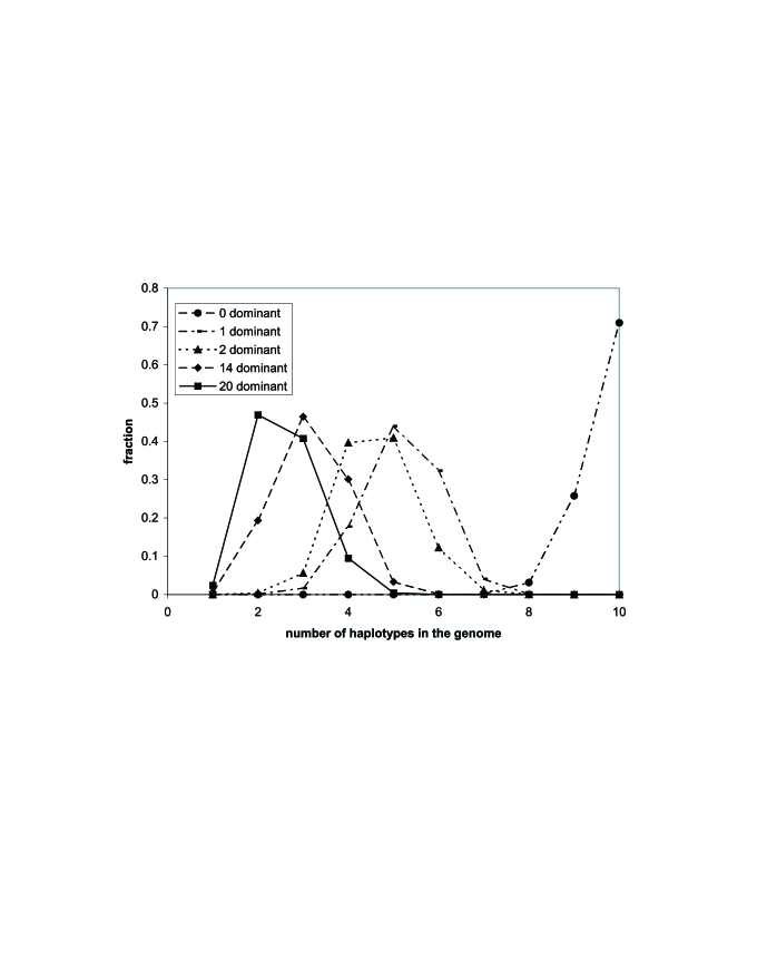
Figure 3: Diagrams showing the numbers of haplotypes in the individual genomes with different number of declared dominant loci (dominant loci were situated as the first ones in the genomes).

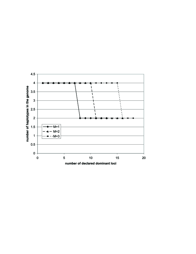
Figure 4: Transition from tetraploid state to diploid state when the number of declared dominant loci increased for different mutational pressure.

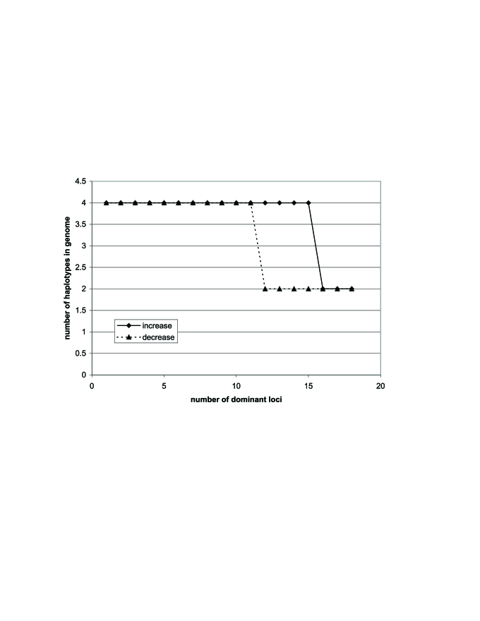
Figure 5: Stabilization of diploid state. After increase in the number of dominant loci to 16 all genomes became diploid, but they stayed diploid when the number of dominant loci was decreased in these genomes to 12. Mutation rate in these simulations: $M=1$.

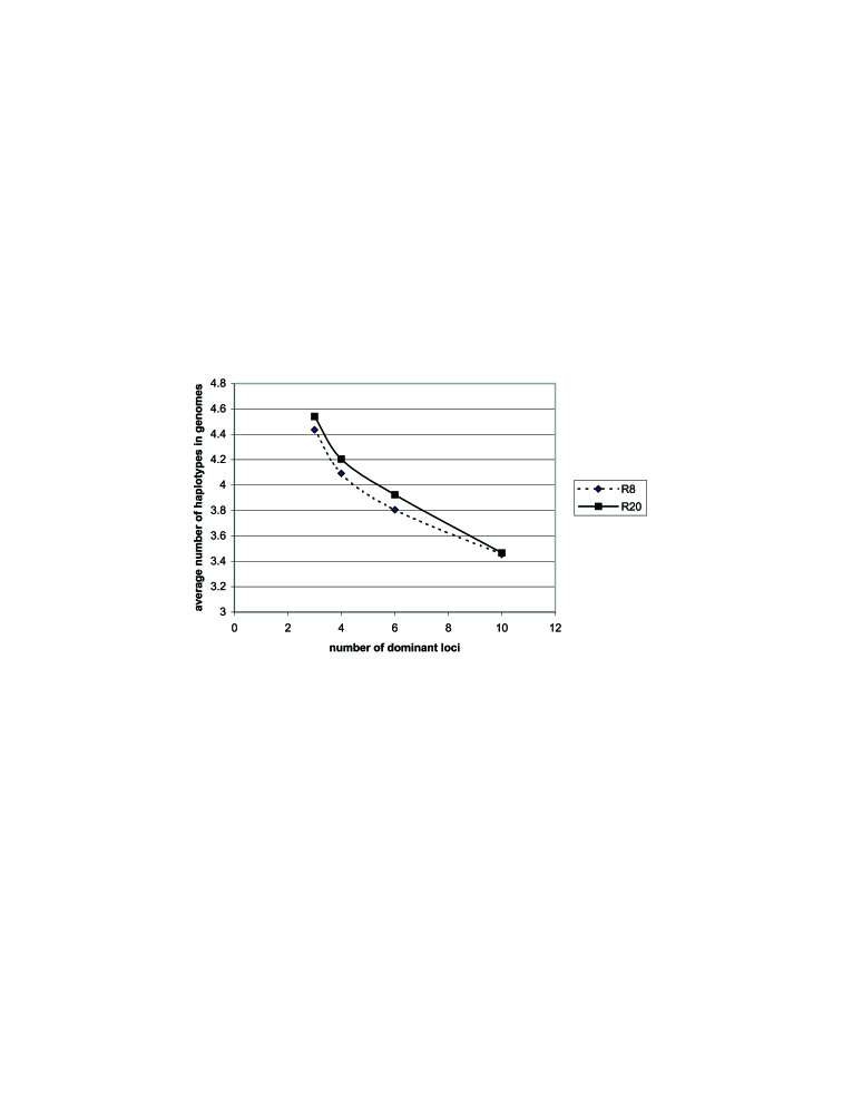
Figure 6: Relation between the number of dominant loci and the average ploidy of genomes for different minimum reproduction ages.

In this paper we are going to discuss and to model only some major events which duplicate the whole genomic information. A single, complete set of genomic information is called a haplotype. Organisms or cells possessing one such set are called haploids. If an organism possesses two homologous haplotypes, it is called diploid, if more, polyploid. In some instances whole genomes can be duplicated. Such a duplication of a haploid genome is called diploidization. In fact some normal, developmental processes like sexual reproduction of yeasts could be considered as diploidization. Two haploid cells with homologous haplotypes fuse together and form one diploid cell. In this case the process could be considered reversible - diploid cells even after many generations can again produce haploid cells. If we neglect the existence of homologous genes which could fulfill the same function in one haplotype (i.e. duplicated genes, paralogs) we can assume that each function of the haploid organism is performed by a single copy of a gene. If the gene is destroyed, its function is also destroyed and if it is important for survival, the whole organism is eliminated. In diploid organisms each gene exists in two copies. Destroying one copy of the gene does not necessarily lead to depriving the organism of the function. The other copy of the gene can ”complement” the function of the homologous destroyed gene. This phenomenon is called recessiveness. Thus, it seems obvious that diploid organisms should be much more robust and resistant to the mutational pressure than haploids because both homologous genes (localized at the corresponding positions in the haploid genomes: loci) have to be destroyed to eliminate the function. The recessiveness is not the only advantage which can be provided by the diploidization. The homologous genes in one locus (alleles) could be slightly different and could provide slightly different genetic information which could be also advantageous for the organism, as in the case of many loci involved in the immunological processes. If we assume that diploidization is such an ingenious invention of the Nature, why is the higher polyploidization not exploited more often? In fact some higher polyploidizations have been observed many times, especially in plant genome evolution [5], [6]. The polyploidization events usually are followed by the genome reduction which leads back to the diploidization [7] and the only effect of the ancient polyploidization is the relatively high number of paralogs, some of them can lose their functions (nonfunctionalization) [3] or some of them can preserve their function for long time [4].

Computer modeling of polyploidization has shown that multiplying the whole set of haplotypes could be profitable for organisms [8]. If the recessiveness of all mutations was assumed and the polyploidy was introduced as an evolving feature of the genomes, the number of haplotypes in organisms had a tendency to grow to the infinity. Nevertheless, parallel to the polyploidization, the genetic load (the fraction of defective alleles) in these genomes also grew. One can conclude that such a polyploidization leads to the accumulation of a high fraction of redundant information which is allowed to be destroyed by mutations. Unfortunately, in Nature, keeping even destroyed information is costly. High energetic costs are paid for the DNA replication and often for the expression of wrong or dispensable information. When the costs of genome replication were introduced into the model by elongating the generation time of the organism proportionally to its genome, the tendency to polyploidization was reduced [8]. On the other hand, declaring all loci recessive is an oversimplification. In fact, not all mutations are recessive and sometimes the function of a single defective copy of a gene cannot be complemented by its wild allele. There are known mutations in the single copy of a gene which lead to deleterious, even lethal effects (such mutations are called dominant). Among the numerous examples of dominant mutations is a dynamic mutation in the gene responsible for Huntington chorea or mutations in the cellular protooncogenes. Mutations in the later group of genes, even in somatic cells, could induce cancer followed by death of the whole multicellular organism. Thus, it seems that polyploidization could be restricted also by the effect of dominance. Since the probability of mutation in a single locus linearly depends on the number of alleles in the locus, the deleterious effects of dominant mutations should be enhanced in the polyploid genomes. Sousa et al. [9] have shown such an effect in the computer simulations when analyzing different strategies of sexual reproduction. They introduced the dominant loci into the simulated genomes and showed that a triploid phase is not an efficient strategy in reproduction.

To simulate the effect of dominance in the phenomenon of the genome polyploidization we have used a modification of the sexual Penna ageing model [10] which enables the study of the influence of different genetic parameters on the population size, age distribution or structure of its genetic pool.

2 Model

In our version of the Penna model each individual is represented by its genome which could consist of different number of haplotypes. One haplotype is a bitstring $64$ bits long. The value of each bit could be $0$, which represents the wild type (correct) gene or $1$, which represents a defective gene. The bits in the strings are numbered consecutively and bits placed at the same position (locus) in different strings represent alleles. If a given locus is declared a dominant one - even one bit set for $1$ at this position determines the defective phenotype of the locus. If a locus is declared a recessive one, it means that all bits at this position have to be set for $1$ to determine the defective phenotype. Otherwise, the phenotype of this locus is correct. Like in the standard Penna model, genes in the loci are switched on chronologically, in the first step all alleles at the first locus are switched on, in the second step the alleles of the second locus are switched on and so on. If the declared number $T$ of defective phenotypes has been expressed, the organism dies. If before dying, the organism reaches the minimum reproduction age, it produces two gametes (see below). One of these two gametes randomly drawn is joined with a gamete produced by another individual of reproductive age and forms a ”newborn” which will be one step old in the next step if it survives the ”Verhulst test”. To avoid the overcrowding of the environment, the logistic equation of Verhulst is introduced to control the birthrate; $V=1-N_{t}/N_{\max}$, where $V$ describes the survival probability of the newborn, $N_{t}$ corresponds to the actual size of the population and $N_{\max}$ is called the maximum capacity of the environment. If a newborn passes the Verhulst test it could die in the future because of too many defective phenotypes switched on or because of reaching the maximum age which equals the number of bits in the string.

Simulations start with a fraction of haploids - 0.25, diploids - 0.25 and triploids - 0.5, all bits are set for $0$, the threshold $T$ is declared $3$, the minimum reproduction age is set for $8$ and birth rate is $1$. In this version of the model the most critical is the production of gametes and newborns. Before this procedure, a declared number of mutations $M$ is introduced into randomly chosen loci of each haplotype of the reproducing parent. If the chosen bit is $0$ it is replaced by $1$ if it is already $1$ it stays $1$ which means that there are no reversions. Next, haplotypes are randomly paired and one recombination (crossover) takes place at a random point in each pair. If the number of haplotypes in the individual genome is not even, one haplotype does not recombine. After recombination haplotypes from each pair are assorted randomly into two gametes. Note that if the number of haplotypes in the parental genome was not even, one gamete would have more haplotypes than the other one. After forming the individual by the fusion of two gametes, its genome could shrink or grow with equal probability by random choice of one haplotype and its elimination or replication.

3 Results and Discussion

The first simulations with all loci declared recessive have shown that the number of haplotypes in the genomes has a tendency to grow to infinity supporting the results previously obtained by Alle [8]. To save computer time we have set the upper limit of polyploidy at 10 (Fig. 1). There are two versions of introducing the limit: in the first one, when the polyploidy of a newborn after gamete fusion reaches 10 it can loose one haplotype with the probability 0.5 but it cannot gain another one. In the second version polyploidy stays at 10. After introducing the first rule, most of individuals reach ”decaploidy” but there is always a fraction of individuals with less than 10 haplotypes. In the second version, all individuals in the populations reach decaploidy. This is not the only difference between the versions. In the standard Penna model simulations, at equilibrium, the genetic pool of the population is characterized by a specific gradient of fractions of defective genes. The fractions stay constant and low for all loci expressed before the minimum reproduction age, grow in the loci expressed after the minimum reproduction age and reach $1$ for the last loci in the bitstrings. This characteristic structure of the genetic pool is observed in the populations when the individuals reaching the upper limit of haplotypes stay with this number and when in equilibrium all genomes are decaploid (Fig. 2). If the number of haplotypes in the decaploid newborn genomes may be reduced, the population does not reach the characteristic distribution of defective genes.

The tendency to the unlimited growth of polyploidy can be reduced by declaring the dominant loci. In the simulations, different numbers of loci were declared dominant (always at the beginning of the bitstrings). The diagrams showing the distributions of the number of haplotypes in the genomes for populations with different numbers of declared dominant loci are shown in Fig. 3. The increase in the number of dominant loci is associated with the decrease in the average number of haplotypes in the genomes. Since introducing the dominant loci into the genomes reduced the tendency to polyploidization, in further simulations we have set the upper limit of polyploidization for $4$. Now, during reproduction, only two types of gametes could be produced: haploid and diploid. The zygotes could be diploid, triploid or tetraploid but one haplotype of triploid zygotes was replicated or lost with equal probability - 0.5. Thus, in the populations the genomes could be either diploid or tetraploid. When we increased the declared number of dominant loci we observed transition from tetraploidy to diploidy (Fig.4). To reach the pure diploid population in the equilibrium, a substantial fraction of active loci in the genomes have to be declared dominant. But when the population already reaches the state of diploidy, it is stable even when the fraction of dominant loci diminishes. It is also possible to get the diploid population with a lower fraction of declared dominant loci when the mutational pressure is increased (Fig. 5). In the Penna model, the number of active loci in the genome (maximum life expectancy) grows with increasing minimum reproduction age. We have checked if the effect of dominance on the evolution of polyploidy depends on the number of dominant loci or the fraction of dominant loci. To estimate that, we have compared the average polyploidy in populations with minimum reproduction age 8 and 20 and the same number of declared dominant loci. The results suggest that the effect depends on the number of dominant loci rather than on the fraction of dominant loci (Fig. 6).

Figure 7: Self-organisation of average number $<d>$ of dominant loci, among a total of 32 loci, at $p=0.01$.

Figure 8: Distribution of the number $d$ of dominant loci in same simulation as in Fig.7.

Figure 9: Distribution (x) of the number $d$ of dominant loci in same simulation as in Fig.7. The straight line at 455 million indicates the case of half the loci being dominant for this statistics. The plus signs show the number of mutated bits: All bits at old age are mutated.

Figure 10: Distribution (x) of the number $d$ of dominant loci with Verhulst applied to newborns only, $B=1$, and only one distribution of dominant loci for the whole population. The plus signs show the distribution of the number $d$ of dominant loci in this simulation. The horizontal line correponds to half the loci dominant and the other half recessive.

4 Emergence of Dominance

In the above sections we have shown that an increasing fraction of dominant loci forces the organisms to restrict the number of haplotypes in the single genome. Now, the question is: what would be the fraction of dominant loci if it could freely evolve in the population with diploid genomes.

Usually, the characterisation of a locus (bit position) as dominant or recessive is fixed initially as the same for all individuals: a dominance bit-string has 6 randomly selected bits set to one and the other 26 set to zero if bit-strings of length 32 are used. These numbers correspond to the empirical fact that recessive diseases are much more widespread than dominant ones.

We now undertake a more realistic simulation by letting this distribution of dominant and recessive mutations self-organize (“emergence”) from the case where all loci are recessive. Then at each birth, with low probability $p$, a maternal locus is selected randomly, independently for each individual, and changed for the child from recessive to dominant or from dominant to recessive. Since this change is more complicated than usual mutations, the rate $p$ of change should be much smaller than the rate $M=1$ of mutations, taken as one per iteration and per bit-string. Our other parameters were: minimum age of reproduction $R=8$, lethal threshold for active diseases $T=3$, birth rate $B=4$ per iteration for all active females, length $L=32$ of bit-strings, population $10^{6}$.

Fig.7 shows how over many thousand iterations a reasonable average number of dominant loci emerges from the initial zero. Fig.8 shows the histogram of the number of dominant loci in each individual; we see a broad and roughly Gaussian distribution. Fig.9 finally shows, as a function of age (bit position) the number of individuals having a dominant locus at that bit position.

The distribution of dominant loci in the genomes corresponds to selection pressure exerted on the genes. The first eight loci, expressed before the minimum reproduction age, under strong selection, are almost free of dominance (fraction of dominant loci is of the order of mutation rate for dominance trait). Loci expressed after the minimum reproduction age are under the gradient of selection pressure which eventually reaches 0 for loci higher than 15. For these loci which are not under the selection (18 loci under the set of parameters used for simulations), the average fraction of dominant loci is 0.5. In fact, Fig. 7 shows that the fraction of dominant loci in the whole genomes in equilibrium fluctuates between 9 and near-10, which could be interpreted that self-organization leads to the near-total avoiding the dominance of deleterious mutations in the genes under selection pressure.

Biologically it is more realistic to assume the same distribution of dominant and recessive loci for all individuals, instead of having it different for each different individual as in Figs.7-9. We now also applied the Verhulst deaths due to lack of space and food only to the newborns, and no longer as in Figs.7-9 to all ages [12]. As a result, the distribution of dominant loci (much worse statistics) is now homogeneous over all ages, Fig.10. Apparently, selection of the fittest dominance distribution has become impossible since everybody has the same dominance distribution at any given time; thus the spread of dominance is not hindered by selection. The current prevalence of recessive versus dominant hereditary diseases in nature does not arise, according to Fig.10, from less dominant loci but from the death of most carriers of dominant diseases. Indeed, for the fixed distribution of 6 dominant loci we found one-bits signalling genetic disease much rarer at the dominant than at the recessive loci (not shown.)

The distribution of mutated bits looks similar to the plus signs in Fig.9 (not shown). The total population is lower (2.4 million versus 3.4 million) for this case of time-dependent dominance distribution than for a time-independent dominance of six fixed loci, and otherwise identical parameters.

5 Summary

Two different but related computer simulation gave another explanation why diploid instead of e.g. tetraploid genomes are so widespread for sexual reproduction, and how a small but positive fraction of dominant instead of recessive mutations can evolve.

This work was done in the frame of European programs COST P10 and GIACS. SC was supported by Polish Foundation for Science.

References

- [1] Tonegawa S., 1983, Somatic generation of antibody diversity. Nature 302, 575-581.
- [2] Golden J.W., S.J. Robinson, R. Haselkorn, 1985, Rearrangement of nitrogen fixation genes during heterocyst differentiation in the cyanonobacterium Anabana, Nature 314, 419-423.
- [3] Wendel J.F., 2000, Genome evolution in polyploids. Plant. Mol. Biol. 42, 225-249.
- [4] Lynch M., Conery J.S. 2000, The evolutionary fate and consequences of duplicate genes. Science 290, 1151-1155.
- [5] Soltis D.E., Soltis P.S., 1993, Molecular data and the dynamic nature of polyploidy. Crit. Rev. Plant Sci. 12, 243-273.
- [6] Soltis D.E., Soltis P.S., 1999, Polyploidy: recurrent formation of genome evolution. Trends in Ecology and Evolution 14, 348-352.
- [7] Wolfe K.H., 2001, Yesterday.s polyploids and the mystery of diploidization. Nat. Rev. Genet. 2, 333-341.
- [8] Alle P., 2003: Simulation of gene duplication (paralogs/polyploidisation) in the Penna bit-string model for biological aging. Masters thesis, Cologne University.
- [9] Sousa A.O., Moss de Oliveira S., Sá Martins J.S., 2003, Evolutionary advantage of diploid over polyploidal sexual reproduction. Phys. Rev. E 67:032903
- [10] Penna T.J.P., 1995, A bit-string model for biological aging. J. Stat. Phys. 78, 1629-1633.
- [11] Stauffer, D., Moss de Oliveira, S., de Oliveira, P.M.C. and Sá Martins, J.S., Biology, Sociology, Geology by Computational Physicists, Elsevier, Amsterdam 2006.
- [12] Sá Martins, J.S. and Cebrat, S., Theory Biosci. 119, 156-165 (2000).