]http://www.gisc.es

]http://www.gisc.es

]http://www.gisc.es

Time Scales in Evolutionary Dynamics

Abstract

Evolutionary game theory has traditionally assumed that all individuals in a population interact with each other between reproduction events. We show that eliminating this restriction by explicitly considering the time scales of interaction and selection leads to dramatic changes in the outcome of evolution. Examples include the selection of the inefficient strategy in the Harmony and Stag-Hunt games, and the disappearance of the coexistence state in the Snowdrift game. Our results hold for any population size and in more general situations with additional factors influencing fitness.

Evolutionary game theory is the mathematical framework for modelling evolution in biological, social and economical systems Maynard Smith (1982); Hofbauer and Sigmund (1998); Camerer (2003), and is deeply connected to dynamical systems theory and statistical mechanics Szabó and Hauert (2002); Traulsen et al. (2004); Zimmermann et al. (2004); Claussen and Traulsen (2005); Santos and Pacheco (2005); Traulsen et al. (2005); Ariosa and Fort (2005); Hauert and Szabó (2005). In the standard setup of evolutionary game theory, strategies available for the game are represented by a fraction of individuals in the population. Individuals then interact according to the rules of the game, and the so earned payoffs determine the frequencies of the next generation (i.e., payoffs represent reproductive fitness). Customarily, most evolutionary game studies make the additional assumption that individuals play many times and with all other players before reproduction takes place, so that payoffs, equivalently fitness, are given by the mean distribution of types in the population. This is also the situation for the so called round-robin tournament, in which each individual plays once with every other. Both hypotheses, common in biological evolution, implies that selection occurs much more slowly than the interaction between individuals. Although recent experimental studies show that this may not always be the case in biology Hendry and Kinnison (1999); Hendry et al. (2000); Yoshida et al. (2003), it is clear that in cultural evolution or social learning the time scale of selection is much closer to the time scale of interaction. The effects of this mixing of scales cannot be disregarded Sánchez and Cuesta (2005), and then it is natural to ask about the consequences of the above assumption and the effect of relaxing it. Though the main field of application of our work is social and cultural evolution, we maintain the usual language of evolutionary biology, to avoid introducing new terminology.

In this Letter, we show that rapid selection affects evolutionary dynamics in such a dramatic way that for some games it even changes the stability of equilibria. In order to make explicit the relation between selection and interaction time scales, we use discrete-time dynamics. We follow Moran dynamics Moran (1962), as this is the proper way to describe evolution of discrete generations in the field of population dynamics Roughgarden (1979). Specifically, we choose the frequency-dependent version of the Moran dynamics introduced by Nowak et al. (2004), which allows to consider an evolutionary game in this dynamical context: $N$ individuals interact by playing a game and reproduce by selecting one individual, with probability proportional to the payoff, to duplicate and substitute a randomly chosen individual. The payoff of every player is set to zero after each reproduction event, and this two-step cycle is repeated until the population eventually stabilizes. This stochastic dynamics is discrete in both population and time, while keeping the population size constant over time. Interestingly, this microscopic dynamics leads to a difference equation that has been proposed as an adjusted Maynard Smith (1982) or discrete-time Hofbauer and Sigmund (1998) analogous of the replicator equation, widely used in evolutionary game theory (see Traulsen et al. (2005) for a recent, detailed discussion of this issue). Additionally, we note that for social applications, reproduction may be also interpreted as a learning process, in which individuals do not die but instead change the way they behave or their strategies.

Time scales enter the dynamics through the interaction step, affecting the way fitness is obtained. We introduce a new interaction scheme, by allowing an integer number $s$ of randomly chosen pairs of individuals to play consecutively the game, between reproduction events. Thus, $s$ equals the ratio between selection and interaction time scales. This is the crucial parameter in our model. The limit value of $s=1$ means that both time scales are equal; greater finite values, $s>1$, correspond to the selection time scale being slower than the interaction time scale, and the limit value of $s\to\infty$ recovers the round-robin procedure. In fact, the equivalence of the limit $s\to\infty$ to the round-robin scheme points to the latter being a form of ’mean-field’ theory, in which individuals reproduce so slowly that it makes sense to replace pairwise interactions by the interaction with the ’average player’.

As for the games, we will consider the important case of symmetric $2\times 2$ games, in which the payoffs are given by the following matrix

$$\begin{array}[]{ccc}&\mbox{ }\,1&\!\!\!\!\!\!2\\ \begin{array}[]{c}1\\ 2\end{array}&\left(\begin{array}[]{c}a\\ c\end{array}\right.&\left.\begin{array}[]{c}b\\ d\end{array}\right),\end{array}$$ (1)

whose rows give the payoff obtained by each strategy when confronted with the other or itself, and $a,b,c,d>0$. Let $n$ be the number of individuals using strategy 1, also referred as type 1 individuals. After each reproduction event $n$ may stay the same, increase by one, or decrease by one. Considering the definition of the dynamics, the corresponding transition probabilities will depend on the fitness earned by each type during the interaction step and on their frequencies. As both quantities will depend ultimately on $n$, we have a Markov process with a tridiagonal transition matrix (i.e., a birth-death process Karlin and Taylor (1975)) whose non-zero coefficients are

$$\begin{split}P_{n,n-1}&=\frac{n}{N}E\left(\frac{F_{2}}{F_{1}+F_{2}}\>\bigg{|}\>n\right)\\ P_{n,n+1}&=\frac{N-n}{N}E\left(\frac{F_{1}}{F_{1}+F_{2}}\>\bigg{|}\>n\right)\end{split}$$ (2)

and $P_{n,n}=1-P_{n,n-1}-P_{n,n+1}$. $F_{i}$ is the payoff obtained by all players of type $i$, and $E(\cdot|n)$ denotes the expected value conditioned to a population of $n$ individuals of type 1.

We stress that the parameter $s$ enters through the expected values of the relative fitness of each type (2). Indeed, if we restrict ourselves to the limit $s\to\infty$, these expected values are given directly by the pairing probabilities and the payoffs corresponding to each pair

$$E\left(\left.\frac{F_{1}}{F_{1}+F_{2}}\>\right|\>n\right)=$$ (3)

$$\frac{n(n-1)a+n(N-n)b}{n(n-1)a+n(N-n)(b+c)+(N-n)(N-n-1)d}$$

as would be obtained by the round-robin scheme. However, as we will see below, finite values of $s$ often lead to results completely different from this special case.

The solution to the birth-death process we have just described can be obtained in a standard manner Karlin and Taylor (1975). Denoting by $p_{n}$ the fixation probability of type 1 (i.e. the probability of ending up in a population with all individuals of type 1) when starting from a population with $n$ players of this type, we have

$$p_{n}=P_{n,n-1}p_{n-1}+P_{n,n}p_{n}+P_{n,n+1}p_{n+1},$$ (4)

with $p_{0}=0$ and $p_{N}=1$. The solution to this equation is given by

$$p_{n}=Q_{n}/Q_{N},\quad Q_{n}=\displaystyle 1+\sum_{j=1}^{n-1}\prod_{i=1}^{j}\frac{P_{i,i-1}}{P_{i,i+1}},\quad n>1$$ (5)

with $Q_{1}=1$. As stated above, the interesting case arises for finite values of the parameter $s$. For general $s$, a straightforward combinatorial analysis of all the possible sequences of $s$ pairings leads to

$$E\left(\frac{F_{1}}{F_{1}+F_{2}}\>\Big{|}\>n\right)=\sum_{i=0}^{s}\sum_{j=0}^{s-i}\left[2^{s-i-j}\frac{s!n^{s-j}(n-i)^{i}(N-n)^{s-i}(N-n-1)^{j}}{i!j!(s-i-j)!(N(N-1))^{s}}\frac{2ai+b(s-i-j)}{2ai+2dj+(b+c)(s-i-j)}\right].$$ (6)

This lengthy combinatorial expression reduces, in the limit case $s=1$ of extremely rapid selection, to

$$\begin{split}P_{n,n-1}&=\frac{n(N-n)}{N(N-1)}\left(1+\frac{c-b}{c+b}\frac{n}{N}-\frac{1}{N}\right)\\ P_{n,n+1}&=\frac{n(N-n)}{N(N-1)}\left(\frac{2b}{b+c}+\frac{c-b}{c+b}\frac{n}{N}-\frac{1}{N}\right).\end{split}$$ (7)

The above equations are the first hint of the effect of time scales. Indeed, by noting that, for this extreme case, only the coefficients of the skew diagonal of (1) appear in (7) we reach the surprising conclusion that if the time scale of selection equals that of interaction, the evolutionary outcome of any game will be determined solely by the performance of each strategy when confronted with the other, and independently of the results when dealing with itself. However, as we will now see, there are another non-trivial, important differences.

To make our study as general as possible, we have analyzed all twelve non-equivalent symmetric $2\times 2$ games Rapoport and Guyer (1966). These games can be further classified into three categories, according to their Nash equilibria and their dynamical behavior under the replicator dynamics with round-robin interaction:

I. There are six games with $a>c$ and $b>d$, or $a<c$ and $b<d$. They have a unique Nash equilibrium, corresponding to the dominant pure strategy. This equilibrium is the global attractor of the round-robin replicator dynamics.

II. There are three games with $a>c$ and $b<d$. They have several Nash equilibria, one of them with a mixed strategy. With the round-robin replicator dynamics, this mixed strategy equilibrium is an unstable point, which acts as the boundary between the basins of attraction of the two pure strategies, which are the attractors.

III. The remaining three games have $a<c$ and $b>c$. They have several Nash equilibria, one of them with a mixed strategy. This mixed strategy equilibrium is the global attractor of the round-robin replicator dynamics. The two pure strategies are unstable in this case.

Let us first consider an example of class I, namely the Harmony game Licht (1999) ($a=1$, $b=0.25$, $c=0.75$, $d=0.01$). This is a no-conflict game, in which all players obtain the maximum payoff by following strategy 1. As Fig. 1(a) shows, this is the result for large values of $s$, with a fixation probability $p_{n}\approx 1$ for almost all $n$. On the other hand, Fig. 1(a) also shows that, for small $s$, strategy 2, i.e., the inefficient (in the sense of lowest payoff) one, is selected by the dynamics, unless starting from initial conditions with almost all individuals of type 1.

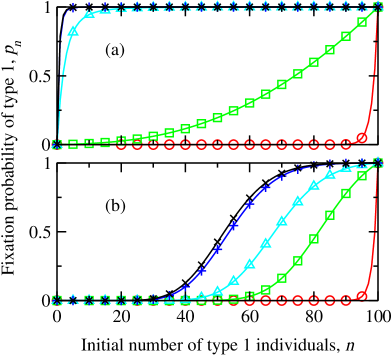
Figure 1: Fixation probabilities in the games (a) Harmony ($a=1$, $b=0.25$, $c=0.75$, $d=0.01$) and (b) Stag-Hunt ($a=1$, $b=0.01$, $c=0.8$, $d=0.2$), for $s$ equal to 1 ($\circ$), 5 ($\Box$), 10 ($\triangle$), 100 ($+$), or $\to\infty$ ($\times$). Note that, in figure (a), curves overlap for $s=10,100$ and $\to\infty$. Population size $N=100$.

For class II, a good paradigm is the Stag-Hunt game Skyrms (2003) ($a=1$, $b=0.01$, $c=0.8$, $d=0.2$), which is a coordination game: Strategy 1 maximizes the mutual benefit, whereas strategy 2 minimizes the risk of loss, and the conflict results from having to choose between these two options. As Fig. 1(b) reveals, the round-robin result is obtained for large $s$: both strategies are attractors, with the basin boundary located at the frequency corresponding to the mixed strategy equilibrium, i.e. $x=(d-b)/(a-c+d-b)\approx 0.49$. However, for small values of $s$ this boundary shifts to greater frequency values, thus reflecting an advantage of strategy 2. In the extreme $s=1$ case this strategy becomes the unique attractor.

It is interesting to note that Fig. 1 shows that there is not a general crossover at $s\approx N$. In the Harmony game, the round-robin regime is mostly reached for $s\simeq 10\ll N$, whereas in the Stag-Hunt game this does not happen until $s\simeq 100=N$.

Finally, let us consider the Snowdrift game Sugden (2004) ($a=1$, $b=0.2$, $c=1.8$, $d=0.01$) as an example of class III. This is also a dilemma game, as each player has to choose between strategy 1, which maximizes the population gain, and strategy 2, which gives individuals the maximum payoff by exploiting the opponent. With round-robin dynamics both strategies coexists in the long run, with frequencies corresponding to the mixed strategy equilibrium. However, our dynamics can never maintain coexistence indefinitely, because by construction one of the absorbing states (all players of type 1 or all of type 2) will be reached sooner or later with probability 1. Nonetheless, it is possible to study the duration of metastable states by using the mean time in each population state before absorbtion, $t_{n}$ Karlin and Taylor (1975). Figure 2 shows the results for two values of $s$ and a broad range of initial conditions. For $s$ large ($s=100$), the population stays for a long time near the value corresponding to the mixed strategy equilibrium $x=(d-b)/(a-c+d-b)\approx 0.19$, independently of the initial number of type 1 individuals. A smaller value of $s=10$ (not shown) induces a shift of the metastable equilibrium to smaller values of $n$, again almost independently of the initial conditions. Finally, for an even smaller value of $s$ ($s=5$), there is no metastable equilibrium, but a fluctuation towards the $x=0$ absorbing state, which clearly depends on the initial conditions.

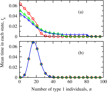
Figure 2: Mean time before fixation in the Snowdrift game ($a=1$, $b=0.2$, $c=1.8$, $d=0.01$), for $s$ equal to 5 (a) and 100 (b). Initial values of $n$ equal to 20 ($\circ$), 50 ($\triangle$) and 80 ($+$). Note that curves in (b) overlap. Population size $N=100$.

Having given examples of all three classes, we will summarize the rest of our study by saying that the remaining $2\times 2$ games behave in a similar way, with rapid selection (small $s$) favoring in all cases the type that has the greatest coefficient in the skew diagonal of the payoff matrix. For the remaining five games of class I this results in a reinforcement of the dominant strategy (the Prisoner’s Dilemma Axelrod and Hamilton (1981) being a prominent example). The other two games of class II exhibit once again a displacement of the basins of attraction, whereas the other two class III games display the suppression of the coexistence state in favor of one of the strategies. We thus see that rapid selection leads very generally to outcomes entirely different from those of round-robin dynamics.

It is important to realize that our results do not change qualitatively with the system size. Considering for instance the Stag-Hunt game, the change in the basins of attraction is practically independent of the population size. The main effect of working with larger sizes is a steeper transition between the basins of attraction. Indeed, due to the inherent stochasticity of finite population sizes, smaller populations have a more blurred basin boundary, with points in each basin having an increasing non-zero probability of reaching the other basin Cabrales (2000). Our results for all other symmetric $2\times 2$ games are equally robust. In fact, for very rapid selection, $s=1$, the limit $N\to\infty$ of the transition probabilities, Eq. (7), shows that they depend only on the frequencies of both types.

It could be argued that in our model only $s$ pairs of individuals play in each round, resulting in a very small effective population, this being the fundamental cause of the reported results. To probe into this issue, we have introduced a background of fitness Claussen and Traulsen (2005); Nowak et al. (2004), so that every player has an intrinsic probability of being selected, regardless of the outcome of the game, and thus guaranteeing a population of $N$ players. Indeed, in most applications, agents interact through more than one type of game and there are external contributions to fitness(environmental factors, fashions or media influence in a social context, etc.). Let $f_{b}$ be the normalized fitness background, so that each individual has a background of fitness $sf_{b}/N$ before selection takes place; $f_{b}=1$ means that the overall fitness coming from the game and from the background are approximately equal, for every value of $s$ and $N$. Figure 3 shows the results for the Stag-Hunt game. A small fitness background of $f_{b}=0.1$ gives fixation probabilities very similar to those with $f_{b}=0$ (Fig. 2(b)). For larger values, $f_{b}=1$, the displacement of the basin boundary is smaller, but still perfectly noticeable. And a very large fitness background, $f_{b}\gtrsim 10$ (not shown), drives the dynamics to random selection for every value of $s$, because in this case the influence of the game is almost negligible. Again, for the remaining symmetric $2\times 2$ games, our conclusions remain valid as well in the presence of a background of fitness. Consequently, our results are not merely due to a finite size effect of a small effective population of players.

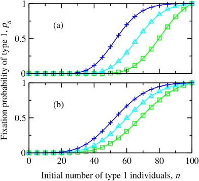
Figure 3: Fixation probability in the Stag-Hunt game ($a=1$, $b=0.01$, $c=0.8$, $d=0.2$) with a background of fitness $f_{b}$ equal to 0.1 (a) and 1 (b). Values of $s$: 5 ($\Box$), 10 ($\triangle$) 100 ($+$). Population size $N=100$.

In summary, we have proven that considering independent interaction and selection time scales leads to highly non-trivial, counter-intuitive results. We have demonstrated the generality of this conclusion by considering all symmetric $2\times 2$ games and showing that rapid selection may lead to changes of the asymptotically selected equilibria, to changes of the basins of attraction of equilibria, or to suppression of long-lived metastable equilibria. This result has major implications for applying evolutionary game theory to model a specific problem, as the assumption of slow selection and consequently of round-robin dynamics may or may not be correct. Indeed, as the example in Sánchez and Cuesta (2005) shows, rapid selection may lead to the understanding of problems where Darwinian, individual evolution was thought not to play a role because round-robin dynamics was used. We envisage that successful modelling in rapidly changing environments, such as social or (sub-)culture dynamics, will need a careful consideration of the involved time scales along the lines discussed here.

We thank R. Toral for a critical reading of the manuscript. This work is supported by MEC (Spain) under grants BFM2003-0180, BFM2003-07749-C05-01, FIS2004-1001 and NAN2004-9087-C03-03 and by Comunidad de Madrid (Spain) under grants UC3M-FI-05-007, SIMUMAT-CM and MOSSNOHO-CM.

References

- Maynard Smith (1982) J. Maynard Smith, Evolution and the Theory of Games (Cambridge University Press, 1982).
- Hofbauer and Sigmund (1998) J. Hofbauer and K. Sigmund, Evolutionary Games and Population Dynamics (Cambridge University Press, 1998).
- Camerer (2003) C. F. Camerer, Behavioral Game Theory (Princeton University Press, 2003).
- Szabó and Hauert (2002) G. Szabó and C. Hauert, Phys. Rev. Lett. 89, 118101 (2002).
- Traulsen et al. (2004) A. Traulsen, T. Röhl, and H. G. Schuster, Phys. Rev. Lett. 93, 28701 (2004).
- Zimmermann et al. (2004) M. G. Zimmermann, V. M. Eguíluz, and M. San Miguel, Phys. Rev. E 69, 65102 (2004).
- Claussen and Traulsen (2005) J. C. Claussen and A. Traulsen, Phys. Rev. E 71, 25101 (2005).
- Santos and Pacheco (2005) F. C. Santos and J. M. Pacheco, Phys. Rev. Lett. 95, 98104 (2005).
- Traulsen et al. (2005) A. Traulsen, J. C. Claussen, and C. Hauert, Phys. Rev. Lett. 95, 238701 (2005).
- Ariosa and Fort (2005) D. Ariosa and H. Fort, Phys. Rev. E 71, 16132 (2005).
- Hauert and Szabó (2005) C. Hauert and G. Szabó, Am. J. Phys. 73, 405 (2005).
- Hendry and Kinnison (1999) A. P. Hendry and M. T. Kinnison, Evolution 53, 1637 (1999).
- Hendry et al. (2000) A. P. Hendry, J. K. Wenburg, P. Bentzen, E. C. Volk, and T. P. Quinn, Science 290, 516 (2000).
- Yoshida et al. (2003) T. Yoshida, L. E. Jones, S. P. Ellner, G. F. Fussmann, and N. G. H. Jr., Nature 424, 303 (2003).
- Sánchez and Cuesta (2005) A. Sánchez and J. A. Cuesta, J. Theor. Biol. 235, 233 (2005).
- Moran (1962) P. A. P. Moran, The Statistical Processes of Evolutionary Theory (Clarendon Press, Oxford, 1962).
- Roughgarden (1979) J. Roughgarden, Theory of Population Genetics and Evolutionary Ecology: An Introduction (MacMillan Publishing Co., New York, 1979).
- Nowak et al. (2004) M. A. Nowak, A. Sasaki, C. Taylor, and D. Fudenberg, Nature 428, 646 (2004).
- Karlin and Taylor (1975) S. Karlin and H. M. Taylor, A First Course in Stochastic Processes (Academic Press, New York, 1975), 2nd ed.
- Rapoport and Guyer (1966) A. Rapoport and M. Guyer, General Systems 11, 203 (1966).
- Licht (1999) A. N. Licht, Yale J. Int. Law 24, 61 (1999).
- Skyrms (2003) B. Skyrms, The Stag Hunt and the Evolution of Social Structure (Cambridge University Press, 2003).
- Sugden (2004) R. Sugden, Economics of Rights, Co-operation and Welfare (Palgrave Macmillan, Hampshire, 2004), 2nd ed.
- Axelrod and Hamilton (1981) R. Axelrod and W. D. Hamilton, Science 211, 1390 (1981).
- Cabrales (2000) A. Cabrales, Int. Econ. Rev. 41, 451 (2000).