Probabilistic Regulatory Networks: modeling genetic networks

Abstract.

We describe here the new concept of $\epsilon$-Homomorphisms of Probabilistic Regulatory Gene Networks(PRN). The $\epsilon$-homomorphisms are special mappings between two probabilistic networks, that consider the algebraic action of the iteration of functions and the probabilistic dynamic of the two networks. It is proved here that the class of PRN, together with the homomorphisms, form a category with products and coproducts. Projections are special homomorphisms, induced by invariant subnetworks. Here, it is proved that an $\epsilon$-homomorphism for $0<\epsilon<1$ produces simultaneous Markov Chains in both networks, that permit to introduce the concepts of $\epsilon$-isomorphism of Markov Chains, and similar networks.

Introduction

We can understand the complex interactions of genes using simplified models, such as discrete or continuous models of genes. Developing computational tools permits description of gene functions and understanding the mechanism of regulation [7, 9]. We focus our attention in the discrete structure of genetic regulatory networks instead of continuous models. Probabilistic Gene Regulatory Network (PRN) is a natural generalization of the Probabilistic Boolean Network (PBN) model introduced in [8], and [2]. This model have $n$ functions defined over a finite set $X$ to itself, with probabilities assigned to these functions. We present here the ideas of $\epsilon$-similar networks, and isomorphism of Markov Chain. $\epsilon$-homomorphisms are used to describe subnetworks and similar networks, because they transform the discrete structure of one network to another, and the probability distributions of the networks are enough close, using a preestablished $0<\epsilon<1$ as a distance between the probabilities.

1. Preliminaries

Probabilistic Regulatory Networks A Probabilistic Gene Regulatory Network (PRN) (or a Probabilistic Dynamical Systems)[2] is a triple $\mathcal{X}=(X,F,C)$ where $X$ is a finite set and $F=\{f_{1},\ldots,f_{n}\}$ is a set of functions from $X$ into itself, with a list $C=(c_{1},\ldots,c_{n})$ of selection probabilities, where $c_{i}=p(f_{i})$, [2] We associate with each PRN a weighted digraph, whose vertices are the elements of $X$, and if $u,v\in X$, there is an arrow going from $u$ to $v$ for each function $f_{i}$ such that $f_{i}(u)=v$, and the probability $c_{i}$ is assigned to this arrow. This weighted digraph will be called the state space of $\mathcal{X}$. In this paper, we use the notation PRN for one or more networks. If $X=X_{1}\times\cdots X_{n}$ is the product of $n$ sets of possible values of the variables, then with the vector function $f=(f^{1},\cdots,f^{n})$ we associate a digraph $\Gamma$, called dependency graph, with vertex set $\{1,\dots,n\}$. There is a directed edge from $i$ to $j$ if $xi$ appears in the component function $f^{j}$. For a PRN, we have a dependency graph (dep-graph) for each function, then we superpose all the dep-graph and that is the low level digraph of our PRN [8]

Example. Suppose we have two genes with two values that we denote as usual $\{0,1\}$, that is this PRN is a very simple PBN. The set of boolean functions $F$ is the following:

$$F=\{f_{1}(x1,x2)=(x1,0),f_{2}(x1,x2)=(1,x2),$$

$$f_{3}(x1,x2)=(1,0),f_{4}(x1,x2)=(x1x2,x2)\},$$

and the probabilities are $\{.21,.22,.34,.23\}$. Therefore, the PBN $\mathcal{X}=(X,F,C)$ has the following state space, dependency graph, and transition matrix.

$$\begin{array}[]{c}\overset{.66}{\circlearrowright}(0,0)\leftarrow^{.21}(0,1)\circlearrowleft^{.23}\\ {}^{.34}\downarrow\uparrow^{.23}\hbox{ }\swarrow_{.34}\downarrow^{.22}\\ \overset{.77}{\circlearrowright}(1,0)\overset{.55}{\longleftarrow}(1,1)\circlearrowleft^{.45}\\ \hbox{ State space}\cr\end{array}\hskip 79.49744pt\begin{array}[]{c}{\curvearrowleft}\hskip 43.36243pt{\curvearrowleft}\\ \underline{\overline{|\textmd{gene \ 1}|}}\hskip 7.22743pt{\longleftarrow}\hskip 7.22743pt\underline{\overline{|\textmd{gene \ 2}|}}\\ \hbox{ Dependency graph}\\ \hbox{ of genes x1 and x2}\cr\end{array}$$

$$T=\left[\begin{array}[]{cccc}.66&0&.34&0\\ .21&.23&.34&.22\\ .23&0&.77&0\\ 0&0&.55&.45\cr\end{array}\right]$$

$\epsilon$-Homomorphisms of PRN. If $C$ is a set of selection probabilities we denote by $\chi$ the characteristic function over $C$. That is $\chi:C\cup\{0\}\rightarrow\{0,1\}$ such that $\chi(c)=1$, if $c\neq 0$ and $\chi(0)=0$. Let $\mathcal{X}_{1}=(X_{1},F=(f_{i})_{i=1}^{n},C)$ and $\mathcal{X}_{2}=(X_{2},G=(g_{j})_{j=1}^{m},D)$ be two PRN. A map $\phi:X_{1}\rightarrow X_{2}$ is an $\epsilon$-homomorphism from $\mathcal{X}_{1}$ to $\mathcal{X}_{2}$, if for a fixed real number $0\leq\epsilon<1$, and for all $f_{i}$ there exists a $g_{j}$, such that for all $u$, $v$ in $\mathcal{X}_{1}$,

(1) $\phi\circ f_{i}=g_{j}\circ\phi;$ (2) $max_{u,v}|c_{f_{i}}(u,v)-d_{g_{j}}(\phi(u),\phi(v))|\leq\epsilon$, and

(3) $\chi(d_{g_{j}}(\phi(u),\phi(v)))\geq\chi(c_{f_{i}}(u,v)).$

If $\phi:X_{1}\rightarrow X_{2}$ is a bijective map, and $d_{g_{j}}(\phi(u),\phi(v))=c_{f_{i}}(u,v)$, for all $f_{i}$, $g_{j}$, $u$, and $v$ in $\mathcal{X}_{1}$; then $\phi$ is an isomorphism.

If we denote by $p(u,v)=\sum_{f_{i}}c_{f_{i}}(u,v)$ and $p(\phi(u),\phi(v))=\sum_{g_{j}}d_{g_{j}}(\phi(u),\phi(v))$, then condition (2) implies that $|p(u,v)-p(\phi(u),\phi(v))|\leq k\epsilon$, where $k$ is the maximum number of functions going from one state to another in the network. So, if $T_{1}$ denote the transition matrix of $\mathcal{X}_{1}$, and the entry $(u,v)$ of $T_{1}$ is $p(u,v)$ then the third condition implies that: $max_{u,v}|({T_{1}})_{u,v}-({T_{2}})_{\phi(u),\phi(v)}|\leq k\epsilon$, for all possible $u$ and $v$ in $\mathcal{X}_{1}$.

2. Isomorphism of Markov Chains, $\epsilon$-Similar Networks

Two PRN are $\epsilon$-similar if there exists a bijective homomorphism $\phi$ between them, such that $\phi^{-1}$ is also an homomorphism. Observe that $\phi$ and $\phi^{-1}$ have the same $\epsilon$. When two PRN are $\epsilon$-similar, the two transition matrices have the a similar distribution of probabilities.

Theorem 2.1.

If $\phi:\mathcal{X}_{1}\rightarrow\mathcal{X}_{2}$, and $\phi^{-1}$ are bijective $\epsilon$-homomorphisms, then

max$|(c_{f^{m}}(u,f^{m}(u))-d_{g^{m}}(\phi(u),g^{m}(\phi(u)))|\leq m\epsilon$,

for all $m>2$; $u$, $v$, in $\mathcal{X}_{1}$.

Proof.

If $\chi(c_{f}(u,f(u)))=1$, then $\chi(d_{g}(\phi(u),\phi(f(u))))=1$, because $\phi$ and $\phi^{-1}$ are bijective homomorphisms. By definition of $\epsilon$-homomorphism, $g(\phi(u))=\phi(f(u))$. Then for $m=2$, and by the Chapman-Kolmogorov equation [10], we have the following:

$$|c_{f^{2}}(u,f^{2}(u))-d_{g^{2}}(\phi(u),g^{2}(\phi(u)))|=$$

$$|c_{f}(u,f(u))c_{f}(f(u),f^{2}(u))-d_{g}(\phi(u),g(\phi(u)))d_{g}(g(\phi(u)),g^{2}(\phi(u)))|=$$

$$|c_{f}(u,f(u))c_{f}(f(u),f^{2}(u))-d_{g}(\phi(u),\phi(f(u)))d_{g}(\phi(f(u)),\phi(f^{2}(u)))|\leq$$

By condition (2) in definition of homomorphism, we have

$$\leq|c_{f}(f(u),f^{2}(u))|\epsilon+|d_{g}(\phi(u),\phi(f(u)))|\epsilon\leq 2\epsilon.$$

Then we proved that $|c_{f^{2}}(u,f^{2}(u))-d_{g^{2}}(\phi(u),g^{2}(\phi(u)))|\leq 2\epsilon$.

Using this property, and mathematical induction over $m$, we can conclude that our claim holds. ∎

Corollary 2.2.

If $\phi:\mathcal{X}_{1}\rightarrow\mathcal{X}_{2}$, and $\phi^{-1}$ are bijective $\epsilon$-homomorphisms, then the transition matrices $T_{1}$ and $T_{2}$ satisfy the condition:

• $\chi(T_{1}^{m})_{u,v}=\chi(T_{2}^{m})_{\hat{u},\hat{v}}$,

• $\sum_{i=1}^{n}((T_{1}^{m})_{u,v}-(T_{2}^{m})_{\hat{u},\hat{v}})=0$,

for all $m$, $\hat{u}=\phi(u)$, and $\hat{u}=\phi(u)$.

An $\epsilon$-homomorphism between two PRN determines a correspondence between the Markov Chains of these two networks. Here, we introduce the concept of two similar Time Discrete Markov Chain (TDMC).

Definition 2.3.

Two TDMC of the same size $n\times n$: $\{T_{1},\ T_{1}^{2},\ T_{1}^{3},\ \ldots\}$, and $\{T_{2},\ T_{2}^{2},\ T_{2}^{3},\ \ldots\}$ are $\epsilon$-similar or $\epsilon$-isomorphic if there exists an $\epsilon\in\mathbb{R}$ small enough, such that $T_{1}^{m}-T_{2}^{m}=(t_{ij})_{n\times n}$ satisfies that

• $|t_{ij}|<\epsilon$, and $\sum_{i=1}^{n}t_{ij}=0$,

• $\chi(T_{1}^{m})_{ij}=\chi(T_{2}^{m})_{ij}$, for all $m$, where $\chi$ is the characteristic function.

That is, these two TDMC simulated the dynamic of two $\epsilon$-similar networks.

Example 2.4.

The networks with dynamic $T_{1}$ and $T_{2}$ are $.005$-similar. In fact

$$T_{1}=\left[\begin{array}[]{cccc}0&.549&.451&0\\ 0&.338&0&.662\\ .111&.445&.444&0\\ 0&.013&0&.987\cr\end{array}\right]T_{2}=\left[\begin{array}[]{cccc}0&.544&.456&0\\ 0&.337&0&.663\\ .113&.448&.439&0\\ 0&.011&0&.989\cr\end{array}\right]$$

Observe that,

$$T_{1}-T_{2}=\left[\begin{array}[]{cccc}0&.005&-.005&0\\ 0&.001&0&-.001\\ -.002&-.003&.005&0\\ 0&.002&0&-.002\cr\end{array}\right]$$

As a consequence, we obtain $max|(T_{1})_{ij}-(T_{2})_{ij}|\leq.005$, and both dynamics are .005-isomorphic. The steady state of $T_{1}$ is $\pi_{1}=(0,.01926,0,.98074)$, and the steady state of $T_{2}$ is $\pi_{2}=(0,.01632,0,.98368)$, [10]. We can see that $|\pi_{1}-\pi_{2}|=max_{i}|\pi_{1}(i)-\pi_{\phi}(i)|<.004$. Additionally, we have

$${T_{1}}^{2}-{T_{2}}^{2}=\left[\begin{array}[]{cccc}-.001467&-.00136&.00006&.00277\\ 0&.00199&0&-.00199\\ -.00232&-.00019&.00295&-.00243\\ 0&.002639&0&-.00263\cr\end{array}\right],$$

therefore $max|(T_{1}^{2})_{ij}-(T_{2}^{2})_{ij}|\leq.003$.

$$T_{1}^{3}-{T_{2}}^{3}=\left[\begin{array}[]{cccc}-.000394&-.00044&.00011&.00073\\ 0&.002525&0&-.00253\\ -.000161&.00156&.00213&-.00353\\ 0&.002843&0&-.002843\cr\end{array}\right],$$

and $max|(T_{1}^{3})_{ij}-(T_{2}^{3})_{ij}|\leq.004$. In the above example, the TDMC generated by $T$ and $T_{2}$ are $.005$-similar, and the networks simulated by them are $.005$-similar.

3. The category of Probabilistic Regulatory Networks, and mathematical background

For a $\epsilon\in\mathbb{R}$ small enough, we have the following theorem.

Theorem 3.1.

If $\phi_{1}:\mathcal{X}_{\rightarrow}\mathcal{X}_{2}$, and $\phi_{2}:\mathcal{X}_{2}\rightarrow\mathcal{X}_{3}$ are $\epsilon_{i}$-homomorphisms, for $i=1,2$. Then $\phi=\phi_{2}\circ\phi_{1}:\mathcal{X}_{1}\rightarrow\mathcal{X}_{3}$ is an $\epsilon$-homomorphism. Therefore the Probabilistic Regulatory Networks with the $\epsilon$-homomorphisms of PRN form the category PRN.

Proof.

The Probabilistic Regulatory Networks with the PRN homomorphisms is a category if: the composition is an homomorphism, and satisfy the associativity law; and there exists an identity homomorphism for each PRN.

(1) Let $\phi_{1}:\mathcal{X}_{1}\rightarrow\mathcal{X}_{2}$ be an $\epsilon_{1}$-homomorphism, and let $\phi_{2}:\mathcal{X}_{2}\rightarrow\mathcal{X}_{3}$ be an $\epsilon_{2}$-homomorphism. If $h\in\mathcal{X}_{3}$, $g\in\mathcal{X}_{2}$ and $f\in\mathcal{X}_{1}$ are functions in each PRN, and such that $\phi_{1}\circ f=g\circ\phi_{1}$ and $\phi_{2}\circ g=h\circ\phi_{2}$, then we will prove that: $\phi\circ f=h\circ\phi.$ In fact,

$$(\phi_{2}\circ\phi_{1})\circ f=\phi_{2}\circ(\phi_{1}\circ f)=\phi_{2}\circ(g\circ\phi_{1})=(\phi_{2}\circ g)\circ\phi_{1}=$$

$$(h\circ\phi_{2})\circ\phi_{1}=h\circ(\phi_{2}\circ\phi_{1}).$$

(2) To verify the second condition for $\epsilon$-homomorphism, we do the following. If $c_{f}(\phi(u),\phi(v))\neq 1$, with $u,\ v=f(u)\in X_{1}$, for some $f\in\mathcal{X}_{2}$,then we will prove that there exists an $\epsilon<1$ such that

$$|c_{f}(u,v)-t_{h}(\phi(u),\phi(v))|<\epsilon.$$

by part (1). We denote by $\hat{u}=\phi_{1}(u)$, $\hat{v}=\phi_{1}(v)$.

$$|c_{f}(u,v)-d_{g}(\phi_{1}(u),\phi_{1}(v))+d_{g}(\phi_{1}(u),\phi_{1}(v))-t_{h}(\phi_{2}(\hat{u}),\phi_{2}(\hat{v}))|\leq$$

$$|c_{f}(u,v)-d_{g}\phi_{1}(u),\phi_{1}(v)|+|d_{g}(\phi_{1}(u),\phi_{1}(v))-t_{h}(\phi_{2}(\hat{u}),\phi_{2}(\hat{v}))|\leq$$

Therefore our claim holds, $|c_{f}(u,v)-t_{h}(\phi(u),\phi(v))|<\epsilon_{1}+\epsilon_{2}.$

(3) We want to prove that $\chi(t_{h}(\phi(u),\phi(v)))\geq{\chi(c_{f}(u,v))}.$ Suppose that ${\chi(c_{f}(u,v))}=1$. Then, since $\phi_{1}$ is an homomorphism of PRN, we have that

$$\chi(d_{g}(\phi_{1}(u),\phi_{1}(v)))\geq{\chi(c_{f}(u,v))=1}$$

Since $\phi_{2}$ is an homomorphism of PRN, we obtain that

$$\chi(t_{h}(\phi(u),\phi(v)))=\chi(t_{h}(\phi_{2}(\phi_{1}(u)),\phi_{2}(\phi_{1}(v))))\geq\chi(c_{f}(\phi_{1}(u),(\phi_{1}(v))=1.$$

Therefore we have that $\chi(t_{h}(\phi_{2}(\phi_{1}(u)),\phi_{2}(\phi_{1}(v))))=1.$

Then the composition of two PRN-homomorphisms is an homomorphism.

The associativity and identity laws are easily checked, then our claim holds, and PRN is a category. ∎

For proofs of the following theorems see [3]

Theorem 3.2.

Let $\mathcal{X}_{1}\times\mathcal{X}_{2}=(X_{1}\times X_{2},H,E)$ be a product of PRN $\mathcal{X}_{1}=(X_{1},F,C)$ and $\mathcal{X}_{2}=(X_{2},G,D)$. If $\delta_{i}:X\rightarrow X_{i}$ are two PRN-homomorphisms, then there exists an homomorphism $\delta:X\rightarrow X_{1}\times X_{2}$, such that $\phi_{i}\circ\delta=\delta_{i}$ for $i=1,2$. That is, the following diagram commutes

$$\begin{array}[]{c}\hskip 3.61371ptX_{1}\times X_{2}\\ \overset{\phi_{1}}{\swarrow}\hskip 7.22743pt\overset{\delta}{\uparrow}\hskip 7.22743pt\overset{\phi_{2}}{\searrow}\\ X_{1}\overset{\delta_{1}}{\longleftarrow}X\overset{\delta_{2}}{\longrightarrow}X_{2}\cr\end{array}$$

This homomorphism is unique.

Theorem 3.3.

Let $\mathcal{X}_{1}\oplus\mathcal{X}_{2}=(X_{1}\times X_{2},H,E)$ be a product of PRN $\mathcal{X}_{1}=(X_{1},F,C)$ and $\mathcal{X}_{2}=(X_{2},G,D)$. If $\gamma_{i}:X_{i}\rightarrow X$ are two PRN-homomorphisms, then there exists an homomorphism $\gamma:X_{1}\oplus X_{2}\rightarrow X$, such that $\gamma\circ\iota_{i}=\gamma_{i}$ for $i=1,2$. That is, the following diagram commutes

$$\begin{array}[]{c}\hskip 3.61371ptX_{1}\oplus X_{2}\\ \overset{\iota_{1}}{\nearrow}\hskip 7.22743pt\overset{\gamma}{\downarrow}\hskip 7.22743pt\overset{\iota_{2}}{\nwarrow}\\ X_{1}\overset{\gamma_{1}}{\longrightarrow}X\overset{\gamma_{2}}{\longleftarrow}X_{2}\cr\end{array}$$

This homomorphism is unique.

4. Subnetworks

A subnetwork $Y\subseteq X$ of $\mathcal{X}=(X,F,C)$ is an invariant subnetwork or a sub-PRN of $\mathcal{X}$ if $f_{i}(u)\in Y$ for all $u\in Y$, and $f_{i}\in F$. Sub-PRNs are sections of a PRN, where there aren’t arrows going out. The complete network $X$, and any cyclic state with probability 1, are sub-PRNs. An invariant subnetwork is irreducible if doesn’t have a proper invariant subnetwork. An endomorphism is a projection if $\pi^{2}=\pi$.

Theorem 4.1.

If there exists a projection from $\mathcal{X}$ to a subnetwork $\mathcal{Y}$ then $\mathcal{Y}$ is an invariant subnetwork of $\mathcal{X}$.

Proof.

Suppose that there exists a projection $\pi:X\rightarrow Y$. If $y\in Y$, by definition of projection $\pi(y)=y$, and $f_{i}(\pi(y))=\pi(g_{j}(y))$. Therefore all arrows in the subnetwork $Y$ are going inside $Y$, and the network is invariant. ∎

4.1. Constructing a PRN with real data

Here we developed a method to construct a PRN. In this case, we suppose that the information given by the experiment is a dependency graph and a time series data, see Figure 1, and Table 1.

$f_{1}$-data	3	6	9	12
x1	2	2	2	2
x2	1	0	0	0
x3	0	1	0	0

$f_{2}$-data	3	6	9	12
x1	1	1	1	1
x2	0	1	0	0
x3	1	0	0	0

$f_{3}$-data	3	6	9	12
x1	2	0	0	0
x2	0	0	0	0
x3	1	1	1	1

Table 1. Time series data

Additionally, we know that this information is noisy, and the first gene has three values, meanwhile the other two genes take only two $\{0,1\}$, so $X=\{0,1,2\}\times\{0,1\}^{2}$.

To determine the partially defined functions: $f_{1},\ f_{2},\ f_{3}$ over the finite field with $3$ elements ${\mathbb{Z}}_{3}$, we use the algorithm introduced in [4]. That is: the first variable $x1\in{\mathbb{Z}}_{3}$, meanwhile the other two genes $x_{2},$ and $x_{3}$ are in ${\mathbb{Z}}_{2}$.

For example with the first function $f_{1}=(f_{11},f_{12},f_{13})$ we do the following. We represent the functions with polynomials over the variables given by the dependency graph, and the operations $+$ and $\cdot$ are the usual in the finite field ${\mathbb{Z}}_{3}$. Then, the second component function

$$f_{12}(x1,x2,x3)=a+bx1+cx2+dx3+ex1x2+gx1x3+hx2x3+tx1x2x3$$

takes the following table of values. $f_{12}$ (mod 2) 1 0 0 0 x1 2 2 2 2 x2 1 0 0 0 x3 0 1 0 0 . Evaluating, we obtain the following linear system, where “=” means congruence (mod 2):

$$\left\{\begin{array}[]{rl}a+2b+c+2e&=0\\ a+2b+d+2g&=0\\ a+2b&=0\cr\end{array}\right..$$

Then reducing modulo 2, we have $a=c=d=0$, and $b,\ e,\ g,\ h,\ t,$ are free variables. So, one of the solution is $f_{12}=x1(1+x2+x3+x2x3),$ (mod 2). Using this method, we obtain the following functions:

$$\begin{array}[]{rl}f_{1}(x1,x2,x3)&=(x_{1},x1(1+x2+x3+x2x3),x_{2}),\\ f_{2}(x_{1},x_{2},x_{3})&=(x1,x3,0),\\ f_{3}(x_{1},x_{2},x_{3})&=(x1x2,x2,x3),\cr\end{array}$$

and they have the probabilities $c_{1}=.23,\ c_{2}=.34,\ c_{3}=.43$.

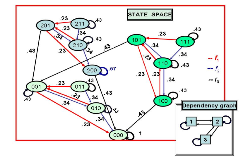
Figure 1. State Space of $\mathcal{G}$

The state space of $\mathcal{G}=(X,F,C)$ is in Figure $1$. The network has $12$ states.The only fixed point is $(0,0,0)$, and the state space has two subnetworks of 8 elements and one subnetwork of 4 elements. For each subnetwork we must have a projection. That is, an $\epsilon$-homomorphism $\pi:X\rightarrow Y$, must exist for each subnetwork $Y$. That is, the converse of the Theorem 4.1 could be true in some cases or with some little changes.

In particular, for the sub-PRN $\mathcal{Y}_{1}=\{Y_{1};F;C\}$ with

$$Y_{1}=\{(1,0,0),(1,0,1),(1,1,0),(1,1,1),(0,0,0),(0,0,1),(0,1,0),(0,1,1)\},$$

a projection $\pi_{1}:X\rightarrow Y_{1}$ exists, in fact: $\pi_{1}(x1,x2,x3)=(x1,x2,x3)$ if $x1=0,1$; and $\pi_{1}(x1,x2,x3)=(0,x2,x3)$ if $x1=2$. With this projection, it is possible to consider the first gene with only two values: $\{0,1\}$.

For the sub-PRN $\mathcal{Y}_{2}=\{Y_{2};F;C\}$ with

$$Y_{2}=\{(2,0,0),(2,0,1),(2,1,0),(2,1,1),(0,0,0),(0,0,1),(0,1,0),(0,1,1)\},$$

a projection $\pi_{2}:X\rightarrow Y_{2}$ doesn’t exist, because the first function $f_{1}$. So, taking a subnetwork of the whole PRN but without the function $f_{1}$ and a new assignation of probabilities we have a new PRN $\overline{\mathcal{G}}=\{X;f_{2},f_{3};d_{2},d_{3}\}$ and a projection $\pi_{2}:\overline{\mathcal{G}}\rightarrow\overline{\mathcal{Y}_{2}}$ exists, and it is given by: $\pi_{2}(x1,x2,x3)=(x1,x2,x3)$ if $x1=0,2$; and $\pi_{2}(x1,x2,x3)=(0,x2,x3)$ if $x1=1$, where $\overline{\mathcal{Y}}_{2}=\{Y_{2};f_{2},f_{3};d_{2},d_{3}\}$ The projections $\pi_{i}$ are $.57$-homomorphisms. These two subnetworks $\overline{\mathcal{Y}}_{1}$ and $\overline{\mathcal{Y}_{2}}$ are not similar.

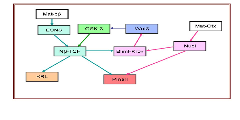
Figure 2. Mat-Act Dependency graph

4.2. Future work

The construction of a mathematical model for the genetic regulatory network ENDOMESODERM GENE NETWORK, described in [5, 6], will be developed in the future. The subnetwork, “Mat-Act” is formed with the action of two genes called: Mat-c$\beta$ and Mat-Otx over eight genes: ECNS, GSK3, Wnt8, N$\beta$-TCF, Bliml-Krox, Nucl, KRL, Pmarl; whose interaction is during 21 hours. We will use the above methodology, for the genetic network with the dependency graph in Figure 2, obtained in Biotapestry [6].

5. Acknowledgements

This research was supported by the National Institute of Health, PROGRAM SCORE, 2004-08, 546112, University of Puerto Rico-Rio Piedras Campus, IDEA Network of Biomedical Research Excellence, and the Laboratory Gauss University of Puerto Rico Research. The first author wants to thank Professor E. Dougherty for his useful suggestions, and Professor O. Moreno for his support during the last four years.

References

- [1]
- [2] M. A. Aviñó,and O. Moreno, “Homomorphisms of Probabilistic Gene Regulatory Networks”, Poster and Proceedings of GENSIPS 2006.
- [3] M. A. Aviñó, “A Probabilistic Gene Regulatory Networks, isomorphisms of Markov Chains”, http://arxiv.org/abs/math/0603302, 2006.
- [4] M. A. Aviñó, E. Green, and O. Moreno, “Applications of Finite Fields to Dynamical Systems and Reverse Engineering Problems” Proceedings of ACM Symposium on Applied Computing,(2004). (2004)
- [5] Eric H. Davidson et al., “A Genomic Regulatory Network for Development”. Science 295 (5560): 1669-1678, 2002
- [6] Eric H. Davinson, Davincson Laboratory,“ Bio Tapestry interactive network” http://sugp.caltech.edu/endomes/index.html
- [7] E. R. Dougherty, A. Datta, and C. Sima, “Developing therapeutic and diagnostic tools”, Research Issues in Genomic Signal Processing, IEEE Signal Processing Magazine [46-68] Nov. 2005.
- [8] I. Shmulevich, E. R. Dougherty, and W. Zhang, “From Boolean to probabilistic Boolean networks as models of genetic regulatory networks”, Proc. of the IEEE. 90(11): 1778-1792.(2001)
- [9] R. Somogyi and L.D. Greller, The dynamics of molecular networks: Applications to therapeutic discovery, Drug Discov. Today, vol. 6, no. 24, pp. 1267 1277, 2001.
- [10] J. W. Steward, “Introduction to the numerical solution of Markov Chain”, Princenton University Press, 1994.