A toy model of polymer stretching

Abstract

We present an extremely simplified model of multiple-domains polymer stretching in an atomic force microscopy experiment. We portray each module as a binary set of contacts and decompose the system energy into a harmonic term (the cantilever) and long-range interactions terms inside each domain. Exact equilibrium computations and Monte Carlo simulations qualitatively reproduce the experimental saw-tooth pattern of force-extension profiles, corresponding (in our model) to first-order phase transitions. We study the influence of the coupling induced by the cantilever and the pulling speed on the relative heights of the force peaks. The results suggest that the increasing height of the critical force for subsequent unfolding events is an out-of-equilibrium effect due to a finite pulling speed. The dependence of the average unfolding force on the pulling speed is shown to reproduce the experimental logarithmic law.

I Introduction

The last decade has witnessed a significant advancement of single molecule manipulation and visualization techniques Review-1 ; Review-2 ; Review-3 ; Review-4 ; Review-5 ; Review-6 ; Review-7 providing access to the distribution of physical properties across many individual molecules and not just average properties as was the case of traditional biochemical techniques.

Optical Tweezers (OT) and Atomic Force Microscopy (AFM) in particular, enable the study of mechanical properties of proteins such as those in the extracellular matrix, in the cytoskeleton and in the muscle, that in vivo are exposed to stretching forces. The mechanical properties of macromolecules obtained in these experiments may be directly connected to corresponding thermodynamical quantities bustamante with a bit of caution, since mechanical experiments are usually out-of-equilibrium, as discussed in this paper. On the other hand, the mechanical properties of biomolecules may be of direct importance for what concerns bendability (DNA), translocation of nucleic acids and proteins across cellular membranes, rigidity and elasticity (structural proteins).

In a force-measuring AFM experiment, the tip of a microscopic cantilever is pressed against a flat, gold-covered substrate, coated with a thin layer of protein. Upon retraction of the substrate, a protein molecule that may have been adsorbed to the cantilever tip is then stretched. Finally, the force the protein opposes to the stretching is computed from the cantilever deflection, and a force-extension plot is drawn. In a typical stretching experiment the force-extension curve shows a saw-tooth pattern, each peak corresponding to the unfolding of a single domain. However, if the protein is composed by several different modules, it is difficult to associate each peak to the corresponding domain. Moreover, in order to neglect the tip-substrate interaction, it is necessary to have a sufficiently long protein. A common strategy proposed in the literature to address these problems is to use an engineered protein composed by several tandem repeats of the same kind of domain. A typical choice is to use domains belonging to the immunoglobulin Ig , fibronectin III FN-III or cadherin cadherin superfamilies, characterized by $\beta$-sandwich structures. Alpha-helical domains, such as those of the cytoskeletal protein spectrin spectrin , have also been used.

Many data about the mechanical properties of modular proteins can be extracted from the force-extension profiles. The amplitude of each peak, in fact, represents the mechanical stability of the corresponding domain, while the spacing between peaks reflects the length of the unfolded domain and is thus proportional to the number of amino-acids it comprises. The experimental data also show a logarithmic dependence of the height of the peaks on the pulling velocity, so that higher forces are required for domain unraveling when the pulling occurs very quickly.

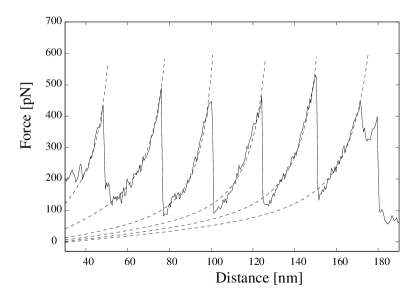
Figure 1: The force-extension profile produced in a typical AFM stretching experiment performed on a modular polyprotein composed by 8 tandem repetitions of a Ig-like domain from titin. The construct is terminated by 2 cystein residues expressly introduced to form covalent bonds with a gold surface. The experiment was performed at a constant speed of $200\mathrm{n}\mathrm{m}\mathrm{/}\mathrm{s}$. Notice that only 7 unfolding peaks appear in the plot because the cantilever tip, by chance, established a contact with the second domain of the molecule, skipping the first one.

The features of the force-extension curves (Figure  1) are accounted for by the entropic elasticity of polymer chains in solution. The entropy of a polymer, in fact, is maximal in the random coil state, whereas it tends to zero in the fully extended conformation. The force required to stretch a polymer thus reflects the entropy loss and it grows in a non-linear way as the molecule is lengthened. The entropic elasticity of biopolymers is currently modeled through the worm-like chain (WLC) WLC and freely-jointed chain (FJC) FJC models. The WLC model describes a molecular chain as a deformable rod whose stiffness is determined by the persistence length $p$ (the length scale over which the polymer loses orientation order). The functional relation between the external force and the fractional extension $z/L$ ($z$ is the end-to-end distance and $L$ is the contour length) is approximatly given by the interpolating formula

$$F=\frac{k_{B}T}{p}\left(\frac{1}{4(1-z/L)^{2}}-\frac{1}{4}+\frac{z}{L}\right),$$ (1)

where $k_{B}$ is the Boltzmann constant and $T$ is the temperature.

In the FJC model, the polymer is portrayed as a chain of rigid segments linked by frictionless joints so that each segment can point in any direction irrespective of the orientations of the others. A measure of the stiffness of the chain is represented by the Kuhn segment length $b$ (the average length of the segments). The analytic relation between the average end-to-end distance $\langle z\rangle$ and the stretching force $F$ is

$$\langle z\rangle=L\left(\coth\frac{Fb}{k_{B}T}-\frac{k_{B}T}{Fb}\right).$$ (2)

In our model, the polymer is described by an array of binary variables representing native contacts that can be in either of two states: formed or broken. The cantilever, on the other hand, is modeled as a harmonic spring in series with the molecule. The energy of the system is the sum of a harmonic term and a term of long-range interaction modeling in a bulk, coarse-grained way, the chemical interactions stabilizing the native conformation of the protein. In fact, rather than providing a detailed description, we account for chemical interactions through a folding prize attributed to a domain when the fraction of intact contacts is above a threshold. We assume any contact breakdown to produce an equal increment in the molecule length.

Let us consider first the force-extension characteristic of our model in the absence of folding prize. Let $F$ be a constant pulling force, $n$ the number of broken contacts and $a$ the length increment per cleaved contact. If no folding prize is attributed to the molecule in a native-like state, the Hamiltonian of the system is $\mathcal{H}=-Fna$ and the partition function is

$$Z=\sum_{n}\left(\begin{array}[]{c}N\\ n\end{array}\right)e^{\beta Fna}=(1+e^{\beta Fa})^{N}.$$

Notice that this is also the partition function of an Ising-like model in one dimension without coupling among spins. The average end-to-end distance can thus be computed as

$$\langle z\rangle=a\langle n\rangle=\frac{k_{B}T}{Z}\frac{\partial Z}{\partial F}=\frac{Na}{2}\left(1+\tanh\left(\frac{Fa}{2k_{B}T}\right)\right).$$ (3)

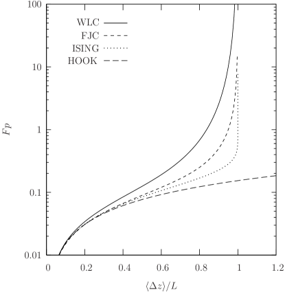
Figure 2: Force versus extension for various models: WLC (interpolated formula) with $p=0.4~{}\mathrm{n}\mathrm{m}$, $L=29~{}\mathrm{n}\mathrm{m}$, $T=310~{}\mathrm{K}$; FJC with $b=2p$, ISING with $a=1.3p$ $N=L$, HOOK (harmonic potential) with $K=1.3p$.

The variation of length $\langle\Delta z\rangle$ versus $F$ in the WLC, FJC and our (ISING) models is shown in Figure 2, where we have adjusted the constant $a$ (corresponding to persistence length $p$ so to make the curve coincide for small elongations. Despite the extreme simplicity of our assumptions, the three curves are qualitatively similar. This similarities could be increased by adding contact-contact interactions or considering different elongations for the various contact breaking events.

Although the WLC and FJC models more accurately represent the physics of a polymer, their statistical mechanics treatment is so complex that one generally employes the average formulas (1) and (2) for each domain, complemented with an independence hypothesis of domains and an ad-hoc treatment of the unfolding event Evans-1 ; Evans-2 ; Rief , based on an extension of Bell’s expression Bell or full Kramer’s theory Schlierf for the rupture rate coefficient in the presence of a time-dependent external force.

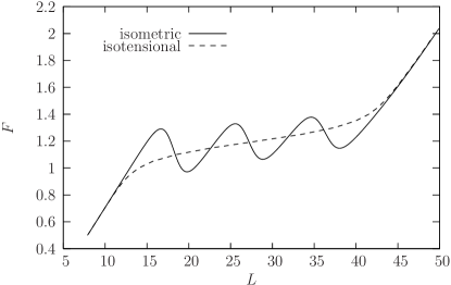
Figure 3: Isometric versus isotensional elongations for $M=3$, $A=1$, $K=0.1$, $N=10$, $\theta=0.2$ and $beta=2$ (see Section II for the illustration of the model).

The independence assumption is questionable, since all domains are coupled by the presence of the cantilever. This difference may be explicited by comparying computations bleha in which the position of the cantilever is observed (isometric) while the force may fluctuate, with computations in which the force is maintained constant (isotensional). We can obtain exact comparisons of the two different set-up for our model (see Section II), as shown in Figure 3. It can be noticed that the isotensional model does not show any peaks (the peaks are here smoothed due to the small length of the single module).

Moreover, the peaks in the force-extension profile (Fig. 1) are a signature of a first-order transition. As we shall show in the following, this transition naturally arise in our model due to the long-range coupling (the folding prize).

Despite its extreme simplicity, our approach captures some important aspects of the physics of Ig domain stretching. Steered molecular dynamics simulations performed in Schulten’s group Schulten1 ; Schulten2 ; Schulten3 , in fact, showed that the mechanical unfolding of the I27 module occurs only after the breakdown of a patch of six hydrogen bonds bridging the $A^{\prime}$ and $G$ $\beta$-strands. The rupture of these critical bonds was shown to be the key event allowing the full unraveling of the molecule under an external force.

Even if this pattern was originally observed in a specific protein, it could be hypothesized a more widespread distribution. Makarov and coworkers Makarov performed Monte Carlo simulations of titin forced unfolding. During these simulations the number of hydrogen bonds at time $t$, $n(t)$, undergoes a random walk. It was concluded that a critical value $n^{\#}$ of the number of hydrogen bond does exist, such that when $n(t)<n^{\#}$, the domain unfolds very rapidly. Makarov also showed that the number of bonds is roughly one, when the force is low enough, whereas for very large pulling rates (and thus large pulling forces), it is likely to be equal to six, recovering the findings by Lu and Schulten Schulten3 .

The accuracy of the model developed by Makarov and coworkers, allows quantitative comparisons with experimental data at the expense of very long simulation times and the need to assume the knowledge of the free energy profile. Their model is also based on the hypothesis of independence of domains which, however, might be incompatible with the coupling introduced by the cantilever. Since the transitions shown in AFM experiments are out of equilibrium Rief ; Grubmuller , thermal fluctuations may play a fundamental role. Our model, conversely, is so simplified that we can compute exactly the free energy of a multi-domain protein for the equilibrium case, and perform long simulations in the out of equilibrium case.

The model we propose shows interesting similarities to a Gō model with force rescaling. Recent theoretical studies Chan ; Cecconi show that the ability of Gō models to simulate the cooperativity of the folding process can be enhanced by imparting an extra energetic stabilization to the native state so as to simulate specific interactions appearing only after the assembly of native-like structures. A rigorous approach to simulate the stabilizing interactions peculiar of the native state, would be the use of two different analytic expressions of the force-field inside and outside the native basin. The same purpose can be pursued through a much simpler strategy Chan , by rescaling the conformational force when the fraction of native contacts crosses a pre-chosen threshold.

This approach appears to be similar to the one employed in our model. The energy function of our model comprises an elastic term and a contact term. The harmonic term accounts for the elasticity of the cantilever, while the protein can be thought of as a soft spring so that its contribution to the elasticity of the system is negligible.

The contact term of our energy function, on the other hand, is a stabilizing contribution that the protein receives only when the fraction of intact contacts crosses a threshold. This approach is thus equivalent to a force rescaling occurring whenever the polymer enters the native basin, and the contact term of the energy function appears to be a square well.

Finally, from a purely formal point of view, our description of the polymer as an array of binary variables, bears some similarity with the model proposed by Galzitskaya and Finkelstein (GF) Finkelstein . In the GF model, in fact, each residue of the polypeptide chain can be either in an ordered (native) or disordered (non-native) state, encoded by the two possible values of a binary variable. This approach, similarly to ours, significantly narrows the conformational space, that consists of $2^{N}$ conformations only, for a polymer with $N$ residues. This approach, while drastically reducing the computation time, is in agreement with the Zimm-Bragg model Zimm , widely employed to describe the helix-coil transition in heteropolymers.

The outline of the paper is as follows. In Section II we describe the model and the simulation procefdure; in Section III.1 we study the equilbrium behavio r of a single domain; in Section III.3 we investigate the role of fluctuations in the reciprocal influence between successive unfolding events; in Section III.4 we investigate the dependence of the unfolding force on the pulling rate and we sketch a simple analytic treatment of the unfolding probability in the limit of an extremely high pulling rate; finally, in Section IV we draw the conclusions of our work.

II The model

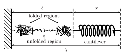
Figure 4: Schematic description of the AFM experimental set-up. The polymer is composed by several tandem repeats of the same domain in series with a harmonic spring (the cantilever).

The AFM in its simplest arrangement is just a spring (the cantilever) whose deflection, and thus the applied force, is measured as a function of its position. The system, as shown in Figure 4, can therefore be modeled as a harmonic spring in series with a protein composed by $M$ tandem repeats of the same domain. Each domain $j$ is simply portrayed as a sequence of contacts ($\boldsymbol{s}^{(j)}=\{s_{i}^{(j)}\}$, $i=1,\cdots,N$) that can be either intact ($s_{i}^{(j)}=0$) or broken ($s_{i}^{(j)}=1$), where $N$ is the total number of native contacts inside each domain. The length of the polymer chain can be simply computed as $\ell=\sum_{j=1}^{M}\sum_{i=1}^{N}s_{i}^{(j)}a=\sum_{j=1}^{M}an_{j}$, where $a$ represents the incremental elongation associated to each contact breakdown and $n_{j}=\sum_{i=1}^{N}s_{i}^{(j)}$ is the number of broken contacts in domain $j$. For the sake of simplicity, in all our computations we set $a=1$. The length of the spring, on the other hand, is just $x=\lambda-\ell$ where $\lambda$ is the extension of the spring-polymer system, using the rest position as the reference point.

The energy of a domain configuration $\boldsymbol{s}^{(j)}$ is modeled by the sum of two contributions: a harmonic term $H$, accounting for the presence of the spring, and the sum over all domains $j$ of a term $L^{(j)}$, related to the long-range interactions among the monomers,

$$E=H+\sum_{j=1}^{M}L^{(j)}.$$

The harmonic term is expressed as

$$H(x)=\frac{1}{2}Kx^{2}=\frac{1}{2}K(\lambda-\ell)^{2}=\frac{1}{2}K\left(\lambda-a\sum_{j=1}^{M}n_{j}\right)^{2},$$

where $K$ is the harmonic constant.

In our simplified representation, if the fraction of intact contacts $n_{j}/N$ in a domain $j$ is below a given threshold $\theta$, the domain receives a folding prize $AN$ proportional to the number of possible contacts. The interaction term is thus computed as

$$L^{(j)}=-AN\Theta(\theta N-n_{j}),$$

where $\Theta(x)$ is the Heaviside step function

$$\Theta(x)=\left\{\begin{array}[]{ll}0&\mbox{if $x<0$}\\ 1&\mbox{otherwise}\end{array}\right.$$

In summary, the energy of a configuration is just a function of the number of broken contacts in each domain

$$E(\boldsymbol{n})=\frac{1}{2}K[x(\boldsymbol{n})]^{2}-AN\Theta(\theta N-n_{j}),$$

where $\boldsymbol{n}=\{n_{1},n_{2},\ldots,n_{M}\}$ and

$$x(\boldsymbol{n})=\left(\lambda-a\sum_{j=1}^{M}n_{j}\right).$$

This assumption speeds up the computations, that may be performed in terms of the $n_{j}$.

A stretching simulation starts from a completely folded initial structure, where no contact is broken. The protein-spring length $\lambda$, chosen as the control parameter, is linearly increased from $\lambda_{Min}$ to $\lambda_{Max}$ in $k_{\lambda}+1$ steps during the simulation;

$$\lambda(k)=\lambda_{Min}+\frac{\lambda_{Max}-\lambda_{Min}}{k_{\lambda}}k,$$

where $k=0,1,\cdots,k_{\lambda}$. For each value of $\lambda$, we compute the average length of the spring $\langle x\rangle$ in an equilibrium simulation as

$$\langle x\rangle=\frac{1}{Z}\sum_{\boldsymbol{n}}g(\boldsymbol{n})\;x(\boldsymbol{n})e^{-\beta E(\boldsymbol{n})},$$

where $Z$ is the partition function

$$Z=\sum_{\boldsymbol{n}}g(\boldsymbol{n})e^{-\beta E(\boldsymbol{n})},$$

and the multeplicity factor

$$g(\boldsymbol{n})=\prod_{j=1}^{M}\binom{N}{n_{j}}$$

is given in terms of the number of possible microscopic configurations containing $n_{j}$ cleaved contacts.

In real stretching experiments, however, the polymer is subjected to a finite pulling velocity, so that the molecule cannot be considered in an equilibrium condition. In order to consider this effect, we use Monte Carlo simulations. For each value of $\lambda$, $T$ Monte Carlo steps are performed, each involving $N\times M$ elementary steps. The elementary step consists in the random choice of a domain and in the attempt to increase or decrease by one the number of contacts with probability equal to the fraction of broken or intact contacts respectively. The trial move is then accepted or rejected with a probability derived from the heat-bath criterion,

$$p(n_{j}\rightarrow n_{j}\pm 1)=\frac{e^{-\beta E(n_{1},\dots,n_{j}\pm 1,\dots,n_{M})}}{e^{-\beta E(n_{1},\dots,n_{j}+1,\dots,n_{M})}+e^{-\beta E(n_{1},\dots,n_{j}-1,\dots,n_{M})}},$$

where $\beta$ is the inverse temperature.

The average length of the spring $\langle x\rangle$, corresponding to the current position $\lambda$ is computed averaging over $T$ Monte Carlo steps.

III Results

We first analyze the entropic effects related to temperature through the analysis of computations in the absence of a folding prize, and then investigate the role of long-range interaction by setting a non-zero prize on a single-domain polymer. After that, we discuss a set of computations on a three-domain protein, showing the importance of the coupling due to the cantilever in the mechanism of mechanical unfolding and, in particular, they explain how the first unfolding event affects the following ones. In the last part, we discuss the relation between pulling rate and unfolding force, finding a logarithmic law. The section is completed with a analytic treatment of the unfolding probability valid in the limit of high pulling rate.

$N$ :	Maximum number of contacts per domain
$M$ :	Number of domains
$L$ :	Maximal length of the polymer-spring system
$k_{\lambda}$ :	Number of steps in the length of the polymer-spring system
$T$ :	Number of Monte Carlo steps
$A$ :	Folding prize (in units $N$)
$\theta$ :	Threshold to keep the folding prize
$K$ :	Elastic constant of the cantilever spring
$\beta$ :	Inverse temperature

Table 1: Legend of the symbols appearing in the figures.

The legend of the symbols appearing in the figures is shown in Table 1.

III.1 Single domain analysis

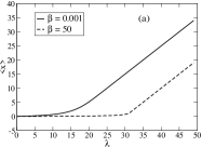
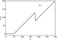
Figure 5: Cantilever deflection (force) versus estension for a single domain. (a) No folding price. Influence of temperature-dependent entropic effects on mechanical unfolding. Simulation parameters: $N=30$; $M=1$; $L=50$; $k_{\lambda}=50$; $A=0$; $K=0.1$; $\beta=0.001$ (solid line); $\beta=50$ (dashed line). (b) Typical ramp-like profile with folding prize. Simulation parameters: $N=100$; $L=300$; $k_{\lambda}=100$; $A=5$; $\theta=0.5$; $K=0.1$; $\beta=2$.

The force-extension curves without folding prize, as shown in Figure 5 (a), are clearly bi-phasic. The flat part of the curve at low temperature ($\beta=50$) represents the complete unfolding of the protein while the spring nearly retains its resting length: at low temperatures, the enthalpic contribution of the free energy (the harmonic energy of the cantilever), dominates over the entropic one. When the protein is completely stretched, the system can react to the increase of the control parameter $\lambda$, only through an equal increase of the spring length. The steep part of the $(x,\lambda)$ plot is thus a straight line with unitary slope.

At high temperature ($\beta=0.001$) the free energy is dominated by the entropic term so that for small values of $\lambda$, about $50\%$ of the monomers are extended in the direction of the pulling force so as to maximize entropy, while the spring remains in its resting position. The proportion of unfolded monomers remains thereafter almost unchanged during the simulation and for $\lambda>15$, any further increase in $\lambda$ is reflected in a equal extension of the spring $\Delta x=\Delta\lambda$.

III.2 Effect of folding prize

The protein is here composed by a single domain with $N=100$ contacts, and its energy is lowered by $A=5N$ when a fraction of residues greater than $\theta=0.5$ is folded.

The $(x,\lambda)$ plot portrayed in Figure 5 (b) shows a flat region for $\lambda\leq 50$. This reflects the cleavage of $N\times\theta=50$ contacts that can occur without the loss of the folding prize, while the spring remains very close to the resting length. As the further extension of the protein would result in a significant destabilization of the system due to the loss of the folding prize, the increase of the control parameter $\lambda$ is now completely accounted for by the stretching of the spring. The second part of the $(x,\lambda)$ plot is thus a straight line with unit slope. When the increase in harmonic energy exceeds the folding prize, the stretching of the spring is interrupted and the remaining 50 contacts of the protein break down, allowing a corresponding shortening of the spring. As the protein is now completely extended, any further increase in $\lambda$ must result in a corresponding stretching of the cantilever and the final part of the $(x,\lambda)$ plot is again a straight line with unit slope.

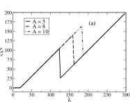
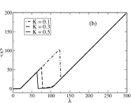
Figure 6: Role of folding prize $A$ (a) and harmonic constant $K$ (b). Common computation parameters: $N=100$; $M=1$; $L=300$; $k_{\lambda}=100$; $\theta=0.20$; $\beta=2$.

The features of the saw-tooth $(x,\lambda)$ profile are affected by several simulation parameters. The folding prize $A$ is related to the enthalpic component of the free energy and stabilizes the folded conformation of the protein. As a consequence, when $A$ is large, the polymer tends to remain in the compact conformation so as to retain the significant folding prize and the increase in $\lambda$ leads to a stretching of the cantilever spring. Only when $\langle x\rangle$ is very large it becomes enthalpically favourable for the polymer to unfold because the decrease in harmonic energy due to the cantilever relaxation more than compensates the loss of the folding prize. Thus, as $A$ is increased, higher and higher values of $\langle x\rangle$ are required for the elastic energy to compensate the folding prize and the peak of the $(x,\lambda)$ plot becomes accordingly higher and higher. The harmonic constant $K$ of the cantilever spring plays a role basically opposite to that of the folding prize. In fact, when $K$ is large, smaller average extensions $\langle x\rangle$ are required for the harmonic energy to balance the folding prize so that larger $K$s result in a less pronounced peak in the $(x,\lambda)$ plot. The role of $A$ and $K$ is exemplified by the simulations portrayed in Figure 6.

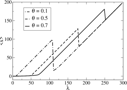
Figure 7: Role of the threshold $\theta$. Other computation parameters: $N=100$; $M=1$; $L=300$; $k_{\lambda}=100$; $A=5$; $K=0.1$; $\beta=2$.

As just discussed, the role of the folding prize and of the harmonic constant is related to the enthalpic term of the free energy. By contrast, the folding threshold $\theta$ influences the entropic contribution to the free energy. A small value of $\theta$ in fact, implies that only a small fraction of the contacts can be broken without loss of the folding prize. If $m<\theta N$ represents the number of broken contacts in a moment preceding the unfolding event, then the number of microscopic conformations allowed will be $g(n,N)=\binom{N}{n}$, and the entropy will be $S=-T\log[g(n,N)]$. If $\theta<0.5$, the unraveling of the domain will increase the degeneracy $g(n,N)$ and thus the entropy, so that a moderate extension of the spring will be sufficient for the enthalpic term to be more than compensated by the entropic one. By contrast, when $\theta\geq 0.5$, the breakdown of the domain and the resulting increase in the number of disrupted contacts, will bring the degeneracy and the entropy further away from the maximum thus disfavouring the unfolding event and causing the peak of the $(x,\lambda)$ profile to become higher. The pattern of increase in height of the unfolding peak as $\theta$ takes on higher values is shown in Figure 7.

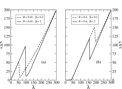
Figure 8: Interplay between the folding threshold $\theta$ and the inverse temperature $\beta$. For small $\theta$s (a) higher temperatures favour the unfolding, whereas the opposite is true for large $\theta$s (b). Common computation parameters: $N=100$; $M=1$; $L=300$; $k_{\lambda}=100$; $A=5$; K = 0.1.

The relevance of the entropic contribution on free energy computation strongly depends on temperature that may amplify the role of the threshold $\theta$. As already noticed, in fact, when $\theta<0.5$, the breakdown of the domain is entropically favoured as it brings the degeneracy closer to its maximum. Since this gain in entropy becomes larger and larger as the temperature is increased, for small $\theta$ the unfolding event becomes more and more favourable as $\beta$ is decreased, and the height of the peak of the $(x,\lambda)$ plot will also decrease accordingly. For $\theta\geq 0.5$ the opposite pattern can be observed. In fact, the entropy loss due to the decrease of the degeneracy resulting from the unfolding event, is magnified as $\beta$ is decreased leading to higher and higher peaks in the $(x,\lambda)$ plot. The interplay between the parameters $\theta$ and $\beta$ is shown in Figure 8.

III.3 Coupling and fluctuations

Figure 9: Role of fluctuations. Panels (a) and (b): a threshold lower than 0.5 ($\theta=0.1$) causes the first unfolding event to favour the following ones. Panels (c) and (d): the first unfolding event does not affect the second and third ones as a result of the high threshold $\theta=0.5$. Computation parameters: $N=100$; $M=3$; $L=400$; $k_{\lambda}=400$; $A=1$; $K=0.05$; $\beta=2$.

Figure 10: Free energy landscape under the action of an increasing elastic force in correspondence of the unfolding peak shown in the top left panel of Figure 9. Simulation parameters: $N=100$; $M=3$; $L=400$; $k_{\lambda}=400$; $A=1$; $\theta=0.1$; $K=0.05$; $\beta=2$.

Before studying the mutual influence of the unfolding events, let us illustrate the features of the free energy landscape of a single module near the unfolding transition. In Figure 10 we show the evolution of the free energy landscape in correspondence of the unfolding transition in a simulation with $M=3$ and $\theta=0.1$ (see also top left panel of Fig. 9). The profile is characterized by a cusp-like, narrow well corresponding to the folded state, and a wide, smooth well related to the unfolded state. The width of the two wells, in fact, depends on the number of conformations that the system can explore: in the folded state, the system is stretched due to the action of the spring and no fluctuations are allowed so that only one conformation will be populated; after the transition, the residues of the collapsed domain become free to fluctuate and many conformations will be explored thus determining a very wide well in the free energy profile. The Figure shows that for low values of $\lambda$ (and thus low values of the elastic force), the free energy of the reference folded state $G_{0}$ is lower than that of the unfolded state $G$, thus forbidding the breakdown of the domain; as $\lambda$ is increased, the free energy of the folded state increases, until it finally becomes higher than that of the folded conformation and the stretching transition occurs. This is a typical example of a first-order phase transition.

We now consider a polymer composed by $M=3$ tandem repeats with $N=100$ contacts each. In Figure 9 we compare two simulations performed with the same parameter set except for a different threshold $\theta$. In the simulation with $\theta=0.1$ the peaks corresponding to the second and third unfolding events are less pronounced than the first one thus suggesting that the unfolding of a domain actually favours further unfolding events. Conversely, in the simulation with $\theta=0.5$, the three peaks feature almost the same height showing that the first unfolding event has little or no influence at all on the following ones.

Each unfolding event in Figure 9 corresponds to a peak in the variance plot because the unraveling of a domain increases the fluctuations of the polymer and spring length. The variance peaks are characterized by a high and narrow spike followed by a smoother region that decreases more slowly. The shape of the variance peak is related to the regions of the free energy landscape explored by the system during the unfolding transition. The spikes in the variance plots (that are truncated for the sake of graphical clarity) correspond to the situation with $G=G_{0}$ when both wells are explored by the system and the variance $\sigma_{x}^{2}$ is related to the distance between the two wells. On the other hand, the smooth regions of the variance plots refer to the case with $G<G_{0}$ when the system only explores the unfolded region of the free energy landscape whose width correlates with the variance.

Figure 9 shows that the height of the smooth region of the variance peaks increases with the order of the unfolding event. This trend is due to the fact that, with each unfolding event, $N(1-\theta)$ new monomers become free to fluctuate and the number of accessible conformations increases accordingly. Figure 9 also shows that the value of the variance $\sigma_{x}^{2}$ after each unfolding event, gradually decrease as $\lambda$ is increased, because the disruption of the contacts of the domain just collapsed allow an extension of the molecule in the direction of the pulling force so as to avoid as far as possible a further stretching of the spring that would cause an increase in energy. As a result, narrower and narrower regions of the conformation space become accessible to the polymer and the variance is lowered. It is worthwhile noticing, however, that the extension of the unfolded domain is hindered by the subsequent decrease in entropy so that the number of contacts actually broken before each unfolding event is smaller than the maximum number allowed by the loss of the folding prize in the previous domain breakdown.

When $\theta=0.1$, 26 contacts (a number of the order of $\theta NM$) are broken before the first unfolding event. This value is consistent with the number of contacts that can be disrupted without loss of the folding prize. After the first collapse event, the number of contacts broken in the simulation rises to 115, thus determining an increase of the fluctuations and favouring the breakdown of another domain. This explains why the second peak of the $(x,\lambda)$ plot is less pronounced than the first one. The occurrence of the second unfolding determines a further increase of the number of cleaved contacts to 205. This results in a easy breakdown of the last domain of the protein and the last peak of the $(x,\lambda)$ plot is therefore less high than the second one.

This scenario is significantly different for $\theta=0.5$. For large values of $\theta$, in fact, only a small number of residues can be recruited for fluctuations after each unfolding event. As a consequence, the variance $\sigma_{x}^{2}$ rapidly goes to zero after each unfolding event and the fluctuations are extinguished before the force threshold for unfolding can be crossed. The following unfolding events, similarly to the first one, will occur when the increase in harmonic energy balances the loss of the folding prize and therefore the height of the unfolding $\langle x\rangle$-peaks will be roughly the same.

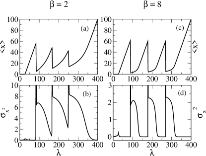
Figure 11: Effect of temperature on the relative heights of the peaks of the saw-tooth profile. For $\theta=0.1$, if the temperature is sufficiently high ($\beta=2$, panels (a) and (b)), the first unfolding event favours the following ones due to the role of fluctuations. At low temperatures however ($\beta=8$, panels (c) and (d) ), the fluctuations rapidly become negligible and the heights of the peaks become roughly the same due to the identical energetic features of the domains. Computation parameters: $N=100$; $M=3$; $L=400$; $k_{\lambda}=400$; $A=1$; $\theta=0.1$; $K=0.05$.

The role of fluctuations in determining the relative heights of the peaks of the $(x,\lambda)$ plot, and thus the coupling among domains, is confirmed through simulations performed at different temperatures. At very low temperatures, in fact, the entropic term of the free energy becomes negligible and the height of the peaks of the $(x,\lambda)$ plot only depends on the energetic term. As we are considering a protein composed by identical domains, we expect the $x(\lambda)$ peaks to be identical if the temperature is sufficiently low. This pattern can be observed in Figure 11 where we compare two simulations performed at different temperatures, namely $\beta=2$ and $\beta=8$.

III.4 Pulling rate effects

Figure 12: Monte Carlo computations of stretching and refolding: the non-superposability of the profiles is a signature of the irreversibility of the process. Simulation parameters: $N=100$; $M=3$; $L=450$; $k_{\lambda}=100$; $T=1000$; $A=1$; $\theta=0.3$; $K=0.5$; $\beta=2$.

Up to now, we discussed equilibrium stretching computations, i.e. we assumed an infinitely slow pulling. However, at the typical time scales of an AFM stretching experiment, the polymer is pulled at a finite velocity and the unfolding is a non-equilibrium process, as testified by the differences between the unfolding and the refolding force-extension profiles (see e.g. Figure 12). In fact, while the unfolding profile features the typical saw-tooth pattern, upon relaxation of the unfolded polymer, the trace exhibits no discontinuities that would indicate refolding.

A consequence of the irreversibility of the stretching process is that the unfolding force depends on the pulling speed. Actually, if the loading rate $r_{f}=k_{f}v$ (with $k_{f}$ being the elastic constant and $v$ the pulling velocity) is sufficiently small, thermal fluctuations are allowed enough time to overcome the energy barrier and the unfolding force will be low.

Several experimental works Ig ; Carrion-veloc ; Fritz-veloc ; Merkel-veloc reported a logarithmic dependence of the unfolding force on the loading rate in the case where a single energy barrier is present along the reaction path. The analytic expression of the relation between force and loading rate was derived Bell ; Evans-veloc ; Tavan-veloc within the frame of Kramer’s theory for a simple two-state model, by assuming that the external force reduces the height of the energy barrier,

$$\langle F_{max}\rangle=\frac{k_{B}T}{\Delta x}\log\left(\frac{Kv\Delta x}{k_{0}k_{B}T}\right),$$ (4)

where $k_{B}$ is Boltzmann constant, $T$ is the absolute temperature, $\Delta x$ is the distance between the minimum corresponding to the folded state and the activation barrier of the energy landscape, $v$ is the pulling speed, $K$ is the cantilever harmonic constant and $k_{0}$ is the spontaneous unfolding rate.

Recently Schlierf , it has been shown that the probability distribution of the force at various pulling rates does not follow the simple Bell law, requiring the full Kramer’s theory and predicting small corrections to the logaritmic behavior of the most probable force.

Figure 13: Comparison between the equilibrium computations and a set of Monte Carlo simulations with different numbers of MC steps. The peaks of the $(x-\lambda)$ profile become lower and lower and the MC simulations converge to the equilibrium scenario as the number of MC steps is increased. Simulation parameters: $N=10$; $M=3$; $L=70$; $k_{\lambda}=100$; $A=1$; $\theta=0.2$; $K=0.1$; $\beta=2$. Notice that, using a smaller value of $N$, the equilibrium profile is smoother than that in Figure 9, Figure 11 and preceding ones.

We limit here to a preliminary illustration of a series of Monte Carlo simulations with different number of steps $T$ considering the pulling speed as being proportional to $1/T$. A more detailed analysis will be presented in a forthcoming paper.

Figure 13 shows that, as the number of Monte-Carlo (MC) steps is increased, the $(x-\lambda)$ plot becomes closer and closer to the profile yielded by the equilibrium simulation. In particular, a small number of MC steps, i.e. a fast pulling, corresponds to high peaks of the $(x-\lambda)$ profile, whereas larger numbers of steps correspond to less and less pronounced peaks and thus, smaller unfolding forces.

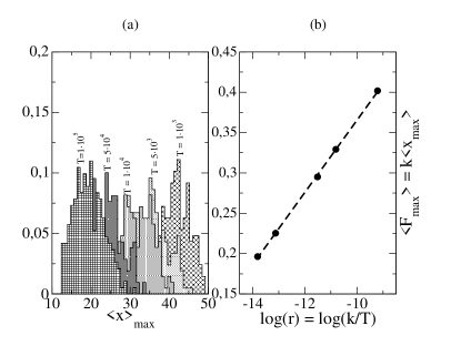
Figure 14: Statistical analysis of unfolding forces in 5 sets of 100 independent Monte Carlo runs with different numbers of MC steps. Panel (a): histograms of spring extensions at the rupture point; panel (b): linear fit of the average rupture force as a function of the logarithm of the loading rate. Simulation parameters: $N=10$; $M=3$; $L=70$; $k_{\lambda}=100$; $A=10$; $\theta=0.2$; $K=0.1$; $\beta=2$.

We performed a series of 100 independent MC runs for 5 different values of $T$: $1\cdot 10^{3}$, $5\cdot 10^{3}$, $1\cdot 10^{4}$, $5\cdot 10^{4}$ and $1\cdot 10^{5}$. For each series of runs we built the histograms of the rupture spring elongations and we plotted the mean value of the histogram as a function of the logarithm of the loading rate. Finally, the set of points thus obtained was linearly fitted. As shown in Figure 14, the histograms, shift to lower values as the number of MC steps increases. Figure 14 also shows that the mean rupture forces computed from the histograms, feature an excellent linear correlation with the logarithm of the loading rate (correlation coefficient $r_{c}=0.99$).

If Eq. 4 is explicitly rearranged so as to show the linear dependence of $\langle F_{max}\rangle$ on $\log(Kv)$, the coefficients of the linear equation can be equated to the corresponding parameters $\gamma_{1}$ and $\gamma_{2}$ of the regression line $\langle F_{max}\rangle=\gamma_{1}\log(Kv)+\gamma_{2}$, so as to build the following system of equations:

$$\left\{\begin{array}[]{lll}\frac{k_{B}T}{\Delta x}&=&\gamma_{1}\\ \frac{k_{B}T}{\Delta x}\log\left(\frac{\Delta x}{k_{0}k_{B}T}\right)&=&\gamma_{2}\end{array}\right.$$

From the first equation of the system it is possible to compute the width of the activation barrier $\Delta x=11.17$; this value can then be substituted into the second equation so as to determine $k_{0}=2.93\cdot 10^{-7}$. The spontaneous unfolding rate $k_{0}$, on turn, is related to the height of the activation barrier for the unfolding process,

$$k_{0}=\omega e^{-\Delta G_{u}^{\dagger}/k_{B}T},$$

where $\omega$, as explained by Kramer’s theory, is the reciprocal of a diffusive relaxation time. This simple computation shows how stretching experiments and simulations provide easy access to important features of the free energy landscape. In a forthcoming paper we aim at investigating the relations relating the barrier width $\Delta x$ and the spontaneous unfolding rate $k_{0}$ with molecular properties such as the folding prize $A$, the threshold $\theta$, the number $N$ and the length $M$ of the domains.

III.5 High pulling rate limit

Let us investigate the dependence of the Monte Carlo simulations on the number of Monte-Carlo steps $T$, that we can interpret as a measure of the pulling speed. In fact, in the limit of an extremely high pulling speed, we can assume that for each value of $\lambda$ the polymer can adopt just a single (or at most, a few) conformation, so that the entropic contribution can be neglected in the computations.

The mechanism outlined in Section III.2 shows that the key event is the loss of the folding prize determining the complete extension of the protein domain and the subsequent relaxation of the spring. The problem thus arises to identify the factors affecting the probability of this crucial step. More specifically, suppose in a domain a number of contacts just below the threshold to keep the folding prize has been broken. What is the probability $\pi$ that one more contact will be cleaved within the next $\nu$ steps ?

In order to answer this question, it is necessary to compute the energy difference associated with the transition. Let $x$ be the length of the spring when a number of contacts just below the threshold $\theta N$ has been disrupted: the system retains the prize $A$. If one more contact is broken, the prize is lost and the spring will be correspondingly shortened. In particular, by assuming each contact breakdown to cause a unit increase in length of the polymer, the new length of the spring will be $x-1$. The energy difference between the two states can thus be computed as

$$\Delta E=\left(\frac{1}{2}Kx^{2}-A\right)-\frac{1}{2}K(x-1)^{2}\cong Kx-A,$$

where a term $K/2$ has been neglected. We can now compute the probability to destroy a contact in a single step

$$p=\frac{1}{1+e^{-\beta\Delta E}}=\frac{1}{1+e^{\beta(A=Kx)}}.$$

Finally, the probability to break a contact in $\nu$ steps is given by the sum of a geometric progression

$$\pi=\sum_{i=0}^{\nu}(1=p)^{i}p=1-(1-p)^{\nu}.$$

The computations thus show that the domain unfolds with a probability depending on the prize, the cantilever stiffness, the temperature and the pulling velocity (that in our simulations is related to the number $T$ of Monte Carlo steps).

Figure 15: Effect of the simulation parameters on the height of the unfolding ramp. Unless otherwise indicated in the legend, the simulation parameters are: $N=100$; $M=1$; $L=150$; $k_{\lambda}=50$; $T=100$; $A=0.1$; $\theta=0.2$; $K=0.1$; $\beta=2$.

In order to test our analytical treatment of the unfolding probability, we performed a series of MC simulations differing from a reference one just for a parameter (Figure 15). The key parameters characterizing the reference simulations are: $T=100$, $A=0.1$, $K=0.1$, $\beta=2$. In agreement with the analytic computation, the simulations show that an increase in the number of Monte Carlo steps ($T=10^{4}$), an increase in temperature ($\beta=1.5$), a decrease of the folding prize ($A=8.5\times 10^{-2}$), and an increase of the spring constant ($K=1.25\times 10^{-1}$), all result in an increase of the unfolding probability, thus reducing the height of the peak in the $(x-\lambda)$-plot.

IV Conclusions

We developed an extremely simplified model of polymer stretching in which the molecule is portrayed as a series of modules, represented as an array of contacts,and a harmonic spring (the cantilever). The chemical interactions stabilizing the native conformation are simply modeled as a folding prize gained by domains where the fraction of folded monomers is above a pre-chosen threshold. Our model is consistent with recent findings in Refs Schulten1 ; Schulten2 ; Schulten3 , showing that the unraveling of the titin Immunoglobulin domain occurs very rapidly only after the breakdown of a critical number of key hydrogen-bonds. The attribution of a folding prize when a threshold value of the fraction of native contacts is crossed, also makes our approach equivalent to a Gō-model with force rescaling Chan . However, our model is thus significantly simpler than other models commonly used to study mechanical unfolding such as the WLC and FJC models and the detailed all-atom, topological and united-residue models employed for steered molecular dynamics simulations. Yet, our model is detailed enough to reproduce many qualitative features of the force-extension profiles recorded in AFM experiments. In particular, our model correctly reproduces the typical saw-tooth pattern with peaks characterized by a height dependent on the folding prize, the temperature and the pulling velocity.

In our study, a particular attention was paid to the relation between the heights of successive peaks in the force-extension plot. This point is quite intriguing as experimental data show that the force of unfolding tends to increase with each unfolding event, suggesting that the protein domains unfold following an increasing order of mechanical stability Li2000 . A possible explanation suggested by the literature is that the domains of the engineered modular constructs used in AFM experiments are not identical but just structurally similar Rief . This argument may be correct in the case of real proteins where the differences in mechanical stability of the tandem repeats of the construct may arise from their different position in the tridimensional structure of the molecule. In a computer simulation, however, the domains are all perfectly identical and the explanation for the staircase pattern of unfolding peaks must be sought elsewhere. This behavior has been ascribed to an independent breaking probability of each domain. This hypothesis is however not consistent with the fact that the cantilever couples the fluctuations of all domains. Our unified treatment allows to keep into consideration all contributions, and to obtain the correct equilibrium curves, that generally do not exhibit this effect. However, a detailed study of out-of-equilibrium extension curves, shows that this behavior is consistent with a finite pulling speed, i.e. it can be ascribed to a dynamical source.

Our results appear to be in agreement with recent findings by Cieplak Cieplak in steered molecular dynamics simulations of titin and calmodulin unfolding using a Go-like model. In particular,it was found that an increase in thermal fluctuations results in a lowering of the force peaks and in their earlier occurrence during stretching.

An interesting feature of AFM stretching experiments is that the mean unfolding force is a logarithmic function of the pulling rate. This pattern reflects the role of thermal fluctuations: if the pulling speed is sufficiently low, then there will be enough time for thermal fluctuations to drive the polymer over the free energy barrier and the unfolding force will be accordingly low. The ability to reproduce this pattern constitutes a benchmark for any stretching model. In order to test our model, we performed a series of Monte Carlo simulations with different numbers $T$ of MC-steps and regarding the pulling velocity to be proportional to $1/T$. Our toy-model, despite its extreme simplicity, correctly reproduced the linear dependence of the mean unfolding force on the logarithm of the pulling rate.

In summary, our simple model including harmonic and long-range energy contributions, is not only capable of reproducing the force-extension saw-tooth pattern, but it also yields force spectra displaying the correct logarithmic dependence of $\langle F_{max}\rangle$ on $Kv$ reported in experimental works. Finally, our model provides a simple explanation of the influence of each unfolding event on the following ones, based on the role of fluctuations. Our work thus shows how minimal models can be valuable tools even in the study of complex molecular systems.

References

- (1) M.S.Z. Kellermayer, Physiol. Meas. 26, R119 (2005).
- (2) E.J. Peterman, H. Sosa and W.E. Moerner, Ann. Rev. Phys. Chem. 55, 79 (2004).
- (3) R.B. Best, D.J. Brockwell, J.L. Toca-Herrera, A.W. Blake, D.A. Smith, S.E Radford and J. Clarke, Anal. Chim. Acta 479, 87 (2003).
- (4) X. Michalet and S. Weiss, C. R. Physique 3, 619 (2002).
- (5) D.J.Muller, H. Janovjak, T. Lehto, L. Kuerschner and K.Anderson, Prog. Biophys. Mol. Biol. 79, 1 (2002).
- (6) T.E. Fisher, P.E. Marszalek and J.M. Fernandez, Nature Struct. Biol. 7, 719 (2000).
- (7) T.E.Fisher, M.Carrion-Vazquez, A.F. Oberhauser, H. Li, P.E. Marszalek and J.M. Fernandez, Neuron 27, 435 (2000).
- (8) D. Keller, D. Swigon and C. Bustamante, Biophys. J. 84, 733 (2003).
- (9) M.Rief, M. Gautel, F. Oesterhelt, J.M. Fernandez and H.E. Gaub, Science 276, 1109 (1997).
- (10) A.F.Oberhauser, P.E. Marszalek, H.P. Erickson and J.M. Fernandez, Nature 393, 181 (1998).
- (11) M.Carrion-Vazquez, A.F. Oberhauser, T.E. Fisher, P.E. Marszalek, H. Li and J.M. Fernandez, Prog. Biophys. Mol. Biol. 74, 63 (2000).
- (12) M.Rief, J. Pascual, M. Saraste and H.E. Gaub, J. Mol. Biol. 286, 553 (1999).
- (13) C. Bustamante, J.F. Marko, E.D. Siggia and S. Smith, Science 265, 1599 (1994).
- (14) S.B.Smith, L. Finzi and C. Bustamante, Science 258, 1122 (1992).
- (15) M. Rief, J.M. Fernandez and H.E. Gaub, Phys. Rev. Lett. 81, 4764 (1998).
- (16) E. Evans and K. Ritchie, Biophys. J. 72, 1541 (1997).
- (17) E. Evans, D. Berk and A. Leung, Biophys J. 59, 838 (1991).
- (18) G.I. Bell, Science 200, 618 (1978).
- (19) M. Sclierf and M. Rief, Biophys. J. 90 L33 (2006).
- (20) M. Zemanová and T. Bleha, Macromol. Theory Simul. 14, 596 (2005).
- (21) P.E. Marszalek, H. Lu, H. Li, Carrion-Vazquez, A.M. Oberhauser, K. Schulten and J.M. Fernandez, Nature 402, 100 (1999).
- (22) H. Lu, A. Isralewitz, A. Krammer, V. Vogel and K. Schulten, Biophys. J. 75, 662 (1998).
- (23) H. Lu and K. Sculten, Chem. Phys. 247, 141 (1999).
- (24) D.E. Makarov, P.K. Hansma and H. Metiu, J. Chem. Phys. 114, 9663 (2001).
- (25) M. Rief and H. Grubmüller, Chem. Phys. Chem. 3, 255 (2002).
- (26) H. Kaya, Z. Liu and H.S. Chan, Biophys. J. 89, 520 (2005).
- (27) F. Cecconi, C. Guardiani and R. Livi Biophys. J. 91 694 (2006).
- (28) O.V. Galzitskaya and A.V. Finkelstein, Proc. Natl. Acad. Sci. USA 96, 11299 (1999).
- (29) B.H. Zimm and J.K. Bragg, J. Chem. Phys. 31, 526 (1959).
- (30) M. Carrion-Vazquez, A.F. Oberhauser, S.B. Fowler, P.E. Marszalek, S.E. Broedel, J.Clarke and J.M. Fernandez, Proc. Natl. Acad. Sci. USA 96, 3694 (1999).
- (31) J. Fritz, A.G. Katopodis, F. Kolbinger and D. Anselmetti, Proc. Natl. Acad. Sci. USA 95, 12283 (1998).
- (32) R. Merkel, P. Nassoy, A. Leung, K. Ritchie, and E. Evans, Nature 397, 50 (1999).
- (33) E. Evans, Ann. Rev. Biophys. Biomol. Struct. 30, 105 (2001).
- (34) H. Grubmüller, B. Heymann and P. Tavan, Science 271, 997 (1996).
- (35) H. Li, A.F. Oberhauser, S.B. Fowler, J. Clarke and J.M. Fernandez, Proc. Natl. Acad. Sci. USA 97, 6527 (2000).
- (36) M. Cieplak, Physica A 352, 28 (2005).
- (37) Forman J.R., Qamar S., Paci E., Sandford R.N., Clarke J. (2005), The remarkable mechanical strength of polycystin-1 supports a direct role in mechanotransduction, J. Mol. Biol., 349, 861-871.
- (38) Kirmizialtin S., Huang L. and Makarov D.E. (2005), Topography of the free-energy landscape probed via mechanical unfolding of proteins, J. Chem. Phys., 122, 234915.
- (39) Gräter F., Shen J., Jiang H., Gautel M. and Grubmüller H. (2005), Mechanically induced titin kinase activation studied by force-probe molecular dynamics simulations, Biophys. J., 88, 790-804.
- (40) Ng S.P., Rounsevell R.W.S., Steward A., Geierhaas C.D., Williams P.M., Paci E. and Clarke J. (2005), Mechanical unfolding of TNfn3: the unfolding pathway of a fnIII domain probed by protein engineering, AFM and MD simulation, J. Mol. Biol., 350, 776-789.
- (41) Clementi C., Nymeyer H. and Onuchic J.N. (2000), Topological and energetic factors: what determines the structural details of the transition state ensemble and ”en-route” intermediates for protein folding ? An investigation for small globular proteins J. Mol. Biol., 298, 937-953.