Epidemic outbreaks on structured populations

Alexei Vazquez
The Simons Center for Systems Biology
Institute for Advanced Study, Einstein Dr, Princeton, NJ 08540, USA
Abstract

Our chances to halt epidemic outbreaks rely on how accurately we represent the population structure underlying the disease spread. When analyzing global epidemics this force us to consider metapopulation models taking into account intra- and inter-community interactions. Recently Watts et al introduced a metapopulation model which accounts for several features observed in real outbreaks [Watts et al, PNAS 102, 11157 (2005)]. In this work I provide an analytical solution to this model, enhancing our understanding of the model and the epidemic outbreaks it represents. First, I demonstrate that depending on the intra-community expected outbreak size and the fraction of social bridges the epidemic outbreaks die out or there is a finite probability to observe a global epidemics. Second, I show that the global scenario is characterized by resurgent epidemics, their number increasing with increasing the intra-community average distance between individuals. Finally, I present empirical data for the AIDS epidemics supporting the model predictions.

Human populations are structured in communities representing geographical locations and other factors leading to partial segregation. This population structure has a strong impact on the spreading patterns of infectious diseases among humans, forcing us to consider metapopulation models making an explicit distinction between the intra- inter-community interactions [Rvachev & Longini, 1985, Sattenspiel & Dietz, 1995]. The increase in model realism is paid, however, by an increase in model complexity. Detailed metapopulation models are difficult to build and as a consequence they are available for a few locations in the world [Rvachev & Longini, 1985, Flahault et al., 1988, Eubank et al., 2004, Germann et al., 2006] or they cover a single route of global transmission [Hufnagel et al., 2004, Colizza et al., 2006].

Recently Watts et al [Watts et al., 2005] introduced a simple metapopulation model making an explicit distinction between the intra- and inter-community interactions. In spite of the model simplicity it accounts for several features observed in real epidemic outbreaks. In particular, the numerical results indicate the existence of a transition from local to global epidemics when the expected number of infected individuals changing community reaches one [Watts et al., 2005]. I go a step forward and provide an analytical solution to the Watts et al metapopulation model. I demonstrate that there is indeed a phase transition when the expected number of infected individuals changing community reaches one. This analytical solution allow us to obtain a much deeper insight into the main features of global epidemic outbreaks.

\ellipse29962996\path(835,9012)(1435,8712) \path(1193.505,8765.666)(1435.000,8712.000)(1247.170,8872.997) \path(1435,8712)(2035,8412) \path(1793.505,8465.666)(2035.000,8412.000)(1847.170,8572.997) \path(1435,8712)(2035,9012) \path(1847.170,8851.003)(2035.000,9012.000)(1793.505,8958.334) \path(835,9012)(1435,9312) \path(1247.170,9151.003)(1435.000,9312.000)(1193.505,9258.334) \path(2035,9012)(2635,9012) \path(2395.000,8952.000)(2635.000,9012.000)(2395.000,9072.000) \path(2035,9012)(2635,8712) \path(2393.505,8765.666)(2635.000,8712.000)(2447.170,8872.997) \path(2635,9012)(3235,9012) \path(2995.000,8952.000)(3235.000,9012.000)(2995.000,9072.000) \path(1435,9312)(2035,9312) \path(1795.000,9252.000)(2035.000,9312.000)(1795.000,9372.000) \path(2035,9312)(2635,9312) \path(2395.000,9252.000)(2635.000,9312.000)(2395.000,9372.000) \path(2035,9312)(2635,9612) \path(2447.170,9451.003)(2635.000,9612.000)(2393.505,9558.334) \path(2635,9312)(3235,9312) \path(2995.000,9252.000)(3235.000,9312.000)(2995.000,9372.000) \path(1435,9312)(2035,9612) \path(1847.170,9451.003)(2035.000,9612.000)(1793.505,9558.334) \path(2635,8712)(3235,8712) \path(2995.000,8652.000)(3235.000,8712.000)(2995.000,8772.000) \path(2635,8712)(3235,8412) \path(2993.505,8465.666)(3235.000,8412.000)(3047.170,8572.997) \dashline120.000(3235,9012)(4435,9012) \blacken\path(4075.000,8922.000)(4435.000,9012.000)(4075.000,9102.000)(4183.000,9012.000)(4075.000,8922.000) \dashline120.000(2035,8412)(235,5712) \blacken\path(359.808,6061.461)(235.000,5712.000)(509.577,5961.615)(374.784,5921.677)(359.808,6061.461) \dashline120.000(2635,5712)(3835,5412) \blacken\path(3463.920,5412.000)(3835.000,5412.000)(3507.577,5586.626)(3590.524,5473.119)(3463.920,5412.000) \dashline120.000(2035,4812)(535,2262) \blacken\path(639.953,2617.928)(535.000,2262.000)(795.101,2526.665)(662.769,2479.207)(639.953,2617.928) \dashline120.000(5635,4812)(7435,2712) \blacken\path(7132.382,2926.761)(7435.000,2712.000)(7269.048,3043.904)(7271.001,2903.333)(7132.382,2926.761) \path(235,5712)(835,5412) \path(593.505,5465.666)(835.000,5412.000)(647.170,5572.997) \path(835,5412)(1435,5112) \path(1193.505,5165.666)(1435.000,5112.000)(1247.170,5272.997) \path(835,5412)(1435,5712) \path(1247.170,5551.003)(1435.000,5712.000)(1193.505,5658.334) \path(235,5712)(835,6012) \path(647.170,5851.003)(835.000,6012.000)(593.505,5958.334) \path(1435,5712)(2035,5712) \path(1795.000,5652.000)(2035.000,5712.000)(1795.000,5772.000) \path(1435,5712)(2035,5412) \path(1793.505,5465.666)(2035.000,5412.000)(1847.170,5572.997) \path(2035,5712)(2635,5712) \path(2395.000,5652.000)(2635.000,5712.000)(2395.000,5772.000) \path(835,6012)(1435,6012) \path(1195.000,5952.000)(1435.000,6012.000)(1195.000,6072.000) \path(1435,6012)(2035,6012) \path(1795.000,5952.000)(2035.000,6012.000)(1795.000,6072.000) \path(1435,6012)(2035,6312) \path(1847.170,6151.003)(2035.000,6312.000)(1793.505,6258.334) \path(2035,6012)(2635,6012) \path(2395.000,5952.000)(2635.000,6012.000)(2395.000,6072.000) \path(835,6012)(1435,6312) \path(1247.170,6151.003)(1435.000,6312.000)(1193.505,6258.334) \path(2035,5412)(2635,5412) \path(2395.000,5352.000)(2635.000,5412.000)(2395.000,5472.000) \path(2035,5412)(2635,5112) \path(2393.505,5165.666)(2635.000,5112.000)(2447.170,5272.997) \path(1435,5112)(2035,5112) \path(1795.000,5052.000)(2035.000,5112.000)(1795.000,5172.000) \path(1435,5112)(2035,4812) \path(1793.505,4865.666)(2035.000,4812.000)(1847.170,4972.997) \path(535,2262)(1135,1962) \path(893.505,2015.666)(1135.000,1962.000)(947.170,2122.997) \path(1135,1962)(1735,1662) \path(1493.505,1715.666)(1735.000,1662.000)(1547.170,1822.997) \path(1135,1962)(1735,2262) \path(1547.170,2101.003)(1735.000,2262.000)(1493.505,2208.334) \path(535,2262)(1135,2562) \path(947.170,2401.003)(1135.000,2562.000)(893.505,2508.334) \path(1735,2262)(2335,2262) \path(2095.000,2202.000)(2335.000,2262.000)(2095.000,2322.000) \path(1135,2562)(1735,2562) \path(1495.000,2502.000)(1735.000,2562.000)(1495.000,2622.000) \path(1735,2562)(2335,2562) \path(2095.000,2502.000)(2335.000,2562.000)(2095.000,2622.000) \path(1735,2562)(2335,2862) \path(2147.170,2701.003)(2335.000,2862.000)(2093.505,2808.334) \path(2335,2562)(2935,2562) \path(2695.000,2502.000)(2935.000,2562.000)(2695.000,2622.000) \path(1135,2562)(1735,2862) \path(1547.170,2701.003)(1735.000,2862.000)(1493.505,2808.334) \path(1735,1662)(2335,1662) \path(2095.000,1602.000)(2335.000,1662.000)(2095.000,1722.000) \path(1735,1662)(2335,1362) \path(2093.505,1415.666)(2335.000,1362.000)(2147.170,1522.997) \path(3835,5412)(4435,5112) \path(4193.505,5165.666)(4435.000,5112.000)(4247.170,5272.997) \path(4435,5112)(5035,4812) \path(4793.505,4865.666)(5035.000,4812.000)(4847.170,4972.997) \path(3835,5412)(4435,5712) \path(4247.170,5551.003)(4435.000,5712.000)(4193.505,5658.334) \path(5635,5412)(6235,5412) \path(5995.000,5352.000)(6235.000,5412.000)(5995.000,5472.000) \path(4435,5712)(5035,5712) \path(4795.000,5652.000)(5035.000,5712.000)(4795.000,5772.000) \path(5035,5712)(5635,5712) \path(5395.000,5652.000)(5635.000,5712.000)(5395.000,5772.000) \path(5035,5712)(5635,6012) \path(5447.170,5851.003)(5635.000,6012.000)(5393.505,5958.334) \path(5635,5712)(6235,5712) \path(5995.000,5652.000)(6235.000,5712.000)(5995.000,5772.000) \path(4435,5712)(5035,6012) \path(4847.170,5851.003)(5035.000,6012.000)(4793.505,5958.334) \path(5635,5112)(6235,5112) \path(5995.000,5052.000)(6235.000,5112.000)(5995.000,5172.000) \path(5635,5112)(6235,4812) \path(5993.505,4865.666)(6235.000,4812.000)(6047.170,4972.997) \path(5035,4812)(5635,4812) \path(5395.000,4752.000)(5635.000,4812.000)(5395.000,4872.000) \path(5035,4812)(5635,4512) \path(5393.505,4565.666)(5635.000,4512.000)(5447.170,4672.997) \path(4435,9012)(5035,8712) \path(4793.505,8765.666)(5035.000,8712.000)(4847.170,8872.997) \path(5035,8712)(5635,8412) \path(5393.505,8465.666)(5635.000,8412.000)(5447.170,8572.997) \path(5035,8712)(5635,9012) \path(5447.170,8851.003)(5635.000,9012.000)(5393.505,8958.334) \path(4435,9012)(5035,9312) \path(4847.170,9151.003)(5035.000,9312.000)(4793.505,9258.334) \path(5635,9012)(6235,9012) \path(5995.000,8952.000)(6235.000,9012.000)(5995.000,9072.000) \path(6235,9012)(6835,9012) \path(6595.000,8952.000)(6835.000,9012.000)(6595.000,9072.000) \path(5035,9312)(5635,9312) \path(5395.000,9252.000)(5635.000,9312.000)(5395.000,9372.000) \path(5635,9312)(6235,9312) \path(5995.000,9252.000)(6235.000,9312.000)(5995.000,9372.000) \path(5635,9312)(6235,9612) \path(6047.170,9451.003)(6235.000,9612.000)(5993.505,9558.334) \path(6235,9312)(6835,9312) \path(6595.000,9252.000)(6835.000,9312.000)(6595.000,9372.000) \path(5035,9312)(5635,9612) \path(5447.170,9451.003)(5635.000,9612.000)(5393.505,9558.334) \path(5635,8412)(6235,8412) \path(5995.000,8352.000)(6235.000,8412.000)(5995.000,8472.000) \path(5635,8412)(6235,8112) \path(5993.505,8165.666)(6235.000,8112.000)(6047.170,8272.997) \path(7435,2712)(8035,2412) \path(7793.505,2465.666)(8035.000,2412.000)(7847.170,2572.997) \path(8035,2412)(8635,2112) \path(8393.505,2165.666)(8635.000,2112.000)(8447.170,2272.997) \path(7435,2712)(8035,3012) \path(7847.170,2851.003)(8035.000,3012.000)(7793.505,2958.334) \path(8035,3012)(8635,3012) \path(8395.000,2952.000)(8635.000,3012.000)(8395.000,3072.000) \path(8635,3012)(9235,3012) \path(8995.000,2952.000)(9235.000,3012.000)(8995.000,3072.000) \path(8635,3012)(9235,3312) \path(9047.170,3151.003)(9235.000,3312.000)(8993.505,3258.334) \path(9235,3012)(9835,3012) \path(9595.000,2952.000)(9835.000,3012.000)(9595.000,3072.000) \path(8035,3012)(8635,3312) \path(8447.170,3151.003)(8635.000,3312.000)(8393.505,3258.334) \path(8635,2112)(9235,2112) \path(8995.000,2052.000)(9235.000,2112.000)(8995.000,2172.000) \path(8635,2112)(9235,1812) \path(8993.505,1865.666)(9235.000,1812.000)(9047.170,1972.997) \path(5035,4812)(5635,5112) \path(5447.170,4951.003)(5635.000,5112.000)(5393.505,5058.334) \path(5035,4812)(5635,5412) \path(5507.721,5199.868)(5635.000,5412.000)(5422.868,5284.721) \ellipse29962996\ellipse29962996\ellipse29962996\ellipse29962996\ellipse29962996\ellipse29962996\ellipse29962996\whiten\ellipse212212\ellipse212212\blacken\ellipse212212\ellipse212212\blacken\ellipse212212\ellipse212212\whiten\ellipse212212\ellipse212212\whiten\ellipse212212\ellipse212212\whiten\ellipse212212\ellipse212212\whiten\ellipse212212\ellipse212212\whiten\ellipse212212\ellipse212212\whiten\ellipse212212\ellipse212212\whiten\ellipse212212\ellipse212212\whiten\ellipse212212\ellipse212212\whiten\ellipse212212\ellipse212212\whiten\ellipse212212\ellipse212212\whiten\ellipse212212\ellipse212212\whiten\ellipse212212\ellipse212212\whiten\ellipse212212\ellipse212212\whiten\ellipse212212\ellipse212212\blacken\ellipse212212\ellipse212212\whiten\ellipse212212\ellipse212212\whiten\ellipse212212\ellipse212212\whiten\ellipse212212\ellipse212212\whiten\ellipse212212\ellipse212212\whiten\ellipse212212\ellipse212212\whiten\ellipse212212\ellipse212212\whiten\ellipse212212\ellipse212212\whiten\ellipse212212\ellipse212212\whiten\ellipse212212\ellipse212212\blacken\ellipse212212\ellipse212212\whiten\ellipse212212\ellipse212212\whiten\ellipse212212\ellipse212212\whiten\ellipse212212\ellipse212212\whiten\ellipse212212\ellipse212212\whiten\ellipse212212\ellipse212212\whiten\ellipse212212\ellipse212212\whiten\ellipse212212\ellipse212212\whiten\ellipse212212\ellipse212212\whiten\ellipse212212\ellipse212212\whiten\ellipse212212\ellipse212212\whiten\ellipse212212\ellipse212212\whiten\ellipse212212\ellipse212212\whiten\ellipse212212\ellipse212212\whiten\ellipse212212\ellipse212212\whiten\ellipse212212\ellipse212212\whiten\ellipse212212\ellipse212212\whiten\ellipse212212\ellipse212212\whiten\ellipse212212\ellipse212212\whiten\ellipse212212\ellipse212212\blacken\ellipse212212\ellipse212212\whiten\ellipse212212\ellipse212212\whiten\ellipse212212\ellipse212212\whiten\ellipse212212\ellipse212212\whiten\ellipse212212\ellipse212212\whiten\ellipse212212\ellipse212212\whiten\ellipse212212\ellipse212212\whiten\ellipse212212\ellipse212212\whiten\ellipse212212\ellipse212212\blacken\ellipse212212\ellipse212212\whiten\ellipse212212\ellipse212212\whiten\ellipse212212\ellipse212212\whiten\ellipse212212\ellipse212212\whiten\ellipse212212\ellipse212212\whiten\ellipse212212\ellipse212212\whiten\ellipse212212\ellipse212212\blacken\ellipse212212\ellipse212212\whiten\ellipse212212\ellipse212212\whiten\ellipse212212\ellipse212212\whiten\ellipse212212\ellipse212212\whiten\ellipse212212\ellipse212212\whiten\ellipse212212\ellipse212212\whiten\ellipse212212\ellipse212212\whiten\ellipse212212\ellipse212212\whiten\ellipse212212\ellipse212212\whiten\ellipse212212\ellipse212212\whiten\ellipse212212\ellipse212212\whiten\ellipse212212\ellipse212212\whiten\ellipse212212\ellipse212212\whiten\ellipse212212\ellipse212212\blacken\ellipse212212\ellipse212212\whiten\ellipse212212\ellipse212212\whiten\ellipse212212\ellipse212212\whiten\ellipse212212\ellipse212212\whiten\ellipse212212\ellipse212212\whiten\ellipse212212\ellipse212212\whiten\ellipse212212\ellipse212212\whiten\ellipse212212\ellipse212212\whiten\ellipse212212\ellipse212212
Figure 1: Epidemic outbreak on a structured population: Schematic representation of a population structured in communities (big circles) and and the spread of an infectious disease inside and between communities. The individuals inside a community are divided between locals (open circles) and bridges (filled circles). The locals transmit the disease to other individuals inside the community (solid arcs) while the bridges transmit the disease to individuals in other communities (dashed arcs). For simplicity individuals that are not affected by the outbreak are not shown.

Model

Figure 1 illustrates the general features of an epidemic outbreak on a population structured in different communities. Starting from an index case a disease spreads widely inside a community thanks to the frequent intra-community interactions. In addition the disease is transmitted to other communities via individuals belonging to different communities. While the inter-community interactions may be rare they are determinant to understand the overall outbreak progression. Based on this picture I divide the population in two types or classes. The locals belonging to a single community and the social bridges belonging to different communities. In a first approximation I assume that (i) all communities are statistically equivalent, (ii) the mixing between the local and bridges is homogeneous, and (iii) social bridges belong to two populations. While these assumptions are off course approximations they allow us to gain insight into the problem. They could be relaxed in future works to include other factors such as degree correlations among interacting individuals [Vazquez, 2006c] and more realistic mixing patterns [Vazquez, 2006d].

An epidemic outbreak taking place inside a community is then modeled by a a multi-type branching process [Mode, 1971] starting from an index case (see Fig. 1). The key intra-community magnitudes are the reproductive number and the generation times [Anderson & May, 1991, Vazquez, 2006b]. The reproductive number is the average number of secondary cases generated by a primary case. The disease transmission introduces some biases towards individuals that interact more often. Therefore, I make an explicit distinction between the index case and other primary cases and denote their expected reproductive numbers by $R$ and $\tilde{R}$, respectively. The generation time $\tau$ is the time elapse from the infection of a primary case and the infection of a secondary case. It is a random variable characterized by the generation time distribution function $G(\tau)$. These magnitudes can be calculated for different models such as the susceptible infected recovered (SIR) model and they can be estimated from empirical data as well. Finally, a community outbreak is represented by a causal true rooted at the index case [Vazquez, 2006a, Vazquez, 2006b]. In this tree the generation of an infected case is given by the distance to the index case. Furthermore, the tree can have at most $D$ generations, where $D$ is the average distance between individuals inside a community.

\path(750,2058)(4050,2058) \path(3690.000,1968.000)(4050.000,2058.000)(3690.000,2148.000) \path(750,2058)(4050,258) \path(3690.861,351.376)(4050.000,258.000)(3777.054,509.397) \path(750,2058)(4050,3858) \path(3777.054,3606.603)(4050.000,3858.000)(3690.861,3764.624) \whiten\ellipse300300\ellipse300300$N_{d}(t)$ $1-\beta$ $\beta$ $N_{d+1}(t-\tau)$ $N_{d+1}(t-\tau)$ $1-\beta$\whiten\ellipse300300\ellipse300300$N_{0}(t-\tau)$\whiten\ellipse300300\ellipse300300\whiten\ellipse300300\ellipse300300
Figure 2: Local disease transmission: Diagram representing the disease transmission from a primary case at generation $d$ to secondary cases in the following generation. The secondary cases are locals with probability $1-\beta$, potentially leading to subsequent infections inside their community, and bridges with probability $\beta$, transmitting the disease to other communities. Note that the expected number of descendants generated by a secondary case is evaluated at a delayed time $t-\tau$, where $\tau$ is the generation time.

Spreading regimes

Let us focus on a primary case at generation $d$ and its secondary cases at the following generation (see Fig. 2). Let $N_{d}(t)$ denote the expected number of descendants of the primary case at generation $d$. In particular $N_{0}(t)$ gives the expected number of descendants from the index case, i.e. the expected outbreak size. In turn, $N_{d+1}(t)$ is the expected number of descendants generated by a local secondary case at generation $d+1$. Otherwise, if the secondary case is a bridge, it starts a new outbreak in a different community with expected outbreak size $N_{0}(t)$. Putting together the contribution of locals and bridges we obtain the recursive equation

$$N_{d}(t)=\left\{\begin{array}[]{ll}\displaystyle(1-\beta)\left[1+R\int_{0}^{t}dG(\tau)N_{d+1}(t-\tau)\right]\ ,&d=0\\ \\ (1-\beta)\left[1+\tilde{R}\int_{0}^{t}dG(\tau)N_{d+1}(t-\tau)\right]+\beta N_{0}(t)\ ,&0<d<D\\ \\ 1-\beta+\beta N_{0}(t)\ ,&d=D\ .\end{array}\right.$$ (1)

Iterating this equation from $d=D$ to $d=0$ we obtain

$$N_{0}(t)=1+(1-\beta)F(t)+\beta\int_{0}^{t}dF(\tau)N_{0}(t-\tau)\ ,$$ (2)

where

$$F(t)=R\sum_{d=1}^{D}\left[(1-\beta)\tilde{R}\right]^{d-1}G^{\star d}(t)$$ (3)

and $G^{\star d}(t)$ denotes the $d$-order convolution of $G(t)$, i.e. $G^{\star 0}(t)=1$ and $G^{\star d+1}(t)=\int_{0}^{t}dG(\tau)G^{\star d}(t-\tau)$. $F(t)$ represents the expected outbreak size inside a community at time $t$ and

$$N_{\rm C}=\lim_{t\rightarrow\infty}F(t)\ ,$$ (4)

is the final expected outbreak size inside a community. When $\beta=0$ it coincides with the expected outbreak size inside a community [Vazquez, 2006b]. When $\beta>0$ (2) provides a self-consistent equation to determine the overall expected outbreak size after taking into account the inter-community transmissions.

To calculate $N_{0}(t)$ I use the Laplace transform method. Consider the incidence

$$I(t)=\dot{N}_{0}(t)$$ (5)

and its Laplace transform

$$\hat{I}(\omega)=\int_{0}^{\infty}dte^{-\omega t}I(t)\ .$$ (6)

Substituting the recursive equation (2) in (6) I obtain

$$\hat{I}(\omega)=\frac{\hat{f}(\omega)}{1-\beta\hat{f}(\omega)}\ ,$$ (7)

where

$$\hat{f}(\omega)=\int_{0}^{\infty}dte^{-\omega t}\dot{F}(t)\ .$$ (8)

The validity of (6) is restricted to $\omega$ values satisfying $1-\beta\hat{f}(\omega)>0$, resulting in different scenarios depending on the value of the parameter

$$R_{\rm C}=\beta N_{\rm C}\ .$$ (9)

Local outbreaks: When $R_{\rm C}<1$ then $\hat{I}(\omega)$ is defined for all $\omega\geq 0$ and $I(t)$ is obtained inverting the Laplace transform in (6). Furthermore, since $\hat{I}(0)$ is defined from (7) it follows that $I(t)$ decreases to zero when $t\rightarrow\infty$, i.e. the epidemic outbreak dies out.

Global outbreaks: When $R_{\rm C}>1$ the incidence grows exponentially $I(t)\sim e^{\omega_{c}t}$, where $\omega_{c}$ is the positive root of the equation

$$\beta\hat{f}(\omega)=1\ .$$ (10)

These two scenarios are equivalent to those obtained for a single community [Anderson & May, 1991]. $R_{\rm C}$ represents the effective community’s reproductive number and the threshold condition

$$R_{\rm C}=1$$ (11)

delimits the local and global scenarios.

To go beyond the final outbreak I analyze the progression of the inter-communities outbreak. I assume that the disease is transmitted at a constant rate $\lambda$ from a primary case to a secondary case independently of their type. In this case the intra-community incidence is given by [Vazquez, 2006b]

$$\dot{F}(t)\sim N_{\rm C}\frac{\lambda(\lambda t)^{D-1}e^{-\lambda t}}{(D-1)!}\ ,$$ (12)

for $t\gg t_{0}$, where

$$t_{0}=\frac{D-1}{\tilde{R}}\frac{1}{\lambda}\ .$$ (13)

Calculating the inverse Laplace transform of (6) I finally obtain

$$I(t)=N_{\rm C}\sum_{m=0}^{\infty}(\beta N_{\infty})^{m}\frac{\lambda(\lambda t)^{D(m+1)-1}e^{-\lambda t}}{\Gamma[D(m+1)]}\ ,$$ (14)

Refer to caption

Figure 3: Epidemic outbreak progression: The incidence $I(t)$ as a function of time in units of the local disease transmission rate $\lambda$, for $R_{\rm C}=0.1$ (dash-dotted), 0.5 (dotted), 0.9 (dashed), 1.0 (solid) and 1.1 (dash-dash-dotted). The panels from top to bottom corresponds to different average distances $D$ between individuals inside a community.

where $\Gamma(x)$ is the gamma function. Figure 3 shows the progression of the incidence as obtained from (14). As predicted above, the outbreak dies out when $R_{\rm C}<1$ while when $R_{\rm C}>1$ it grows exponentially. More important, the incidence exhibits oscillations at the early stages, their number increasing with increasing $D$. For example, we distinguish about two oscillations for $D=10$ while for $D=30$ several oscillations are observed. These oscillations represent resurgent epidemics, which are often observed in real outbreaks [Riley & et al, 2003, Anderson & et al, 2004] and simulations [Sattenspiel & Dietz, 1995, Watts et al., 2005].

Refer to caption

Figure 4: USA AIDS epidemics: Estimated $R_{\rm C}=\beta N_{\rm C}$ for the different USA states. $\beta$ was computed as the ratio between the number of state out-immigrants and the total state population according to the 1995-2000 USA census (http://www.census.gov). $N_{\rm C}$ was computed as the number of habitants living with AIDS according to the 2005 statistics published by the US Department of Health (http://www.hhs.gov). b) and c) AIDS incidence in the USA b) and UK c) by year, as reported by the US Department of Health and the UK Health Protection Agency (http://www.hpa.org.uk), respectively.

Case study: AIDS epidemics

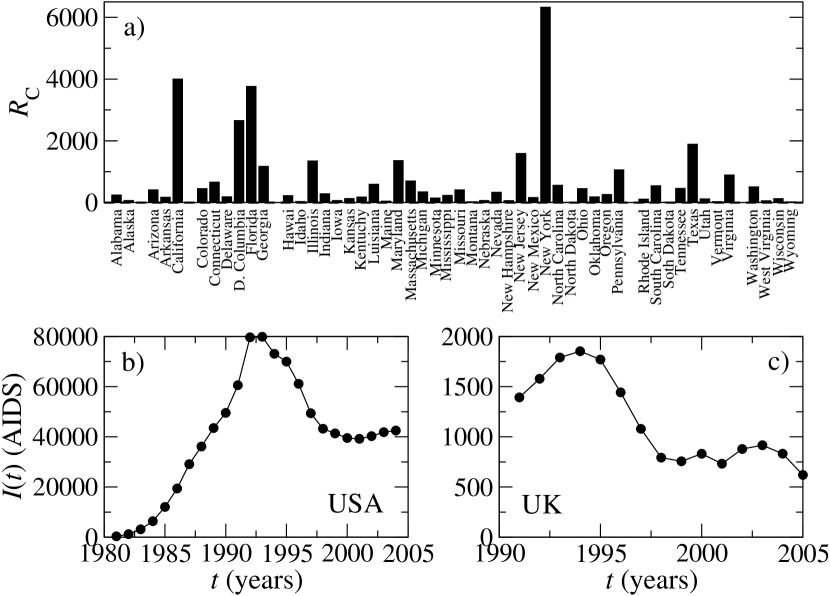
To understand the relevance of these results in a real world scenario I analyze data reported for the AIDS epidemics. First, I estimate the parameter $R_{\rm C}$ determining the spreading regime, local or global. Figure 4a shows the value of $R_{\rm C}$ across the USA by state. For most states $R_{\rm C}>1$, reaching significantly large values for several states. For example, $R_{\rm C}$ exceeds 1,000 for California and New York. These numbers indicate that the USA AIDS epidemics is in the global spread scenario ($R_{\rm C}>1$), in agreement with the general believe.

Second, I analyze the temporal evolution of the AIDS incidence. Fig. 4b and c show the AIDS incidence in USA and UK by year, indicating a similar temporal pattern. The epidemics started with an increasing tendency of the incidence which, after reaching a maximum, switched to a decreasing trend. After some years, however, the epidemics resurges with a new incidence increase. This picture coincides with the model predictions in Fig. 3. Therefore, a possible explanation of the observed multiple peaks is the existence of a community structure, which can be attributed to geographical location and other factors.

Discussion and conclusions

$R_{\rm C}$ in (11) represents the expected number of infected individuals leaving their community. The numerical simulations reported in [Watts et al., 2005] indicated the existence of a transition at $R_{\rm C}=1$, from local outbreaks when $R_{\rm C}<1$ to global epidemics when $R_{\rm C}>1$. I have demonstrated that there is indeed a phase transition at $R_{\rm C}=1$. Furthermore, the analytical solution provides an expression of $R_{\rm C}$ as a function of the bridge’s fraction and the intra-community expected outbreak size (9). $R_{\rm C}$ represents a measure of the reproductive number at the inter-community level. Its value can be estimated from the expected outbreak size inside a community and the bridge’s fraction. Based on the resulting estimate we can determine if an epidemics is in the local or global epidemics scenario and react accordingly.

The inter-community disease transmission is characterized by oscillations at the early stages which represents resurgent epidemics, the number of these resurgencies being determined by the characteristic distance between individuals within a community. In essence, when $D$ is small the time scale characterizing the outbreak progression within a community is very small [Barthélemy et al., 2004, Barthélemy et al., 2005, Vazquez, 2006b]. Therefore, the time it takes to observe the infection of a social bridge is very small as well, resulting in the mixing between the intra- and inter-community transmissions. In contrast, when $D$ is large it takes a longer time to observe the infection of a social bridge and by that time the intra-community outbreak has significantly developed. Therefore, in this last case the outbreak within communities is partially segregated in time.

When multi-agent models are not available these results allow us to evaluate the potential progression of an epidemic outbreak and consequently determine the magnitude of our response to halt it. They are also valuable when a detailed metapolpulation model is available, funneling the search for key quantities among the several model parameters. More important, this work open avenues for future analytical works that side by side with multi-agent models will increase our chances to control global epidemics.

References

  • Anderson & et al, 2004 Anderson, R. M. & et al (2004). Epidemiology, transmission dynamics and control of sars: the 2002-2003 epidemic. Phil. Trans. R. Soc. Lond. B, 359, 1091–1105.
  • Anderson & May, 1991 Anderson, R. M. & May, R. M. (1991). Infectious diseases of humans. Oxford Univ. Press, New York.
  • Barthélemy et al., 2004 Barthélemy, M., Barrat, A., Pastor-Satorras, R. & Vespignani, A. (2004). Velocity and hierarchical spread of epidemic outbreaks in scale-free networks. Phys. Rev. Lett. 92, 178701–178704.
  • Barthélemy et al., 2005 Barthélemy, M., Barrat, A., Pastor-Satorras, R. & Vespignani, A. (2005). Dynamical patterns of epidemic outbreaks in complex heterogeneous networks. J. Theor. Biol. 235, 275–278.
  • Colizza et al., 2006 Colizza, V., Barrat, A., Barthelemy, M. & Vespignani, A. (2006). The role of the airline network in the prediction and predictability of global epidemics. Proc. Natl. Acad. Sci. USA, 103, 2015–2020.
  • Eubank et al., 2004 Eubank, S., Guclu, H., Kumar, V. S. A., Marathe, M., Srinivasan, A., Toroczcai, Z. & Wang, N. (2004). Modelling disease outbreaks in realistic urban social networks. Nature, 429, 180–184.
  • Flahault et al., 1988 Flahault, A., Letrait, S., Blin, P., Hazout, S., Menares, J. & Valleron, A. J. (1988). Modelling the 1985 influenza epidemic in france. Stat. Med. 7, 1147–1155.
  • Germann et al., 2006 Germann, T. C., Kadau, K., Longini, I. M. & Macken, C. A. (2006). Mitigation strategies for pandemic influenza in the united states. Proc. Natl. Acad. Sci. USA, 103, 5935–5940.
  • Hufnagel et al., 2004 Hufnagel, L., Brockmann, D. & T, G. (2004). Forecats and control of epidemics in a globalized world. Proc. Natl. Acad. Sci. USA, 101, 15124–9.
  • Mode, 1971 Mode, C. J. (1971). Multitype branching processes. Elsevier, New York.
  • Riley & et al, 2003 Riley, S. & et al (2003). Transmission dynamics of the etiological agent of sars in hong kong: impact of public health interventions. Science, 300, 1961–1966.
  • Rvachev & Longini, 1985 Rvachev, L. A. & Longini, I. M. (1985). A mathematical model for the global spread of influenza. Math. Biosci. 75, 3–22.
  • Sattenspiel & Dietz, 1995 Sattenspiel, L. & Dietz, K. (1995). A structured epidemic model incorporating geographic mobility among agents. Math. Biosci. 128, 71–91.
  • Vazquez, 2006a Vazquez, A. (2006a). Causal tree of disease transmission and the spreading of infectious diseases. In Discrete Methods in Epidemiology vol. 70, of DIMACS Series in Discrete Mathematics and Theoretical Computer Science pp. 163–179. AMS Providence.
  • Vazquez, 2006b Vazquez, A. (2006b). Polynomial growth in age-dependent branching processes with diverging reproductive number. Phys. Rev. Lett. 96, 038702.
  • Vazquez, 2006c Vazquez, A. Spreading law in a highly interconnected world. http://arxiv.org/q-bio.PE/0603010.
  • Vazquez, 2006d Vazquez, A. Spreading of infectious diseases on heterogeneous populations: multi-type network approach. http://arxiv.org/q-bio.PE/0605001.
  • Watts et al., 2005 Watts, D., Muhamad, R., Medina, D. C. & Dodds, P. S. (2005). Multiscale, resurgent epidemics in a hierarchical metapopulation model. Proc. Natl. Acad. Sci. USA, 102, 11157–11162.