Pattern-based phylogenetic distance estimation
and tree reconstruction

Abstract

We have developed an alignment-free method that calculates phylogenetic distances using a maximum likelihood approach for a model of sequence change on patterns that are discovered in unaligned sequences. To evaluate the phylogenetic accuracy of our method, and to conduct a comprehensive comparison of existing alignment-free methods (freely available as Python package decaf+py at http://www.bioinformatics.org.au), we have created a dataset of reference trees covering a wide range of phylogenetic distances. Amino acid sequences were evolved along the trees and input to the tested methods; from their calculated distances we infered trees whose topologies we compared to the reference trees.

We find our pattern-based method statistically superior to all other tested alignment-free methods on this dataset. We also demonstrate the general advantage of alignment-free methods over an approach based on automated alignments when sequences violate the assumption of collinearity. Similarly, we compare methods on empirical data from an existing alignment benchmark set that we used to derive reference distances and trees. Our pattern-based approach yields distances that show a linear relationship to reference distances over a substantially longer range than other alignment-free methods. The pattern-based approach outperforms alignment-free methods and its phylogenetic accuracy is statistically indistinguishable from alignment-based distances.

Key words: alignment-free methods, phylogenetics, distance estimation, pattern discovery

1 Introduction

Tasks like database searching, sequence classification, phylogenetic tree reconstruction and detection of regulatory sequences are ubiquitous in bioinformatics. Most methods performing these tasks are based on (automated) alignments; however, alignment-free methods exist for solving the tasks. Recent years have seen an increasing number of alignment-free methods (reviewed in ?, ?, see also ?, ?; ?, ?; ?, ?; ?, ?; ?, ?; ?, ?). In contrast to methods based on (automated) alignments, alignment-free methods make fewer assumptions about the nature of the sequences they work on, and so far are mostly devoid of any evolutionary model of sequence change (the only exception being the W-metric by ?, ?). The absence of an assumption of collinearity over long stretches (implicit in any alignment) destines them to be especially useful for handling DNA sequences that have undergone recombination, proteins with shuffled domains, and genomic sequences (which often feature large-scale rearrangements).

Previously, several alignment-free methods have been compared systematically for classification purposes and their ability to detect regulatory sequences. However, surprisingly little is known about their accuracy in phylogeny reconstruction. So far, most new methods have been verified on a few trees only. A systematic study is sorely lacking in this field of research.

In Section 2 below we describe several alignment-free methods that we included in our comparison. We propose a new alignment-free method based on patterns in sequences, and a variant thereof, in Section 3. The phylogenetic accuracy of these methods is comparatively evaluated on synthetic and empirical data, covering a wide range of phylogenetic distances, and we assess whether differences are statistically significant in Section 4 before presenting conclusions.

2 Previous work

In this section, we provide a summary of previously established alignment-free methods. Some methods were reviewed in ? (?), while others are more recent and are compared here for the first time.

We represent a biological sequence by a string $X$ of $n$ characters taken from the alphabet $\mathcal{A}$ which contains $c$ different characters $\{a_{1},\dots,a_{c}\}$, e.g. all amino acids. Most alignment-free methods operate on words of length $k$, so-called $k$-mers: there are $w=c^{k}$ such different words. We represent the set of $k$-mers in $X$ (or a derived property) by vector $\mathbf{v}^{X}=(v^{X}_{1},\dots,v^{X}_{w})$; the parameter $k$ is always implied. Each vector element describes the abundance of $k$-mer $i$.

The (squared) Euclidean distance was introduced into sequence comparison by ? (?). The distance between $X$ and $Y$ is calculated using $c^{X}_{i}$, the count of $k$-mer occurrences in $X$.

$$d^{E}(X,Y)=\sum_{i=1}^{w}\left(c^{X}_{i}-c^{Y}_{i}\right)^{2}$$ (1)

Later, ? (?) found that $d^{E}$ yields values about twice the number of mismatch counts obtained from alignments.

The standardized Euclidean distance was found to improve on $d^{E}$ without incurring the computational problems associated with the slightly better performing Mahalanobis distance (?, ?).

$$d^{S}(X,Y)=\sum_{i=1}^{w}\left(f^{X}_{i}/s^{X}_{i}-f^{Y}_{i}/s^{Y}_{i}\right)^{2}$$ (2)

Divide $f^{X}_{i}$, the relative frequencies of $k$-mer occurrences in $X$, by their standard deviations $s^{X}_{i}$ as calculated from a set of equilibrium frequencies (?, ?).

? (?) described the fractional common $k$-mer count; it is used in a distance measure that speeds up guide tree construction in MUSCLE (?, ?). Let $C^{XY}_{i}=\min(c^{X}_{i},c^{Y}_{i})$ denote the common $k$-mer count, and $Y$ be a string with $m$ characters.

$$F(X,Y)=\sum_{i=1}^{w}C^{XY}_{i}/[\min(n,m)-k+1]$$ (3)

$$d^{F}(X,Y)=-\log(\epsilon+F)$$ (4)

$F$, the fraction of common $k$-mers between $X$ and $Y$, ranges from 0 to 1 and $d^{F}$ transforms this into a distance: $\epsilon$, a small value added to prevent taking the logarithm of zero (at least in ?, ?), is 0.1 there but 0.02 in MUSCLE. Both versions employ $d^{F}$ in slightly different ways; here, we directly use this common basis with $\epsilon=0.1$.

? (?) compared several metrics for their suitability in classifying genes based on their regulatory sequences. He found a similarity measure based on probabilities from common $k$-mer counts under a multiplicative Poisson model to be best-performing. In our adaptation, we directly use the probabilities from Equation 5 without transforming them into similarities.

$$P\negmedspace\left(x\geq C^{XY}_{i}\right)=\begin{cases}\left[1-F^{P}\negthickspace\left(C^{XY}_{i}-1,E_{i}\right)\right]^{2}&\text{if $C^{XY}_{i}>0$,}\\ 1&\text{else.}\end{cases}$$ (5)

$$d^{P}(X,Y)=\biggl{[}\prod_{i=1}^{w}P\negmedspace\left(x\geq C^{XY}_{i}\right)\biggr{]}^{1/w}$$ (6)

Here, in the calculation of $C^{XY}_{i}$ the occurrence counts of $k$-mers are filtered to remove self-overlapping instances, thereby justifying the Poisson assumption. $F^{P}$ refers to the Poisson probability distribution function and its parameter $E_{i}$ is the expected count under a set of equilibrium frequencies. $P(x\geq C^{XY}_{i})$ is the probability that we observe a $k$-mer count at least as high as that between $X$ and $Y$.

The last word-based alignment-free method considered here is the composition distance of ? (?). Under a Markov model of order $k-2$ we predict the probability $p^{0}$ of a word (the $c_{i}$ refer to its characters) from the probabilities of appropriate shorter subwords, respective their relative frequencies. To get the expected count $E^{X}$ of a $k$-mer in $X$, we re-arrange the corresponding total numbers.

$$p^{0}(c_{1},\dots,c_{k})\equiv\frac{p(c_{1},\dots,c_{k-1})p(c_{2},\dots,c_{k})}{p(c_{2},\dots,c_{k-1})}$$ (7)

$$E^{X}(c_{1},\dots,c_{k})=\frac{c^{X}(c_{1},\dots,c_{k-1})c^{X}(c_{2},\dots,c_{k})}{c^{X}(c_{2},\dots,c_{k-1})}\cdot\frac{(n-k+1)(n-k+3)}{(n-k+2)^{2}}$$ (8)

We can now assemble the composition vector (?, ?) for $k$-mer occurrence counts $c^{X}$ in $X$: $\mathbf{v}^{X}=(\mathbf{c}^{X}-\mathbf{E}^{X})/\mathbf{E}^{X}$. Then we calculate the correlation between $X$ and $Y$ as the cosine of the angle between their composition vectors, and obtain a normalized dissimilarity $d^{C}$.

$$\cos(X,Y)=\frac{\sum_{i=1}^{w}v^{X}_{i}v^{Y}_{i}}{\left[\sum_{i=1}^{w}(v^{X}_{i})^{2}\times\sum_{i=1}^{w}(v^{Y}_{i})^{2}\right]^{1/2}}$$ (9)

$$d^{C}(X,Y)=\frac{1-\cos(X,Y)}{2}$$ (10)

The W-metric due to ? (?) is “word-based” but operates on 1-mers only:

$$d^{W}(X,Y)=\sum_{i=1}^{w}\sum_{j=1}^{w}(f^{X}_{i}-f^{Y}_{i})\cdot(f^{X}_{j}-f^{Y}_{j})\cdot W_{ij}$$ (11)

Differences in amino acid composition, $f^{X}_{i}-f^{Y}_{i}$, between all pairs of amino acids, are weighted by their entries in matrix $\mathbf{W}$. ? (?) found their results virtually the same for different scoring matrices (BLOSUM62, BLOSUM50, BLOSUM40 and PAM250); we use BLOSUM62 (?, ?).

? (?) showed how Lempel-Ziv complexity, computed in a simple fashion utilizing two elementary operations (?, ?), can be used to define distance measures. We examine their final measure (that they call d${}_{1}^{**}$): $c(X)$ denotes the Lempel-Ziv complexity of $X$, and $XY$ refers to the concatenation of $X$ and $Y$.

$$d^{LZ}(X,Y)=\frac{c(XY)-c(X)+c(YX)-c(Y)}{\frac{1}{2}\bigl{[}c(XY)+c(YX)\bigr{]}}$$ (12)

Most recently, ? (?) proposed the Average Common Substring (ACS) approach. They define $L(X,Y)=\sum_{i=1}^{n}\ell^{XY}_{i}\negmedspace/n$, where $\ell^{XY}_{i}$ is the length of the longest string starting at $X_{i}$ that exactly matches a string starting at $Y_{j}$. $L$ provides a normalized length measure, from which we obtain an intermediate (asymmetric) distance $d$ and finally $d^{ACS}$.

$$d(X,Y)=\frac{\log(m)}{L(X,Y)}-\frac{\log(n)}{L(X,X)}$$ (13)

$$d^{ACS}(X,Y)=\frac{1}{2}\bigl{[}d(X,Y)+d(Y,X)\bigr{]}$$ (14)

3 Pattern-based approach

We use pattern discovery to find regions of similarity (presumed homology) occurring in two or more sequences; no alignment is necessary. To estimate phylogenetic distances, the patterns are considered to be local alignments. Adopting this point of view enables us to apply an established maximum likelihood (ML) approach. Both the application of pattern discovery, and distance estimation by ML, represent novel steps in this context. We infer pairwise distances from the sequence data covered by patterns, yielding a distance matrix. Distance-based tree inference then proceeds by conventional means.

3.1 Terminology

We briefly introduce some basic terminology for TEIRESIAS; for more details, including a description of the algorithm, the reader is referred to (?, ?). Let $\mathcal{A}$ denote the alphabet of characters, e.g. all amino acids. Let ${}^{\prime}.^{\prime}\not\in\mathcal{A}$ be the wildcard character that represents any amino acid. Define a pattern $P$ to be the regular expression $\mathcal{A}(\mathcal{A}\cup\{^{\prime}.^{\prime}\})^{*}\mathcal{A}$. A subpattern of $P$ is any substring that is a pattern. Call $P$ a $<\!L,W\!>$ pattern ($L\leq W$) if any subpattern of length $\geq W$ has $\geq L$ characters $\in\mathcal{A}$. A pattern $P$ has support $K$ if it occurs (has instances) in $K$ sequences. A pattern $P$ can be made more specific by replacing wildcard characters by characters $\in\mathcal{A}$ and/or extending $P$ to the left or right. Call $P$ maximal with respect to a sequence set $S$ if making $P$ more specific reduces its total support (irrespective of the number of sequences).

We are now ready to state the behaviour of the algorithm: TEIRESIAS finds all maximal $<\!L,W\!>$ patterns (with support $\geq K$) in a set $S$ of unaligned sequences.

3.2 Distance calculation

The pairwise distance $d^{PB}$ between two sequences $S_{i}$ and $S_{j}$ is computed as follows: first, we filter out patterns that occur more than once in any sequence. This removes false positives and ensures that the self-distance of any sequence is zero. Second, all instances of patterns occurring simultaneously in (at least) $S_{i}$ and $S_{j}$ are concatenated, resulting in two new sequences $S^{\prime}_{ij}$ and $S^{\prime}_{ji}$ of the same length. Note that a pattern may occur in three or more sequences, in which case we project it on multiple pairs of sequences. Also note that generally $S^{\prime}_{ij}$ (and $S^{\prime}_{ji}$) will differ in length from $S^{\prime}_{ik}$ (and $S^{\prime}_{ki}$) because the patterns occurring simultaneously in (at least) $S_{i}$ and $S_{j}$ will differ in number (and number of residues they cover) from those appearing in $S_{k}$ and $S_{j}$. Third, these new, concatenated sequences are used to estimate pairwise distances. This is done by applying a maximum likelihood-based approach that optimizes with respect to a model of amino acid evolution. For the purpose of this work we use the JTT model (?, ?) as implemented in Protdist from the PHYLIP package (?, ?).

Note that the algorithm for calculating distances from patterns is general. Our means for pattern discovery is TEIRESIAS, but, in principle at least, other tools could also be used (eg ?, ?). To retain the alignment-free property of our approach, any replacement needs to have that property as well.

3.3 Parametrization

Our rationale for parameterizing TEIRESIAS with $L=4$, $W=16$ is as follows. Consider ordinary $k$-mers: higher values for $k$ reduce chance occurrences among a set of sequences, thus reducing false positives. We observe that TEIRESIAS patterns and $k$-mers bear a relationship; to this end we introduce elementary patterns: an elementary pattern is a $<\!L,W\!>$ pattern with exactly $L$ residues. TEIRESIAS discovers maximal $<\!L,W\!>$ patterns using elementary patterns as building blocks during its convolution phase (?, ?). For the special case $W=L$ (no wildcard characters are allowed), we find that setting $L=k$ leads to elementary patterns capturing a subset of all $k$-mers. The only difference is that $K=1$ for $k$-mers (a $k$-mer may occur only once) whereas we use $K=2$ for TEIRESIAS (a pattern must occur in at least two sequences). Thus we see that higher values for $L$ reduce the number of false positives. For our distance calculation, however, we need patterns capable of accounting for differences between sequences, hence we require $W>L$. In preliminary experiments on data described in Section 4.2, we tried several higher values for $L$ with $W>L$ first. We found for $L=4$, $W=16$ (a ratio of $L/W=0.25$), the values that we use throughout Section 4, all pairwise distances are defined, i.e. every pair of sequences is covered by at least one instance of a pattern. For $W=8$, corresponding to a ratio of $L/W=0.5$, and higher values of $W$, approaching the ratio $L/W=0.25$, the number of undefined distances is 229, 127, 63, 32, 23, 8, 5, and 2 out of 8667. (On data from Section 4.1, all distances are defined for $W=8$.)

Undefined distances point towards a problem: some sequence pairs are too divergent—no pair of substrings can be described by (elementary) $<\!L,W\!>$ patterns. The ratio $L/W$ determines the minimum similarity any subpattern must possess: it effectively specifies a local similarity threshold. Thus, undefined distances mean that no pair of substrings reach or exceed this threshold. Our solution to the problem is to make sequences more similar by encoding them in a reduced alphabet. Following ? (?) and earlier work by ? (?), we choose a reduction based on chemical equivalences: [AG], [DE], [FY], [KR], [ILMV], [QN], [ST], [BZX] where ’[…]’ groups similar amino acids together, and unlisted amino acids form classes of their own. The phylogenetic distance calculation is based on the original sequence data covered by the resulting patterns; this usually improves phylogenetic accuracy (see Section 4.1.1 and 4.2.2). As a result of encoding sequences, all pairwise distances for e.g. $L=4$, $W=8$ are defined.

We also find that for sufficiently small values of $L$, the phylogenetic accuracy is virtually independent of the particular choice of $L$, and largely depends on the ratio $L/W$ (data not shown). Generally, the accuracy of tree reconstruction improves as the local similarity threshold is lowered, with diminishing improvement and higher computational costs the further it is lowered.

3.4 Majority consensus and consistency

One property of TEIRESIAS is that each residue can (and given our parametrization, usually will) participate in multiple patterns. This may lead to situations where a particular residue in one sequence pairs with two or more different residues in a second sequence. It is not clear how this should be interpreted with respect to homology. We propose a variant, $d^{PBMC}$ that resolves this conflict by way of (relative) majority consensus and consistency. We discover patterns as before but introduce an intermediate step before distance estimation. We record paired positions across all patterns. For any two sequences $S_{i}$ and $S_{j}$, we take positions $(p_{i},p_{j})$ if and only if a) $p_{i}$ is paired with $p^{\prime}_{j}$ more often than with any other position in $S_{j}$, b) $p_{j}$ is paired with $p^{\prime}_{i}$ more often than with any other position in $S_{i}$, and c) $p_{i}=p^{\prime}_{i}$ and $p_{j}=p^{\prime}_{j}$, i.e. the positions are the same. This ensures that every residue participates at most once for a given sequence pair in the distance calculation step. For parameters $L=4$, $W=16$, the constraints prove to be stringent and discard most of the data.

4 Comparison of alignment-free methods

4.1 Synthetic data

We use a birth-death process to model cladogenesis (?, ?) and sample from several tree distributions. The effects of different taxon sampling strategies are described in (?, ?). Trees resulting from a birth-death process are rooted, bifurcating and ultrametric; we deviate them from ultrametricity by an additive process to keep the expectation of the phylogenetic distances unchanged.

Using PhyloGen V1.1 (?, ?) we sampled seven sets of 100 four-taxon reference trees each; the parameters were $\texttt{birth}=10.0$ and $\texttt{death}=5.0$, with $\texttt{extant}\in[40,133,\dots,40000]$ corresponding to a sample fraction of $[0.1,0.03,\dots,0.0001]$. The induced pairwise phylogenetic reference distances have medians of $[0.71,1.11,1.61,2.08,2.46,2.96,3.39]$ substitutions per site; their upper and lower quartiles are within $0.35$ units of these values. For later use, we label the first, fourth and last set as having small, medium and large phylogenetic distances. Sequences were evolved along the branches of the deviated trees using SEQ-GEN (?, ?) V1.3.2 under the JTT model (?, ?), and for a sequence length of 1000 amino acids. (Where possible, we parameterized alignment-free methods with the JTT model, or its equilibrium frequencies.)

To compare alignment-free methods with alignment-based methods when the assumption of collinearity is violated, we constructed an additional dataset with a wide distribution of phylogenetic distances. We sampled one four-taxon tree each from 100 different distributions specified by sample fractions that varied evenly on a logarithmic scale. The induced pairwise phylogenetic reference distances have a median of 1.77 substitutions per site; the upper and lower quartiles are 2.54 and 1.02, respectively, and the maximum is 4.88. Sequences of length 1000 were evolved as before, and for every sequence set the first and last halves of two sequences were exchanged. This corresponds to a recent domain shuffle event. We deliberately chose an extreme example to show the severity that a non-justified assumption of collinearity can have.

The generated sequences were input to the tested alignment-free methods, and the resulting test distances were used to infer neighbor-joining (NJ: ?, ?) trees. Phylogenetic accuracy is measured by the Robinson-Foulds (RF: ?, ?) tree metric. We compute the topological difference between a test tree and its corresponding (unrooted) reference tree, and report results for each set. To assess the statistical significance of differences between methods we employ the Friedman test (corrected for tied ranks), followed by Tukey-style posthoc comparisons if a significant difference is found (see e.g. ?, ?).

4.1.1 Phylogenetic accuracy

Here, and in Section 4.2.2 we are interested in the accuracy of methods in reconstructiong the phylogentic relationships among a set of sequences; we refer to this quantity as phylogenetic accuracy for short. We measure and report the topological differences between test and reference trees: better methods yield fewer differences, and hence have a higher accuracy. When we assess methods based on their ranksums of the Friedman test, better methods obtain lower numbers and rank first.

Influence of k and alphabet

Here, we look at the performance of word-based alignment-free methods as a function of the length of $k$-mers and the alphabet in use. We varied $k$ from 1 to 9 where possible: the composition distance requires a minimum of $k=3$. The alphabet consisted of either the original amino acids (AA) or the chemical equivalence classes (CE) from Section 3.3.

For AA sequences, word length $k=4$ performs best for methods $d^{E}$, $d^{S}$, $d^{F}$ and $d^{P}$ as judged by their ranksums based on phylogenetic accuracy over all seven reference sets. Second- and third-ranking word lengths for $d^{E}$ and $d^{P}$ are $k=5$ and $k=3$. For $d^{F}$ these lengths have tied ranks, and for $d^{S}$ this order is reversed. Method $d^{C}$ performs best for $k=3$, with $k=4$ ($k=5$) ranking second (third).

For CE sequences, slightly higher values for $k$ yield lower ranksums. Methods $d^{E}$, $d^{F}$ and $d^{P}$ perform best with word length $k=5$. Second- and third-ranking word lengths for $d^{E}$ and $d^{P}$ are $k=6$ and $k=7$, for $d^{F}$ this order is reversed. For $d^{S}$, word lengths $k=5$ and $k=6$ rank equal best, followed by $k=4$. Again, method $d^{C}$ shows a preference for lower values: it performs jointly best for $k=4$ and $k=5$, followed by $k=3$.

What we have described so far is based on the ranksums over all seven reference sets spanning the relevant space of phylogenetic distances for tree inference. Looking at the phylogenetic accuracy of word-based methods on individual sets with narrow distributions of phylogenetic distances reveals a more complex picture. As expected, the topological difference between test and reference trees increases with increasing phylogenetic reference distances. However, depending on the choice of $k$, the absolute values of this difference may vary considerably. This leads to a number of curves with different shapes when plotting the accuracy for a particular method on the the Y-axis with the X-axis showing values for $k$ (Figure 1). We find that overall, the choice of method has less impact on the shape of these curves than does phylogenetic distance. Comparing AA with CE sequences shows similarly shaped curves that are shifted to the right for CE.

Figure 1 (a,c,e) shows curves for method $d^{E}$ for three out of seven different reference sets with small, medium and large phylogenetic distances. The curves for methods $d^{S}$, $d^{F}$ and $d^{P}$ are similar and omitted here. The curve for medium distances corresponds to our overall findings. Small and large distances hint at a better performance for small values of $k$. Inspection of these plots for the remaining methods fails to identify a single best $k$. Figure 1 (b,d,f) for $d^{C}$ reveals some striking peculiarities of this method. In these three sets, the topological difference for $k=6$ is often the highest, even though the neighbor value $k=5$ may yield a low topological difference (medium distances): thus the parameter space is uneven, more so than for other methods.

Taken together, these results indicate that, depending on the phylogenetic distance of the sequences, the word length most appropriate for analysis of a particular dataset may well be different from the one performing best over all sets tested here.

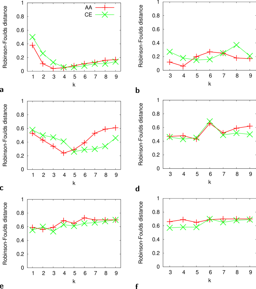
Figure 1: Average Robinson-Foulds distance (Y-axis) for two methods (a,c,e: $d^{E}$; b,d,f: $d^{C}$) on three reference sets (top to bottom: small, medium and large phylogenetic distances). Each subfigure shows the behaviour as a function of $k$ (X-axis) under two alphabets (AA: original amino acids, CE: chemical equivalence classes). Points are joined for ease of visual inspection only.

Statistical significance

Here, we conduct a comprehensive comparison of all methods: we show their phylogenetic accuracy and assign statistical significance to our findings. For $k$-mer-based methods, we select the best-performing word lengths on the two alphabets as described above. We compare these methods to $d^{ACS}$, $d^{LZ}$ and $d^{W}$, and to two variants of the pattern-based approach: $d^{PB}$ and $d^{PBMC}$. As a baseline, we include $d^{ML}$, the maximum likelihood (ML) estimate of phylogenetic distances between the (already correctly aligned) sequences.

Table 1 lists selected methods in ranksum order based on all 700 trees, from best to worst. For every method, we show the number of incorrectly reconstructed trees in each of the seven sets. Recall that unrooted, bifurcating four-taxon trees can be reconstructed either correctly or incorrectly: the RF distance will be 0 or 1, with no intermediate values possible.

					Synthetic reference set
#	Ranksum	Method	$\mathcal{A}$	$k$	1	2	3	4	5	6	7
1	5640.0	$d^{ML}$	AA	–	2	2	7	12	13	18	17
2	6058.0	$d^{PB}$	CE	–	3	2	10	9	19	29	43
3	6390.5	$d^{PBMC}$	CE	–	3	3	10	10	23	42	59
4	6523.5	$d^{PB}$	AA	–	4	2	7	18	38	45	50
5	6951.0	$d^{S}$	CE	5	8	6	19	27	45	47	57
6	6960.5	$d^{P}$	AA	4	8	1	14	24	44	50	69
7	6970.0	$d^{E}$	AA	4	5	2	17	24	46	48	69
8	6989.0	$d^{ACS}$	AA	–	9	3	17	24	49	52	59
9	6998.5	$d^{P}$	CE	5	7	4	18	30	47	49	59
10	7036.5	$d^{S}$	AA	4	8	8	20	31	43	46	62
11	7036.5	$d^{F}$	AA	4	9	2	14	24	48	50	71
12	7055.5	$d^{E}$	CE	5	6	7	21	26	51	48	61
13	7065.0	$d^{ACS}$	CE	–	10	7	21	30	43	55	55
14	7074.5	$d^{F}$	CE	5	6	6	21	31	47	49	62
15	7359.5	$d^{LZ}$	CE	–	6	5	28	39	49	66	59
16	7378.5	$d^{LZ}$	AA	–	3	8	21	34	53	64	71
17	7597.0	$d^{C}$	AA	3	12	14	31	47	49	58	66
18	7635.0	$d^{C}$	CE	5	15	14	32	45	54	63	58
19	8281.0	$d^{W}$	AA	(1)	43	34	35	55	50	71	61

Table 1: Shown are the number of incorrectly reconstructed trees (out of 100) for each synthetic reference set and method. The order is based on ranksums; for each word-based method (and alphabet $\mathcal{A}$), we include the best-performing $k$ (method $d^{W}$ can only take on a value of 1).

The test statistic of the Friedman test (corrected for tied ranks) is $F_{R}=709.6$ ($N=700$, $k=19$). This is highly significant ($P<10^{-10}$) beyond the $\alpha=0.05$ level. Significant differences are found between the following pairs (numbers refer to column ’#’ of Table 1): method 1 vs methods 19–4, method 2 vs methods 19–5, methods 3 and 4 vs methods 19–15, and methods 5–16 vs method 19. Thus the performance of most alignment-free methods as tested here is statistically indistinguishable from one another. The ranksums of methods 5–14 range from 6951.0 to 7074.5, differing by $\leq 123.5$. However, the pattern-based method $d^{PB}$ with CE, $L=4$, $W=16$ (ranksum: 6058.0) is significantly better than all alignment-free methods not based on patterns. The ML estimate based on the correct alignment, $d^{ML}$, is significantly better than all traditional alignment-free methods and the pattern-based method working on original AA sequences. Our tests show that $d^{ML}$ is not significantly better than the two best-performing pattern-based variants working on CE sequences.

By far the worst method tested here is the W-metric $d^{W}$ (ranksum: 8281.0): differences to nearly all other methods are significant. The lack of phylogenetic accuracy originates from being based on 1-mers. For comparison, $d^{E}$ with AA, $k=1$ incorrectly reconstructs the following number of trees for the seven reference sets: 38, 30, 39, 53, 58, 66, 59. These numbers are quite similar to the ones in Table 1, as are the numbers for equally parameterized methods $d^{S}$ and $d^{F}$. In the case of $d^{P}$, however, they are 59, 56, 65, 75, 59, 71, 65. This is an artifact of the method for $k=1$ (and to some extent for $k=2$) and vanishes for higher values. Also apparent is the poor performance of both parametrizations of $d^{LZ}$ and $d^{C}$, the Lempel-Ziv and composition distances, respectively, with ranksums between 7359.5 and 7635.0.

Domain shuffling

We now describe our findings from the reference set with simulated domain shuffling data. We apply the same alignment-free methods with parameter settings as before on the unaligned, partly shuffled sequences. Additionally, we run a number of multiple sequence alignment (MSA) programs on this data (?, ?, ?, ?, ?), and estimate ML distances from these alignments ($d^{\textsc{ClustalW}}$, $d^{\textsc{Dialign}}$, $d^{\textsc{MUSCLE}}$ and $d^{\textsc{ProbCons}}$, respectively). This corresponds to an undesirable situation where e.g. in an automated environment tests have failed to detect the presence of domain shuffling. Hence, distances are estimated from alignments where not all homologous residues can possibly be aligned, and it is likely that in fact a substantial fraction of non-homologous residues have been aligned.

The Friedman test ($F_{R}=270.3$, $N=100$, $k=22$) detects the presence of a difference that is highly significant ($P<10^{-10}$) beyond the $\alpha=0.05$ level. However, pairwise differences are statistically significant only between $d^{\textsc{ClustalW}}$ and all other methods; this is likely due to lack of statistical power. Two parametrizations (CE and AA) of the pattern-based method $d^{PB}$, $L=4$, $W=16$, rank jointly first with ranksums of 1011.5: they reconstruct 11 out of 100 trees incorrectly. This is followed jointly by $d^{PBMC}$, with CE, $L=4$, $W=16$, and $d^{S}$ and $d^{F}$, both with CE, $k=5$. Their ranksums are 1066.5, and they reconstruct 16 trees incorrectly. The numbers for alignment-based approaches are as follows (ranksum in parentheses): $d^{\textsc{ClustalW}}$: 71 (1671.5), $d^{\textsc{MUSCLE}}$: 28 (1198.5), $d^{\textsc{ProbCons}}$: 25 (1165.5), and $d^{\textsc{Dialign}}$: 21 (1121.5). Three out of four alignment-based approaches are among the seven worst-ranking methods. Interestingly $d^{\textsc{Dialign}}$, the best-performing of these approaches, uses a local alignment strategy; it occupies rank eleven jointly with two other methods. Conversely, what we just described means that e.g. $d^{LZ}$, working on AA sequences, one of the worst-performing alignment-free methods as tested here, has a higher phylogenetic accuracy than three out of four combinations of MSA program and ML estimate, and even $d^{W}$ is significantly better than $d^{\textsc{ClustalW}}$ on this data. Overall, the results show that alignment-free methods may perform better than alignment-based approaches, especially on non-collinear sequence data, as alignment-free methods do not make assumptions of collinearity.

4.2 Empirical data

We use the data from version 2 of the original BAliBASE sets (?, ?). They consist of 141 manually curated benchmark alignments that are organized in five reference sets. Their purpose is to support tests of alignment tools under a variety of conditions: Set 1 is made up of roughly equi-distant sequences that are divided into nine subsets according to their sequence conservation and alignment length. Set 2 contains sequence families that are aligned with a highly divergent orphan sequence. Set 3 aligns subgroups with less than 25 percent identity between them. Set 4 consists of sequences with N- or C-terminal extensions, i.e. the sequences are not trimmed at alignment boundaries. Set 5 is complementary to set 4: some sequences contain internal insertions. Two alignments contain only three sequences each and are not considered for evaluation of phylogenetic accuracy, as there is only one corresponding unrooted tree topology. The remaining 139 alignments consist of between 4 and 28 sequences each.

For each reference alignment, we estimate phylogenetic reference distances using Protdist, and reconstruct both neighbor-joining (NJ) and Fitch-Margoliash (FM: ?, ?) reference trees. The topological difference between a test tree and its corresponding reference tree is measured by the Robinson-Foulds (RF) and the Quartet (Q) distance (?, ?; implemented in QDist: ?, ?). As these are empirical data, we cannot know the true tree along which the sequences evolved; however, we find that by using a large number of trees, and four combinations of tree reconstruction method and tree topology metric (RF-NJ, RF-FM, Q-NJ, Q-FM), we are able to rank methods robustly. Statistical significance is assessed as in Section 4.1.

4.2.1 Phylogenetic distances

Here, we inspect the behaviour of pairwise phylogenetic distances. The BAliBASE alignments yield 8667 reference distances, of which $<2.5\%$ have $\geq 5.0$ substitutions per site (36 distances are $\geq 10.0$). In what follows, we consider reference distances $<5.0$, i.e. $<500$ PAMs. Note that “distances of 250–300 PAM units are commonly considered as the maximum for reasonable distance estimation” (?, ?). Figure 2 contains scatterplots where the X-axis refers to the afore-mentioned reference distances. The Y-axis shows the corresponding phylogenetic distances obtained using selected alignment-free methods with original AA sequences (and, if the methods are word-based, values for $k$ as in Table 1). Additionally, we show distances obtained from CE sequences where the distribution differs noticably.

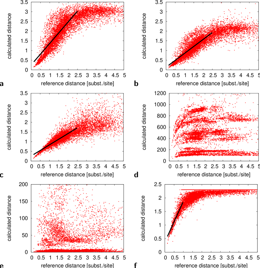
Figure 2: Pairwise phylogenetic reference distances (X-axis) plotted against corresponding calculated distances (Y-axis). Methods and parameters are as follows: a) $d^{PB}$ with $L=4$, $W=16$, CE, b) $d^{PB}$ with $L=4$, $W=16$, AA, c) $d^{PBMC}$ with $L=4$, $W=16$, CE, d) $d^{E}$ with $k=4$, AA, e) $d^{S}$ with $k=4$, AA, f) $d^{F}$ with $k=4$, AA (cont’d).

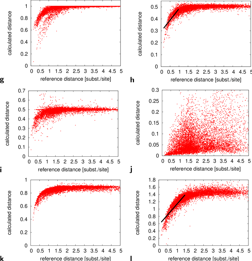
Figure 2: (cont’d) g) $d^{P}$ with $k=4$, AA, h) $d^{C}$ with $k=3$, AA, i) $d^{C}$ with $k=5$, CE, j) $d^{W}$, k) $d^{LZ}$ with AA, l) $d^{ACS}$ with AA.

Figure 2a for $d^{PB}$ with CE sequences, $L=4$, $W=16$, shows a linear relationship between reference and estimated distances for up to about 2.5 substitutions per site. Linear regression for all points below this cutoff yields $y=0.2598+1.1092x$ with a correlation coefficient (CC) of 0.8188. Higher distances are increasingly underestimated as saturation comes into effect and limits most distances ($>99\%$) to values $<3.5$.

When patterns are discovered using the original BAliBASE sequences (Figure 2b) as opposed to using CE, the resulting distances are approximated by a line with a lesser slope ($y=0.1373+0.7160x$, CC$=0.8261$); saturation limits most distances ($>99\%$) to values $<2.5$. For the variant $d^{PBMC}$ with CE sequences, $L=4$, $W=16$ (Figure 2c), the linear relationship extends at least up to 2.5 substitions per site and the slope is roughly half that of the equally parameterized $d^{PB}$ ($y=0.2535+0.5819x$, CC$=0.8564$). Again, most distances ($>99\%$) are limited to values $<3.5$, however this curve shows less saturation and more scatter.

The (squared) Euclidean distance $d^{E}$ does not yield values that can be interpreted in units of substitutions per site. Instead, they relate to mismatch counts (?, ?) and are therefore sequence length-dependent. Correspondingly, the distances do not show a single discernable linear relationship (Figure 2d for $k=4$, with AA sequences). Most of the data ($>99\%$) have an Euclidean distance of $<1200$; data for $k=5$, with CE sequences are very similar and omitted here.

Similarly, $d^{S}$ has no single discernable linear relationship, with most data ($>99\%$) taking on numerical values of $<200$ ($k=4$, AA, Figure 2e). However, parameters $k=5$, CE yield distances with most values ($>99\%$) being $<4000$, although the scatterplots look almost identical.

We find a linear relationship between reference and $d^{F}$ distances for up to about 1.0 substitutions per site (Figure 2f). Linear regression for all points below this cutoff yields $y=0.3681+1.5088x$, CC$=0.8626$. We find 25.5% of all pairwise distances are $-\log(\epsilon)$, i.e. would be undefined without adding $\epsilon$ as no $k$-mer is common to a sequence pair. This problem occurs especially for short, divergent sequences in set 1 of BAliBASE. For $k=5$, with CE sequences, this number drops down considerably to 15.1%, and the plot exhibits more scatter.

A similar problem occurs for $d^{P}$ (Figure 2g), which is also based on common $k$-mers. Here 30.8% of all pairwise distances yield the value 1.0; this higher percentage is possibly caused by numerical instabilities when multiplying small probablilities. As before, parametrization with $k=5$, CE reduces the percentage considerably, to 21.0%, and increases scatter.

The scatterplots for the composition distance $d^{C}$ differ between parametrization $k=3$, AA and $k=5$, CE (Figure 2h,i). The former version shows a linear behaviour for up to about 1.0 substitutions per site ($y=0.2946+0.1906x$, CC$=0.7881$), with no value $\geq 0.55$, whereas the latter version shows no such large linear behaviour and is limited to about $0.75$. More importantly, in this latter version 13.1% of its distances are exactly 0.5 (within the usual precision limits imposed by implementations of floating point numbers), and 30.2% are $\in[0.4999,0.5001]$. For the former version, just 6 distances amount to 0.5, and 60 are $\in[0.4999,0.5001]$.

We find no discernable relationship between reference distances $>0.5$ and distances produced by the W-metric (Figure 2j). This likely explains why it turns out to be the worst of all tested methods here. The distances are mostly ($>99\%$) limited to values $<0.3$.

The two distributions of values for parametrizations of the Lempel-Ziv distance $d^{LZ}$ with both AA (Figure 2k) and CE sequences are very similar, with CE showing more scatter.

The method $d^{ACS}$ shows a linear relationship between reference and calculated distances for up to about 1.0–1.5 substitutions per site (Figure 2l). Linear regression for all points below 1.5 yields $y=0.5618+0.5631x$ (CC$=0.8643$). We find most distances ($>99\%$) are limited to values $<1.65$. For CE sequences, most distances ($>99\%$) are limited to values $<1.1$.

Comparing the various distributions, we find that all three versions of our pattern-based approach yield pairwise distances that exhibit a linear relationship to phylogenetic reference distances for up to about 2.5 substitutions per site. This constitutes a considerable increase from a maximum of 1.0–1.5 substitutions per site for methods $d^{ACS}$, $d^{F}$ and $d^{C}$. The linear relationship is a desirable property, and likely explains the higher phylogenetic accuracy of the pattern-based approach.

4.2.2 Phylogenetic accuracy

Statistical significance

Table 2 lists selected alignment-free methods and four approaches based on the ML distance estimate from automated alignments. To obtain combined ranksums for statistical analysis, we average the normalized topological differences over all four combinations of tree reconstruction method and tree distance measure (RF-NJ, RF-FM, Q-NJ, Q-FM) based on 139 sequence sets. The combined ranksums range from 975.5 to 2338.0. This is a slightly wider range than for each individual combination, for which the extreme values are $\in[987.5,1058.5]$ and $\in[2280.0,2312.0]$. The first and last six methods are ranked identically between the combined analysis and combination RF-NJ. The average normalized topological differences for this combination are shown in Table 2 for all five BAliBASE reference sets.

					BAliBASE reference set
#	Ranksum	Method	$\mathcal{A}$	$k$	1	2	3	4	5
1	975.5	$d^{\textsc{MUSCLE}}$	AA	–	0.240	0.370	0.274	0.442	0.244
2	1005.0	$d^{\textsc{ClustalW}}$	AA	–	0.210	0.389	0.337	0.423	0.249
3	1008.0	$d^{\textsc{ProbCons}}$	AA	–	0.204	0.396	0.336	0.474	0.164
4	1190.5	$d^{\textsc{Dialign}}$	AA	–	0.310	0.428	0.399	0.646	0.270
5	1239.0	$d^{PB}$	CE	–	0.306	0.510	0.357	0.478	0.330
6	1453.0	$d^{PB}$	AA	–	0.404	0.563	0.398	0.524	0.428
7	1570.0	$d^{PBMC}$	CE	–	0.440	0.557	0.428	0.609	0.460
8	1583.0	$d^{ACS}$	CE	–	0.394	0.583	0.433	0.591	0.366
9	1603.0	$d^{P}$	CE	5	0.408	0.570	0.442	0.568	0.412
10	1625.5	$d^{LZ}$	AA	–	0.431	0.569	0.389	0.642	0.511
11	1632.5	$d^{E}$	CE	5	0.408	0.593	0.464	0.570	0.410
12	1646.0	$d^{F}$	CE	5	0.396	0.575	0.467	0.569	0.400
13	1703.0	$d^{ACS}$	AA	–	0.483	0.579	0.401	0.660	0.451
14	1705.0	$d^{E}$	AA	4	0.508	0.578	0.418	0.622	0.489
15	1706.5	$d^{LZ}$	CE	–	0.421	0.622	0.440	0.628	0.437
16	1707.5	$d^{P}$	AA	4	0.496	0.589	0.419	0.637	0.469
17	1751.5	$d^{F}$	AA	4	0.515	0.580	0.431	0.666	0.475
18	1755.0	$d^{S}$	CE	5	0.446	0.636	0.491	0.603	0.375
19	1830.0	$d^{S}$	AA	4	0.513	0.624	0.450	0.607	0.528
20	1968.5	$d^{C}$	AA	3	0.481	0.681	0.525	0.570	0.588
21	2171.0	$d^{C}$	CE	5	0.535	0.776	0.642	0.796	0.611
22	2338.0	$d^{W}$	AA	(1)	0.585	0.885	0.795	0.897	0.720

Table 2: Shown are average topological differences for each BAliBASE reference set and method; these average values are based on neighbor-joining trees and the normalized Robinson-Foulds measure. The order is based on combined ranksums (see text for details); parameters for word-based methods are as in Table 1.

The Friedman test statistic $F_{R}=579.2$ ($N=139$, $k=22$) is highly significant ($P<10^{-10}$) beyond the $\alpha=0.05$ level. Significant differences are found between the following pairs (numbers refer to column ’#’ of Table 2): methods 1–3 vs methods 22–6, method 4 vs methods 22–9, method 5 vs methods 22–12, methods 6 vs methods 22–20, methods 7–18 vs methods 22 and 21, and method 19 vs method 22. This implies that all alignment-based approaches yield significantly better results than any of the alignment-free methods not based on patterns, except for $d^{\textsc{Dialign}}$ vs $d^{ACS}$ with CE. Additionally, three out of four alignment-based approaches (ranksums: 975.5–1008.0) are significantly better-performing than two pattern-based variants although not than $d^{PB}$ with CE, $L=4$, $W=16$ (ranksum: 1239.0). This version significantly outperforms all but four alignment-free methods not based on patterns. Again, both parametrizations of the composition distance and the W-metric trail behind, with ranksums of 1968.5, 2171.0 and 2338.0, respectively. Similarly to our previous analysis, most alignment-free methods are statistically indistinguishable. Ranksums for methods 8–18 range from 1583.0 to 1755.0, a difference of 172.0. On this dataset, $d^{PBMC}$ is only marginally better (ranksum: 1570.0). A possible explanation is apparent from Table 1. There, $d^{PBMC}$ performs poorly on reference set 7 (large phylogenetic distances) in comparison to both parametrizations of $d^{PB}$. We find 1986 out of 8667 pairwise phylogenetic reference distances (i.e. 22.9%) in BAliBASE have $\geq 3.0$ substitutions per site.

5 Conclusions

We present here for the first time a comprehensive evaluation of alignment-free methods with respect to their accuracy in reconstructing the phylogenetic relationship among a set of sequences. We show that the performance of most methods is statistically indistinguishable from another. The pattern-based approach as introduced by us here proved to be significantly better than most previously established methods. At the same time, we provide a point of reference for alignment-free methods by measuring the maximum likelihood (ML) distance estimate based on reference and automated alignments. In our tests, we found the best-performing version of our pattern-based approach $d^{PB}$ to be statistically indistinguishable from this estimation, while most alignment-free methods rank significantly worse on ordinary, non-shuffled sequences. However, on non-collinear sequences we show that most alignment-free methods reconstruct trees more accurately than approaches based on automated alignments. In fact, these alignments should not be used as they largely align non-homologous residues. The inspection of ClustalW alignments reveals artifacts of this method: it forces most residues to align with other (non-homologous) residues, and places too few gaps.

In all three experiments we found that $d^{PB}$ ranks higher than the equally parameterized variant $d^{PBMC}$, although not significantly. The latter variant intuitively seems to do more justice to the concept of homology; however, we cannot provide a satisfying explanation for its worse perfomance. All three versions of our pattern-based approach result in distances that show a linear relationship to phylogenetic reference distances over a substantially longer range than any other alignment-free method considered here.

We also utilized a different alphabet for amino acid (AA) sequences based on chemical equivalences (CE). We found that $d^{PB}$ with CE yields results as good as $d^{PB}$ with AA, and often yields considerably increased phylogenetic accuracy. We also tested the other alignment-free methods on sequences encoded in this alphabet. For any given parametrization, CE always improves performance on set 7 (large phylogenetic distances: cf Table 1, and also Figure 1 e,f) by 4 to 12 (out of 100) less incorrectly reconstructed trees. This probably explains why methods parameterized with CE vs AA perform better on BAliBASE than on the synthetic dataset. Note that we did not try to optimize the alphabet; certainly, there are many different choices (see eg ?, ?). Also, our findings seem to contradict results of that study. ? (?) found that $k$-mers based on various compressed alphabets did not improve the correlation coefficient between $d^{F}$ and percent identity as compared to using the original alphabet. In our own experiments we found the correlation coefficient between estimated and reference distance to be a bad estimator of phylogenetic accuracy (data not shown).

Finally, based on the data in Table 1, we note that there is ample room for further improvement of alignment-free methods: compare the results for $d^{ML}$ with $d^{PB}$, especially on reference sets 5 to 7, i.e. large phylogenetic distances. Quite likely this will be possible only if new alignment-free methods incorporate models of sequence change.

References

- Apostolico et al.Apostolico et al. Apostolico, A., Comin, M., Parida, L. (2005). Conservative extraction of over-represented extensible motifs. In Proceedings of the 13th International Conference on Intelligent Systems for Molecular Biology (ISMB 2005) (pp. 223–233).
- BlaisdellBlaisdell Blaisdell, B. (1986). A measure of the similarity of sets of sequences not requiring sequence alignment. Proc. Natl Acad. Sci. U.S.A., 83(14), 5155–5159.
- BlaisdellBlaisdell Blaisdell, B. (1989). Average values of a dissimilarity measure not requiring sequence alignment are twice the averages of conventional mismatch counts requiring sequence alignment for a computer-generated model system. J. Mol. Evol., 29(6), 538–547.
- Burstein et al.Burstein et al. Burstein, D., Ulitsky, I., Tuller, T., Chor, B. (2005). Information theoretic approaches to whole genome phylogenies. In Proceedings of the Ninth Annual International Conference on Research in Computational Molecular Biology (RECOMB 2005) (pp. 283–295). Cambridge, MA.
- Do et al.Do et al. Do, C., Mahabhashyam, M., Brudno, M., Batzoglou, S. (2005). ProbCons: Probabilistic consistency-based multiple sequence alignment. Genome Res., 15(2), 330–340.
- EdgarEdgar Edgar, R. (2004a). Local homology recognition and distance measures in linear time using compressed amino acid alphabets. Bioinformatics, 32(1), 380–385.
- EdgarEdgar Edgar, R. (2004b). MUSCLE: multiple sequence alignment with high accuracy and high throughput. Nucleic Acids Res., 32(5), 1792–1797.
- Estabrook et al.Estabrook et al. Estabrook, G., McMorris, F., Meacham, C. (1985). Comparison of undirected phylogenetic trees based on subtrees of four evolutionary units. Syst. Zool., 34(2), 193–200.
- FelsensteinFelsenstein Felsenstein, J. (2005). PHYLIP (phylogeny inference package) version 3.65. Distributed by the author. (Department of Genome Sciences, University of Washington, Seattle)
- Fitch MargoliashFitch Margoliash Fitch, W., Margoliash, E. (1967). Construction of phylogenetic trees. Science, 155, 279–284.
- Gentleman MullinGentleman Mullin Gentleman, J., Mullin, R. (1989). The distribution of the frequency of occurrence of nucleotide subsequences, based on their overlap capability. Biometrics, 45(1), 35–52.
- Hao QiHao Qi Hao, B., Qi, J. (2004). Prokaryote phylogeny without sequence alignment: from avoidance signature to composition distance. J. Bioinf. and Computat. Biol., 2(1), 1–19.
- Henikoff HenikoffHenikoff Henikoff Henikoff, S., Henikoff, J. (1992). Amino acid substitution matrices from protein blocks. Proc. Natl Acad. Sci. U.S.A., 89(22), 10915–10919.
- Jones et al.Jones et al. Jones, D., Taylor, W., Thornton, J. (1992). The rapid generation of mutation data matrices from protein sequences. Comput. Appl. Biosci., 8(3), 275–282.
- Lempel ZivLempel Ziv Lempel, A., Ziv, J. (1976). On the complexity of finite sequences. IEEE Trans. Inform. Theory, IT-22, 75–81.
- Mailund PedersenMailund Pedersen Mailund, T., Pedersen, C. (2004). Qdist—quartet distance between evolutionary trees. Bioinformatics, 20(10), 1636–1637.
- MorgensternMorgenstern Morgenstern, B. (1999). DIALIGN 2: Improvement of the segment-to-segment approach to multiple sequence alignment. Bioinformatics, 15(3), 211–218.
- Nee et al.Nee et al. Nee, S., May, R., Harvey, P. (1994). The reconstructed evolutionary process. Phil. Trans. R. Soc. B, 344(1309), 305-311.
- Otu SayoodOtu Sayood Otu, H., Sayood, K. (2003). A new sequence distance measure for phylogenetic tree reconstruction. Bioinformatics, 19(16), 2122–2130.
- Pham ZueggPham Zuegg Pham, T., Zuegg, J. (2004). A probabilistic measure for alignment-free sequence comparison. Bioinformatics, 20(18), 3455–3461.
- RambautRambaut Rambaut, A. (2002). PhyloGen: Phylogenetic tree simulator package. (Available from http://evolve.zoo.ox.ac.uk/software/PhyloGen/main.html)
- Rambaut GrasslyRambaut Grassly Rambaut, A., Grassly, N. (1997). Sequence-Generator: An application for the monte carlo simulation of molecular sequence evolution along phylogenetic trees. Comput. Appl. Biosci., 13, 235–238.
- Rannala et al.Rannala et al. Rannala, B., Huelsenbeck, J., Yang, Y., Nielsen, R. (1998). Taxon sampling and the accuracy of large phylogenies. Syst. Biol., 47(4), 702–710.
- Rigoutsos FloratosRigoutsos Floratos Rigoutsos, I., Floratos, A. (1998). Combinatorial pattern discovery in biological sequences: the TEIRESIAS algorithm. Bioinformatics, 14(1), 55–67. (Published erratum appears in Bioinformatics, 14(2):229)
- Rigoutsos et al.Rigoutsos et al. Rigoutsos, I., Floratos, A., Parida, L., Gao, Y., Platt, D., Huynh, T. (2000, 10). TEIRESIAS: A vade mecum. IBM TJ Watson Research Center. (Available from http://cbcsrv.watson.ibm.com/Tspd.html)
- Robinson FouldsRobinson Foulds Robinson, D. F., Foulds, L. R. (1981). Comparison of phylogenetic trees. Math. Biosci., 53, 131–147.
- Saitou NeiSaitou Nei Saitou, N., Nei, M. (1987). The neighbor-joining method: a new method for reconstructing phylogenetic trees. Mol. Biol. Evol., 4(4), 406–425.
- Siegel CastellanSiegel Castellan Siegel, S., Castellan, N., Jr. (1988). Nonparametric statistics for the behavioral sciences (2nd ed.). Boston, Massachusetts: McGraw-Hill.
- Snel et al.Snel et al. Snel, B., Huynen, M., Dutilh, B. (2005). Genome trees and the nature of genome evolution. Annu. Rev. Microbiol., 59, 191–209.
- Sonnhammer HollichSonnhammer Hollich Sonnhammer, E., Hollich, V. (2005). Scoredist: A simple and robust protein sequence distance estimator. BMC Bioinformatics, 6, 108.
- TaylorTaylor Taylor, W. (1986). The classification of amino acid conservation. J. Theor. Biol., 119(2), 205–218.
- Thompson et al.Thompson et al. Thompson, J., Higgins, D., Gibson, T. (1994). CLUSTAL W: Improving the sensitivity of progressive multiple sequence alignment through sequence weighting, position specific gap penalties and weight matrix choice. Nucleic Acids Res., 22(22), 4673–4680.
- Thompson et al.Thompson et al. Thompson, J., Plewniak, F., Poch, O. (1999). BAliBASE: a benchmark alignment database for the evaluation of multiple alignment programs. Bioinformatics, 15(1), 87–88.
- Van HeldenVan Helden Van Helden, J. (2004). Metrics for comparing regulatory sequences on the basis of pattern counts. Bioinformatics, 20(3), 399–406.
- Vinga AlmeidaVinga Almeida Vinga, S., Almeida, J. (2003). Alignment-free sequence comparison—a review. Bioinformatics, 19(4), 513–523.
- Vinga et al.Vinga et al. Vinga, S., Gouveia-Oliveira, R., Almeida, J. (2004). Comparative evaluation of word composition distances for the recognition of SCOP relationships. Bioinformatics, 20(2), 206–215.
- Wu et al.Wu et al. Wu, T.-J., Burke, J., Davison, D. (1997). A measure of DNA sequence dissimilarity based on the Mahalanobis distance between frequencies of words. Biometrics, 53(4), 1431–1439.
- Wu et al.Wu et al. Wu, T.-J., Huang, Y.-H., Li, L.-A. (2005). Optimal word sizes for dissimilarity measures and estimation of the degree of dissimilarity between DNA sequences. Bioinformatics, 21(22), 4125–4132.