Spreading of infectious diseases on heterogeneous populations:
multi-type network approach

Abstract

I study the spreading of infectious diseases on heterogeneous populations. I represent the population structure by a contact-graph where vertices represent agents and edges represent disease transmission channels among them. The population heterogeneity is taken into account by the agent’s subdivision in types and the mixing matrix among them. I introduce a type-network representation for the mixing matrix allowing an intuitive understanding of the mixing patterns and the analytical calculations. Using an iterative approach I obtain recursive equations for the probability distribution of the outbreak size as a function of time. I demonstrate that the expected outbreak size and its progression in time are determined by the largest eigenvalue of the reproductive number matrix and the characteristic distance between agents on the contact-graph. Finally, I discuss the impact of intervention strategies to halt epidemic outbreaks. This work provides both a qualitative understanding and tools to obtain quantitative predictions for the spreading dynamics on heterogeneous populations.

I Introduction

The globalization of human interactions have created a fertile ground for the fast and broad spread of infectious diseases, potentially leading to worldwide epidemics. We are thus force to understand the spreading of infectious diseases within this global scenario. Yet, the study of worldwide epidemics is challenging given the heterogeneity of the populations involved Anderson and May (1991); Hufnagel et al. (2004); Koopman (2004); Germann et al. (2006); Colizza et al. (2006).

The first sign of heterogeneity is given by the variability of the reproductive number within or across populations May and Anderson (1987); Anderson and et al (2004); Lloyd-Smith et al. (2005). The reproductive number is defined as the number of secondary cases generated by a primary infected case within a population of susceptible individuals. In the case of sexually transmitted diseases the reproductive number is proportional to the rate of sexual partner acquisition May and Anderson (1988); Anderson and May (1991) and it exhibits wide fluctuations May and Anderson (1987); Anderson and May (1991); Liljeros et al. (2001); Jones and Handcock (2003); Schneeberger et al. (2004). In network based approaches the reproductive number is proportional to the node’s degree Pastor-Satorras and Vespignani (2001); Moore and Newman (2000) and it exhibits wide fluctuations as well Albert and Barabási (2001). In the absence of biases among the connections between agents this heterogeneity is completely taken into account by the reproductive number distribution Pastor-Satorras and Vespignani (2001); Moore and Newman (2000).

There are other properties beyond the reproductive number requiring the subdivision of a population in different classes or types. This includes but is not limited to age, geographical location, social status and sexual behavior. In general these heterogeneities cannot be characterized by a single probability distribution. They require a multi-type approach with probability distributions characterizing each type and a mixing matrix describing the patterns of transmission among them.

Multi-type models are difficult to deal with and are generally tackled using multi-agent simulations Rvachev and Longini (1985); Flahault et al. (1988); Eubank et al. (2004); Hufnagel et al. (2004); Colizza et al. (2006); Germann et al. (2006). The advantage of multi-agent simulations is that we can consider several details and study their impact on the spreading dynamics. On the other hand, given the large number of variables and model parameters it is difficult to understand which are the key variables driving the system’s dynamics. Therefore, analytical calculations are required to funnel the multi-agent simulations into specific regions of the parameters space.

In this work I study the spreading of infectious diseases on multi-type networks. I take as starting point the static problem formulation developed by Newman Newman (2003) and the theory of age-dependent multi-type branching process Mode (1971). I develop these mathematical approaches to accommodate some distinctive properties of real networks that have not previously considered. In section II I introduce the basic framework. Focusing on the population structure I consider the contact-graph characterizing the detailed interactions among agents and, at a metapopulation level, the type-network characterizing the interactions among agent’s types. Through some simple examples I illustrate the properties of the mixing matrix and its type-network representation. This section ends defining a branching process modeling a spanning tree from an index agent to all other agents in the contact-graph. In section III I characterize the local spreading dynamics from an agent to its contacts, taking the susceptible, infected, and removed (SIR) model as a case study. Bringing together the underlying network structure and the local transmission dynamics in section III I define a branching process that models the disease spreading dynamics. In section IV I extend the iterative approach for a single type Vazquez (2006a, b, ) to accommodate the particularities of the multi-type case. Focusing on the expected behavior, in section V I obtain general equations determining the progression of the expected number of cumulative and new infections. Starting from these equations I analyze some limited cases. First, I derive the final expected outbreak size and, second, I analyze the time progression of the expected outbreak size for the case of a time homogeneous local transmission. In section V.3 I discuss the impact of the population heterogeneity on intervention strategies. I emphasize the role of the characteristic distance between agents to quantify the impact of intervention strategies on small-world populations. I also illustrate interventions targeting specific agent’s types using a bipartite population as a case study. Finally, in section VI I provide an overview of the main results and discuss future directions.

II Population structure

Consider a population of $N$ agents that are susceptible to an infectious disease. By agent I mean any entity that could host and transmit the disease. Since we are interested on the transmission of infectious diseases among humans an agent is a human in the first place. For vector-borne diseases we could have in addition agents representing the intermediary host while for airborne diseases an agent could also represent a public place. The agents are assumed to be heterogeneous meaning that there are different agent classes or types according to their pattern of connectivity to other agents and/or to the speed at which they could potentially transmit an infectious disease. For instance, human can be divided according to their age, social status and geographical location. Furthermore, in the case of vector- and air-born diseases there is an additional type given by the non-human intermediary. More precisely, let us assume that the agent population is divided in $M$ types and there are $N_{a}$ agents of type $a=1,\ldots,M$, satisfying the normalization condition

$$\sum_{a=1}^{M}N_{a}=N\ .$$ (1)

Note that within this work I use the indexes $a,b,\ldots$ for the agent’s type. In the following I introduce two representations of the population structure at the agent and type levels, respectively.

II.1 Contact-graph

The contact-graph takes precisely into account who could potentially transmit the disease to whom Anderson and May (1991); Friedman and et al (1997); Edmunds et al. (1997); Ghani and Garnett (1998); Keeling and Eames (2005). More precisely,

Definition II.1.

The contact-graph is a labeled graph where vertices represent agents, edges represent the potential disease transmission channels among them, and the vertices are labeled according to the agent’s type.

The contact-graph represents the population mixing at the agent’s level. Since there is a one-to-one relation between vertices and the corresponding agents I use these two terms interchangeable.

All the information necessary to characterize a given graph is provided by its adjacency matrix. Yet, we should take into account the large size of real populations and their change in time. In general, the only way to achieve such a detailed description relies on agent-based simulations. My scope is to bypass this detailed description and focus on statistical properties that does not depend on the population structure details or their change in time. Yet, to achieve that I need to specify the time scale where these statistical properties are measured.

Excluding the effect of patient isolation or any other intervention, the time scale that matters is the time interval from the infection of an agent to its death or recovery, i.e. the disease life time within an agent. At this point I intentionally exclude the effect of interventions, such as patient isolation, in order to achieve a more general approach. Their influence is taken into account when defining the disease spreading dynamics (see section III). It is also worth mentioning that the disease life time is a random variable. Therefore, the statistical properties introduced below are the expectation after averaging over the disease life time distribution.

The degree of a node is the total number of edges emanating from it regardless the type of the node at the other end. Let $p^{(a)}_{k}$ be probability distribution that a type $a$ node has degree $k$ and denote by

$$\langle k\rangle_{a}=\sum_{k=1}^{\infty}p_{k}^{(a)}k\ .$$ (2)

its mean. Note that by allowing $k$ to take values larger than one we are already taking into account the existence of concurrency Watts and May (1992); Kretzschmar and Morris (1996); Garnett and A. M (1997).

To characterize the spreading process it is also relevant to determine the same distribution but for a vertex found and the end of an edge selected at random. This sampling introduces a bias towards nodes with higher degree resulting in the probability distribution

$$q^{(a)}_{k}=\frac{kp^{(a)}_{k}}{\sum_{s=1}^{\infty}sp^{(a)}_{s}}\ .$$ (3)

with average excess degree

$$\langle k\rangle_{a}^{\rm(excess)}=\sum_{k}q_{k}^{(a)}(k-1)\ .$$ (4)

where the minus one subtracts the edge from where the node was reached. Associated with these two probability distributions we introduce the generating functions

$$U_{a}(x)=\sum_{k=0}^{\infty}p^{(a)}_{k}x^{k}\ ,$$ (5)

$$V_{a}(x)=\sum_{k=1}^{\infty}q^{(a)}_{k}x^{k-1}\ .$$ (6)

From the derivatives of $U_{a}(x)$ and $V_{a}(x)$ we obtain the moments of $p_{k}^{(a)}$ and $q_{k}^{(a)}$, respectively. For instance

$$\dot{U}_{a}(1)=\langle k\rangle_{a}\ ,$$ (7)

$$\dot{V}_{a}(1)=\langle k\rangle^{\rm(excess)}_{a}\ .$$ (8)

Since the agent population is finite there is a typical distance $D$ between every two agents on the contact-graph. Social experiments such as the Kevin Bacon and Erdős numbers Watts (1999) or the Milgram experiment Milgram (1967) reveal that social actors are separated by a small number of acquaintances (“small-world” property Watts and Strogatz (1998)). This observation is supported by theoretical approaches demonstrating that $D$ grows at most as $\log N$ in random graphs Bollobás (2001); Chung and Lu (2002); Bollobás and Riordan (2003); Cohen and Havlin (2003). More recently it has been shown that for several real networks $D$ actually decreases or remains constant as the network evolve and increases its size J. Leskovec and Faloutsos . Thus, I explicitly take into account that $D$ is finite.

Example II.2 (Poisson contact process).

Let us assume that type $a$ agents establish connections with other agents at a constant rate $\lambda_{a}$ and that the disease life time is constant and equal to $T$. In this case we obtain a Poisson distribution for the agent’s degree

$$p^{(a)}_{k}=\frac{(\lambda_{a}T)^{k}e^{-\lambda_{a}T}}{k!}\ .$$ (9)

Furthermore, $q^{(a)}_{k}=p^{(a)}_{k}$, $\langle k\rangle_{a}=\langle k\rangle_{a}^{\rm(excess)}=\lambda_{a}T$, and $U(x)=V(x)=e^{(x-1)\lambda_{a}T}$.

Figure 1: Type-network representation of simple mixing matrices. a) Single-type population. b) Bipartite population. c) Fully mixed population with three types. c) Two cities (open circles) and the commuters among them (solid circle). The continuous/dashed lines represent intra/inter city connections.

II.2 Type-network

At the metapopulation level the population structure of the is determined by the mixing patterns among the different agent’s types. Given a type $a$ agent and one of its edges let $e_{ab}$ be the probability that the agent at the other end is of type $b$ ( mixing matrix). From the mixing matrix we can construct the type-network characterizing the metapopulation structure.

Definition II.3.

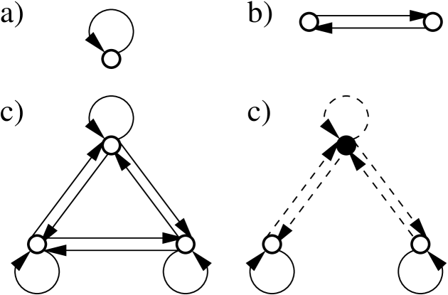
Type-network: In the type-network a node represents a type, an arc is drawn from type $a$ to $b$ if $e_{ab}>0$, and the arc’s weights are given by $e_{ab}$.

Note that since $e_{aa}$ may be nonzero the type-network may contain loops. Fig. 1 shows some simple type-networks. The single-type case is represented by a node with a loop (Fig. 1a). A bipartite population is represented by two nodes with an incoming and an outgoing arc (Fig. 1b). This example could model a heterosexual population with no other distinction than gender or a metapopulation given by people and public places Eubank et al. (2004). A fully mixed population is represented by a complete network (Fig. 1c). A less intuitive example is the type-network shown in Fig. 1d, representing a population divided in two cities and the commuters between them.

II.3 Annealed spanning tree

Given a contact-graph, let us consider an epidemic outbreak starting from a single agent (index case). In the worth case scenario the disease propagates to all the agents that could be reached from the index case using the network connections. Thus, the outbreak is represented by a spanning or causal tree from the index case to all reachable agents. On this tree, the generation of an agent corresponds with the topological or hopping distance from the index case. This picture motivates the introduction of the following branching process:

Definition II.4.

Multi-type Annealed Spanning Tree (AST)

Consider a labeled contact-graph characterized by $\{N_{a},\ p^{(a)}_{k}\}$ and the type-network $\{e_{ab}\}$. The multi-type annealed spanning tree (AST) is the branching process satisfying the following properties:

1. The process start from an index case of type $a\in\{1,\ldots,M\}$ at generation $d=0$. The index case generates $k$ sons with probability distribution $p^{(a)}_{k}$. Each son is of type $b$ with probability $e_{ab}$.

2. Each son at generation $1\leq d<D$ generates $k-1$ sons with probability distribution $q^{(a)}_{k}$. Each son is of type $b$ with probability $e_{ab}$.

3. A son at generation $d=D$ does not generate new sons.

The term annealed means that we are not analyzing the true (quenched) spanning tree on the graph but a branching process with similar statistical properties. This approximation is particularly good if the contact-graph is continuously changing in time albeit the constancy of its statistical properties. A similar mathematical construction has been previously introduced by Newman Newman (2002, 2003). The main difference here is the explicit consideration of the truncation distance $D$. Finally, it is worth noticing that all results derived below are exact for the multi-type AST but an approximation for the original population structure.

III Spreading dynamics

To proceed further we should specify how the disease is transmitted from an agent to its neighbors in the contact-graph. Let $r_{ab}$ be the probability that an infected agent of type $a$ infects a susceptible neighbor of type $b$. Within this work I assume that if $e_{ab}>0$ then $r_{ab}>0$. Indeed, the absence of transmission between two types is taken into account by the corresponding matrix element of $e$. Upon infection we also need to specify when it takes place. Given a type $a$ agent (primary case) and one of its neighbors of type $b$ (secondary case), we define the generation time $X_{ij}^{(a,b)}$ as the time elapse from the infection of the primary case to the infection of the secondary case provided it happens. I assume that the generation times are independent random variables with the distribution function

$$G_{ab}(\tau)={\rm Prob}\left(X_{ij}^{(a,b)}\leq\tau\right)\ ,$$ (10)

parameterized by the type of the primary and secondary cases.

Example III.1 (SIR model).

In the SIR model agents can be in the three exclusive states susceptible, infected and removed. A susceptible agent is one that have not become infected but it is susceptible to acquire the infection. An infected agent is one that have already acquired the disease and can potentially transmit the disease. A removed agent is one that has been previously infected but it is already excluded from the spreading process. Within this work the removal of an agent takes into account intervention strategies resulting in the isolation of infected individuals from the disease transmission chain. The death or “natural” recovery of infected agents was already taken into account during the definition of the contact-graph in subsection II.1.

Consider an agent $i$ of type $a$ and one of its neighbors $j$ of type $b$. Let $Y_{i,j}^{(a,b)}$ be the infection time of agent $j$ by $i$ in the absence of agent’s removal and let $G^{(a,b)}_{\rm I}(\tau)={\rm Prob}\left(Y_{i,j}^{(a,b)}\leq\tau\right)$ be its distribution function. Furthermore, let $Z_{i}^{(a)}$ be the removal time of agent $i$ in the presence of agent’s removal and let $G^{(a,b)}_{\rm R}(\tau)={\rm Prob}\left(Z_{i}^{(a)}\leq\tau\right)$ be its distribution function. The probability that agent $j$ is infected by agent $i$ by time $t$ is given by

$$b_{ab}(t)=\int_{0}^{t}dG_{\rm I}(\tau)\left[1-G_{\rm R}(\tau)\right]\ .$$ (11)

From this magnitude we obtain the probability that agent $j$ gets infected by agent $i$ no matter when

$$r_{ab}=\lim_{t\rightarrow\infty}b_{ab}(t)\ .$$ (12)

and the distribution of generation times

$$G_{ab}(\tau)=\frac{1}{r_{ab}}b_{ab}(\tau)\ .$$ (13)

The SIR model could be further generalized taking immunization into account. In this case non-infected agents are divided into susceptible and immune. If $s_{a}$ is the probability that a type $a$ agent is immune then the probability that agent $j$ is infected by agent $i$ by time $t$ reads

$$b_{ab}(t)=(1-s_{b})\int_{0}^{t}dG_{\rm I}(\tau)\left[1-G_{\rm R}(\tau)\right]\ .$$ (14)

Furthermore, the transmission probability $r_{ab}$ and the generation time distribution $G_{ab}(\tau)$ are obtained substituting this equation into (12) and (13), respectively.

These examples illustrates how to calculate the transmission probability $r_{ab}$ and the generation time distribution $G_{ab}(\tau)$ from the standards models characterizing the spreading of infectious diseases. More important, by encapsulating the model details into $r_{ab}$ and $G_{ab}(\tau)$ we can obtain general results that are independent of these details. Later on, we can analyze the particularities of each model.

III.1 Multi-type age-dependent AST

At this point the local spreading dynamics has been completely specified and we can super-impose it on the multi-type AST.

Definition III.2.

Multi-type age-dependent AST

The multi-type age-dependent AST is composed of two elements, a multi-type AST II.4 and a local spreading dynamics defined by $\{r_{ab},\ G_{ab}(\tau)\}$. The global dynamics is then specified by the following rules

1. The process starts with an infected agent of type $a\in\{1,\ldots,M\}$ while all other agents are susceptible.

2. An infected agent of type $a$ infects each of its neighbors of type $b$ with probability $r_{ab}$ and generation time distribution $G_{ab}(\tau)$.

The age-dependent AST is a generalization of the Bellman-Harris Harris (2002) and Crum-Mode-Jagers Jagers (1975); Mode and Sleeman (2000) multi-type age-dependent branching processes. The key new element is the truncation at a maximum generation, allowing us to consider the small-world property of real networks. In spite of the similarities the mathematical framework I implement deviates substantially from these previous approaches. Indeed, I exploit this truncation making a backward iteration from the final generation $D$ to the index case.

IV Iterative approach

Consider a branch of the AST rooted on a type $a$ agent, at generation $d$, that was infected at time zero. Let $P^{(d,a,b)}_{n}(t)$ be the probability distribution to find $n$ infected type $b$ agents at time $t$ on that branch. In particular $P^{(0,a,b)}_{n}(t)$ is the probability distribution of the total number of infected type $b$ agents at time $t$ on the whole AST, given the index case was of type $a$. Based on the tree structure we can develop an iterative approach to compute $P_{n}^{(d,a,b)}(t)$ recursively.

Lemma IV.1.

Consider a type $a$ infected agent at generation $d$ of the multi-type age-dependent AST. This agent has degree $k$ with probability $p^{(a)}_{k}$ for $d=0$ and excess degree $k-1$ with probability $q^{(a)}_{k}$ for $0<d<D$. Let us index by $\alpha$ its neighbors on the next generation $d+1$, where $\alpha\in\{1,\ldots,k\}$ for $d=0$, $\alpha\in\{1,\ldots,k-1\}$ for $0<d<D$, and $\alpha\in\{\emptyset\}$ for $d=D$. Then

$$\displaystyle P^{(0,a,b)}_{n}(t) = p^{(a)}_{0}\left[\delta_{ab}\delta_{n1}+(1-\delta_{ab})\delta_{n0}\right]$$ (15)

$$+ \sum_{k=1}^{\infty}p^{(a)}_{k}\sum_{n_{1}=0}^{\infty}\dots\sum_{n_{k}=0}^{\infty}\delta_{\sum_{\alpha=1}^{k}n_{\alpha}+\delta_{ab},n}\prod_{\alpha=1}^{k}\sum_{c=1}^{M}e_{ac}$$

$$\times \left[r_{ac}\int_{0}^{t}dG_{ac}(\tau)P^{(1,c,b)}_{n_{\alpha}}(t-\tau)+\delta_{n_{\alpha},0}[1-r_{ac}G_{ac}(t)]\right]$$

$$\displaystyle P^{(d,a,b)}_{n}(t) = q^{(a)}_{1}\left[\delta_{ab}\delta_{n1}+(1-\delta_{ab})\delta_{n0}\right]$$ (16)

$$+ \sum_{k=2}^{\infty}q^{(a)}_{k}\sum_{n_{1}=0}^{\infty}\dots\sum_{n_{k-1}=0}^{\infty}\delta_{\sum_{\alpha=1}^{k-1}n_{\alpha}+\delta_{ab},n}\prod_{\alpha=1}^{k-1}\sum_{c=1}^{M}e_{ac}$$

$$\times \left[r_{ac}\int_{0}^{t}dG_{ac}(\tau)P^{(d+1,c,b)}_{n_{\alpha}}(t-\tau)+\delta_{n_{\alpha},0}[1-r_{ac}G_{ac}(t)]\right]$$

$$P^{(D,a,b)}_{n}(t)=\delta_{ab}\delta_{n1}+(1-\delta_{ab})\delta_{n0}\ .$$ (17)

Proof.

Let $n$ be the number of infected type $b$ agents on a branch rooted at type $a$ agent, and let $n_{\alpha}$ be the infected type $b$ agents on the branches rooted at each of its neighbors $\alpha$. Then

$$n=\delta_{ab}+\sum_{\alpha}n_{\alpha}\ ,$$ (18)

where $\delta_{ab}$ takes into account if the root agent is or it is not of type $b$. The probability distribution of $n$ is given by the sum of all the possible combinations of the random variables $n_{\alpha}$ that satisfy (18). Now, the root agent and its neighbors lie on a tree and therefore $n_{\alpha}$ are independent random variables. Furthermore, all agents at generation $d+1$ has the same statistical properties, i.e. $n_{\alpha}$ are identically distributed random variables. Therefore, the probability of each combination is decomposed into the product of the probability distribution of the number of infected agents of type $b$ on the sub-branches rooted at each neighbor. Thus, taking into account that each neighbors is of type $c$ with probability $e_{ac}$ we obtain

$$P^{(0,a,b)}_{n}(t) = p^{(a)}_{0}\left[\delta_{ab}\delta_{n1}+(1-\delta_{ab})\delta_{n0}\right]$$ (19)

$$+ \sum_{k=1}^{\infty}p^{(a)}_{k}\sum_{n_{1}=0}^{\infty}\dots\sum_{n_{k}=0}^{\infty}\delta_{\sum_{\alpha=1}^{k}n_{\alpha}+\delta_{ab},n}\prod_{\alpha=1}^{k}\sum_{c=1}^{M}e_{ac}Q_{n_{\alpha}}^{(d+1,a,c,b)}(t)\ ,$$

$$P^{(d,a,b)}_{n}(t) = q^{(a)}_{1}\left[\delta_{ab}\delta_{n1}+(1-\delta_{ab})\delta_{n0}\right]$$ (20)

$$+ \sum_{k=2}^{\infty}q^{(a)}_{k}\sum_{n_{1}=0}^{\infty}\dots\sum_{n_{k-1}=0}^{\infty}\delta_{\sum_{\alpha=1}^{k-1}n_{\alpha}+\delta_{ab},n}\prod_{\alpha=1}^{k-1}\sum_{c=1}^{M}e_{ac}Q_{n_{\alpha}}^{(d+1,a,c,b)}(t)\ ,$$

where $Q_{n_{\alpha}}^{(d+1,a,c,b)}(t)$ is the probability distribution of $n_{\alpha}$ which we proceed to calculate.

Let us focus on one neighbor and let us assume that it is of type $c$. With probability $1-r_{ac}$ this agent is not infected at any time and with probability $r_{ac}[1-G_{ac}(t)]$ it is not yet infected at time $t$ given it will be infected at some later time, resulting in

$$Q_{0}^{(d+1,a,c,b)}(t)=1-r_{ac}G_{ac}\ .$$ (21)

On the other hand, with probability $r_{ac}$ the neighbor is infected at some time $\tau$, with distribution function $G_{ac}(\tau)$, and the spreading dynamics continue to subsequent generations. Once the neighbor is infected the number of infected agents of type $b$ on that sub-branch is a random variable with probability distribution $P_{n}^{(d+1,c,b)}(t-\tau)$. Therefore, for $n>0$

$$Q_{n}^{(d+1,a,c,b)}(t)=r_{ac}\int_{0}^{t}dG_{ac}(\tau)P_{n}^{(d+1,c,b)}(t-\tau)\ .$$ (22)

Finally, substituting (21) and (22) into (19) and (20) we obtain equations (15) and (16). The demonstration of (17) is straightforward. For $d=D$ the process stops and therefore there is only one infected agent, the root itself, which is or it is not of type $b$, resulting in (17).

∎

Associated with the probability distribution $P^{(d,a,b)}_{n}(t)$ we introduce that generating function

$$F^{(d,a,b)}(x,t)=\sum_{n=0}^{\infty}P_{n}^{(d,a,b)}(t)x^{n}\ .$$ (23)

Using the recursive relations for the probability distribution (15)-(17) we obtain the following recursive relations for the generating function

$$F^{(0,a,b)}(x,t)=x^{\delta_{ab}}U_{a}\left(\sum_{c=1}^{M}e_{ac}\left[1-r_{ac}G_{ac}(t)+r_{ac}\int_{0}^{t}dG_{ac}(\tau)F^{(1,c,b)}(x,t-\tau)\right]\right)$$ (24)

$$F^{(d,a,b)}(x,t)=x^{\delta_{ab}}V_{a}\left(\sum_{c=1}^{M}e_{ac}\left[1-r_{ac}G_{ac}(t)+r_{ac}\int_{0}^{t}dG_{ac}(\tau)F^{(d,c,b)}(x,t-\tau)\right]\right)$$ (25)

$$F^{(D,a,b)}(x,t)=x^{\delta_{ab}}\ .$$ (26)

These recursive equations are going to be useful in the following calculations.

V Expected behavior

Given a infected agent of type $a$ the expected number of secondary infections of type $b$ it generates is given by

$$R_{ab}=\langle k\rangle_{a}e_{ab}r_{ab}$$ (27)

if it is the index case and by

$$\tilde{R}_{ab}=\langle k\rangle_{a}^{\rm(excess)}e_{ab}r_{ab}$$ (28)

otherwise. The matrices $R$ and $\tilde{R}$ are extensions of the basic reproductive number to the multi-type case. In the following it becomes clear that $\tilde{R}$ is more relevant and therefore I refer to it as the reproductive number matrix.

Lemma V.1.

Consider an ensemble of multi-type age-dependent AST III.2 with index case of type $a$. Let $N_{ab}(t)$ be the mean total number of infected type $b$ agents at time $t$ and let $I_{ab}(t)dt$ be the mean number of type $b$ agents that are infected between time $t$ and $t+dt$. Then

$$N_{ab}(t)=\sum_{d=1}^{D}\left(H\star J^{\star(d-1)}\right)_{ab}(t)\ ,$$ (29)

$$I_{ab}(t)=\sum_{d=1}^{D}\frac{d}{dt}\left(H\star J^{\star(d-1)}\right)_{ab}(t)\ ,$$ (30)

where

$$H_{ab}(t)=R_{ab}G_{ab}(t)\ ,$$ (31)

$$J_{ab}(t)=\tilde{R}_{ab}G_{ab}(t)\ ,$$ (32)

and the multiplication symbolized by $\star$ involves a matrix multiplication and a convolution in time. For instance,

$$\left(H\star J\right)_{ab}(t)=\sum_{c=1}^{M}\int_{0}^{t}d\tau H_{ac}(\tau)J_{cb}(t-\tau)\ .$$ (33)

$$\left(J^{\star 2}\right)_{ab}(t)=\left(J\star J\right)_{ab}(t)\ .$$ (34)

Proof.

Let

$$N^{(d,a,b)}(t)=\frac{\partial F^{(d,a,b)}(1,t)}{\partial x}$$ (35)

be the mean number of infected type $b$ agents on the branch rooted at a type $a$ agent at generation $d$. In particular, $N_{ab}(t)=N^{(0,a,b)}(t)$. Making use of the recursive relations (24)-(26) we obtain

$$N^{(0,a,b)}(t)=\delta_{ab}+\dot{U}_{a}(1)\sum_{c=1}^{M}r_{ac}\int_{0}^{t}dG_{ac}(\tau)N^{(1,c,b)}(t-\tau)$$ (36)

$$N^{(d,a,b)}(t)=\delta_{ab}+\dot{V}_{a}(1)\sum_{c=1}^{M}r_{ac}\int_{0}^{t}dG_{ac}(\tau)N^{(d+1,c,b)}(t-\tau)$$ (37)

$$N^{(D,a,b)}(t)=\delta_{ab}\ .$$ (38)

Iterating these recursive relations from $d=D$ to $d=0$ we obtain (29). Then differentiating with respect to time we finally obtain (30). In this step we also make use of the relation between $\dot{U}(1)$ and $\dot{V}(1)$ and the average degrees (7)-(8).

∎

This Lemma provides explicit equations for the expected progression of an epidemic outbreak. In some particular cases these equations may be further expressed in terms of elementary functions allowing an straightforward interpretation. More generally these equations can be evaluated numerically in cases where further reduction is not possible. In addition, Theorem V.1 is a starting point for calculations addressing some limiting cases, which is the subject of the following subsections.

V.1 Final outbreak size

The final outbreak size is obtained taking the limit $t\rightarrow\infty$ in (29), resulting in

$$N_{ab}(\infty)=\sum_{d=1}^{D}\left(R\tilde{R}^{d-1}\right)_{ab}\ .$$ (39)

When $\tilde{R}$ can be diagonalized we can write $\tilde{R}=PDP^{-1}$, where $P$ is the matrix composed of the eigenvectors of $\tilde{R}$, $D$ is the diagonal matrix constructed from the corresponding eigenvalues ($\rho_{a}$, $a=1,\ldots,M$) and $P^{-1}$ is the inverse of $P$. Thus (39) is reduced to

$$N_{ab}(\infty)=\left(RP\tilde{N}P^{-1}\right)_{ab}\ ,$$ (40)

where $\tilde{N}$ is a diagonal matrix with diagonal entries

$$\tilde{N}_{aa}=\left\{\begin{array}[]{ll}\displaystyle\frac{\rho_{a}^{D}-1}{\rho_{a}-1}\ ,&\mbox{for}\ \rho_{a}\neq 1\\ D\ ,&\mbox{for}\ \rho_{a}=1\end{array}\right.$$ (41)

The following two Theorems show that the only thing we need to estimate the order of magnitude of the expected outbreak size is the largest eigenvalue of the reproductive number matrix $\tilde{R}$.

Theorem V.2 (Complete type-network).

Consider a complete type-network and let $\rho$ be the largest eigenvalue of $\tilde{R}$ (28). Then

$$N_{ab}(\infty)=u_{ab}\frac{\rho^{D}-1}{\rho-1}\ ,$$ (42)

where $u_{ab}$ is indenpendent of $D$.

Proof.

The mixing matrix of a complete type-network is positive defined and, therefore, $R$ (27) and $\tilde{R}$ (28) are positive defined as well. From the Perron-Frobenius Theorem Godsil and Royle (2001) it follows that the largest eigenvalue of $\tilde{R}$ is simple and all the entries of its corresponding left eigenvector $\vec{v}$ are different from zero and have the same sign. In particular we choose all the components of $\vec{v}$ to be positive such that

$$(R\tilde{R}^{d-1})_{ab}=\sum_{c=1}^{M}R_{ac}(\tilde{R}^{d-1})_{cb}=\sum_{c=1}^{M}\frac{R_{ac}}{v_{c}}v_{c}(\tilde{R}^{d-1})_{cb}\ .$$ (43)

Taking into account that $\sum_{c}v_{c}\tilde{R}_{cb}=\rho v_{b}$ we obtain the inequalities

$$u_{ab}^{\rm(min)}\rho^{d-1}\leq(R\tilde{R}^{d-1})_{ab}\leq u_{ab}^{\rm(max)}\rho^{d-1}$$ (44)

where

$$u_{ab}^{\rm(min)}=\min_{c}R_{ac}\frac{v_{b}}{v_{c}}\ ,$$ (45)

$$u_{ab}^{\rm(max)}=\max_{c}R_{ac}\frac{v_{b}}{v_{c}}\ ,$$ (46)

From (42) and (39) we obtain

$$1+u_{ab}^{\rm(min)}\frac{\rho^{D}-1}{\rho-1}\leq N_{ab}(\infty)\leq 1+u_{ab}^{\rm(max)}\frac{\rho^{D}-1}{\rho-1}$$ (47)

Finally, from this equation we obtain (42) with

$$0<u_{ab}^{\rm(min)}\leq u_{ab}\leq u_{ab}^{\rm(max)}<\infty\ ,$$ (48)

where the inequality $u_{ab}>0$ follows from (45).

∎

Figure 2: Strongly connected type-network with six types. The dashed lines indicate the possible paths from type $a$ to $b$. Note that only the types $c$, $c^{\prime}$ and $c^{\prime\prime}$ are neighbors of type $a$ and type $b$ can be only reached from the last two.

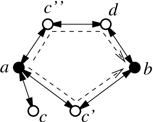
This result can be generalized to type-networks that may not be complete but are still strongly connected, i.e. there is a path from every type $a$ to every type $b$. In this case some entries of $R_{ac}$ and $(\tilde{R}^{d-1})_{cb}$ in (43) may be zero. Intuitively this means that some types $c$ may not be a neighbor of $a$ and, if they are, there may not be a path from $c$ to $b$ (See Fig. 2). More precisely, given a type $a$ let $Out(a)$ be its set of out-neighbors, i.e. $Out(a)=\{c|e_{ac}>0\}$, and given a type $b$ let $In_{d}(b)$ be the set of types from where $b$ is reached after $d$ hops on the type-network, i.e. $In_{d}(b)=\{c|(e^{d})_{cb}>0\}$. Furthermore, let

$$S_{d}^{(a,b)}=Out(a)\cap In_{d-1}(b)$$ (49)

denote the set of types that are out-neighbors of the index case type $a$ and belong to at least one path of length $d$ from $a$ to $b$ on the type-network. For instance, in the example in Fig. 2, $S_{1}^{(a,b)}=\emptyset$, $S_{2}^{(a,b)}=\{c^{\prime}\}$, $S_{3}^{(a,b)}=\{c^{\prime\prime}\}$, and $S_{d}^{(a,b)}\neq\emptyset$ for all $d>3$.

Theorem V.3 (Strongly connected type-network).

Consider a strongly connected type-network. Let $\rho$ be the largest eigenvalue of $\tilde{R}$ (28), $d_{ab}$ the distance on the type-network from type $a$ to $b$, $n=[D/d_{ab}]$ and $D_{ab}=nd_{ab}$. Then

$$N_{ab}(\infty)=u_{ab}\sum_{1\leq d\leq D|S_{d}^{(a,b)}\neq\emptyset}\rho^{d-1}\ ,$$ (50)

where $u_{ab}$ is independent of $D$.

Proof.

The conditions of the Perron-Frobenius theorem Godsil and Royle (2001) are valid beyond positive defined matrices and holds for the mixing matrix representing a strongly connected network. Thus, the largest eigenvalue of $\tilde{R}$ is simple and all the entries of its corresponding eigenvector $\vec{v}$ are different from zero and have the same sign. In particular we choose all the components of $\vec{v}$ to be positive. Based on this fact we can write (43). There may be, however, some entries of $e$ and thus of $R$ (27) and $\tilde{R}^{d-1}$ that are zero. Indeed we can rewrite (43) as

$$(R\tilde{R}^{d-1})_{ab}=\sum_{1\leq c\leq M|c\in S_{d}^{(a,b)}}\frac{R_{ac}}{v_{c}}v_{c}(\tilde{R}^{d-1})_{cb}\ .$$ (51)

Thus $(R\tilde{R}^{d-1})_{ab}=0$ whenever $S_{d}^{(a,b)}=\emptyset$. Otherwise, we obtain the inequalities

$$u_{ab}^{\rm(min)}\rho^{d-1}\leq(R\tilde{R}^{d-1})_{ab}\leq u_{ab}^{\rm(max)}\rho^{d-1}$$ (52)

where

$$u_{ab}^{\rm(min)}=\min_{c\in Out(a)}\frac{v_{b}}{v_{c}}R_{ac}\ ,$$ (53)

$$u_{ab}^{\rm(max)}=\max_{c\in Out(a)}\frac{v_{b}}{v_{c}}R_{ac}\ ,$$ (54)

From (42) and (39) we obtain

$$1+u_{ab}^{\rm(min)}\sum_{1\leq d\leq D|S_{d}^{(a,b)}\neq\emptyset}\rho^{d-1}\leq N_{ab}(\infty)\leq 1+u_{ab}^{\rm(max)}\sum_{1\leq d\leq D|S_{d}^{(a,b)}\neq\emptyset}\rho^{d-1}$$ (55)

From this equation we obtain (50) with

$$0<u_{ab}^{\rm(min)}\leq u_{ab}\leq u_{ab}^{\rm(max)}<\infty\ ,$$ (56)

where the inequality $u_{ab}^{\rm(min)}>0$ follows from (53).

∎

Figure 3: Expexted outbreak size as a function of the largest eigenvalue of the reproductive number matrix for different values of $D$. The region $\rho<1$ is indicated by the dotted pattern.

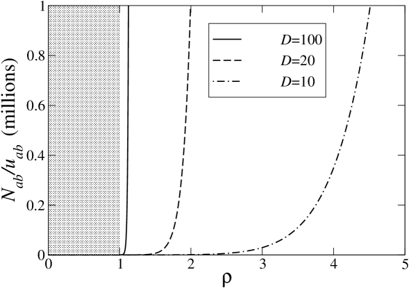
Figure 3 illustrates the predictions of Theorem 42 for complete type-networks. When $\rho<1$ the expected outbreak size is of the order of the prefactor $u_{ab}$ which is not expected to be large. Different behaviors are observed, however, for $\rho>1$ depending on $D$. For $D\gg 1$ there is a dramatic increase in the expected outbreak size. As soon as $\rho>1$ a significant fraction of the agent population becomes affected. In contrast, when $D$ is not so large it becomes clear that the expected outbreak size changes smoothly with increasing $\rho$, including the region around $\rho=1$. This fact becomes relevant when analyzing the impact of intervention strategies (see section V.3). Finally, it is worth mentioning that a similar picture is obtained for the more general case of strongly-connected type-networks, albeit some corrections given by the missing terms the sum in (50).

V.2 Spreading dynamics with constant transmission rate

Now let us consider the particular case where the spreading dynamics is homogeneous, i.e. $G_{ab}(\tau)=G(\tau)$. In this case, from (30) we obtain the incidence

$$I_{ab}(t)=\sum_{d=1}^{D}\left(R\tilde{R}^{d-1}\right)_{ab}G^{\star d}(t)\ .$$ (57)

In particular when $\tilde{R}$ can be diagonalized we rewrite (57) as

$$I_{ab}(t)=\left(RP\tilde{I}(t)P^{-1}\right)_{ab}\ ,$$ (58)

where $\tilde{I}(t)$ is a time dependent diagonal matrix with diagonal entries

$$\tilde{I}_{aa}(t)=\sum_{d=1}^{D}G^{\star d}(t)\ .$$ (59)

Example V.4.

Consider the case $M=2$ with the reproductive number matrices

$$R=\left[\begin{matrix}k_{1}&k_{2}\\ k_{2}&k_{1}\\ \end{matrix}\right]\ ,\ \ \ \ \tilde{R}=\left[\begin{matrix}K_{1}&K_{2}\\ K_{2}&K_{1}\\ \end{matrix}\right]$$ (60)

Since $\tilde{R}$ is symmetric it can be diagonalized and $P^{-1}=P^{\rm T}$, where $P^{\rm T}$ is the transpose of $P$. In this case $\tilde{R}=PDP^{\rm T}$ with

$$D=\left[\begin{matrix}\rho_{1}&0\\ 0&\rho_{2}\\ \end{matrix}\right]\ ,\ \ \ \ P=\frac{1}{\sqrt{2}}\left[\begin{matrix}1&1\\ 1&-1\\ \end{matrix}\right]$$ (61)

where

$$\rho=\rho_{1}=K_{1}+K_{2}\ ,\ \ \ \ \rho_{2}=K_{1}-K_{2}$$ (62)

are the eigenvalues of $\tilde{R}$. Assuming an index case is of type $a=1$ from (58) we finally obtain

$$I_{11}(t)=\frac{k_{1}+k_{2}}{2}\tilde{I}_{11}(t)+\frac{k_{1}-k_{2}}{2}\tilde{I}_{22}(t)$$ (63)

$$I_{12}(t)=\frac{k_{1}+k_{2}}{2}\tilde{I}_{11}(t)-\frac{k_{1}-k_{2}}{2}\tilde{I}_{22}(t)\ ,$$ (64)

This example shows that in some cases we can exactly calculate the expected progression of an epidemic outbreak. More generally we obtain the following asymptotic behaviors.

Theorem V.5.

Consider a strongly connected type network and a homogeneous and exponential distribution of generation times $G_{ab}=1-e^{-\lambda\tau}$, where $\lambda$ is the transmission rate. Let $\rho$ be the largest eigenvalue of $\tilde{R}$ (28) and let

$$\theta=\frac{D-1}{\rho}\ .$$ (65)

$\theta\gg 1$: If $\rho>1$ and $1\ll\lambda t\ll\theta$ then

$$I_{ab}(t)\sim e^{(\rho-1)\lambda t}\ .$$ (66)

$\theta\ll 1$: If $\lambda t\gg\theta$ then

$$\frac{I_{ab}(t)}{N_{ab}(\infty)}=\frac{\lambda(\lambda t)^{D_{ab}-1}e^{-\lambda t}}{(D_{ab}-1)!}\left[1+{\cal O}\left(\frac{\theta}{\lambda t}\right)\right]\ ,$$ (67)

where $D_{ab}$ is the same as in Theorem V.3.

Proof.

$\theta\gg 1$: Following the same guidelines of the Theorem V.3 proof we arrive to the inequality

$$u_{ab}^{\rm(min)}f_{ab}(t)\leq I_{ab}(t)\leq u_{ab}^{\rm(max)}f_{ab}(t)\ ,$$ (68)

where

$$f_{ab}(t)=\sum_{1\leq d\leq D|S_{d}^{(a,b)}\neq\emptyset}\frac{\lambda(\rho\lambda t)^{d-1}e^{-\lambda t}}{(d-1)!}$$ (69)

The Laplace transform of $f_{ab}(t)$ is given by

$$\hat{f}_{ab}(\omega)=\int_{0}^{\infty}dtf_{ab}(t)e^{-\omega t}=\frac{a}{\rho}\sum_{1\leq d\leq D|S_{d}^{(a,b)}\neq\emptyset}\left(\frac{\rho\lambda}{\omega+\lambda}\right)^{d}\ .$$ (70)

When $D\rightarrow\infty$ this series converges only for $\omega>(\rho-1)\lambda$. Therefore, $f_{ab}(t)\sim e^{(\rho-1)\lambda t}$ when $\lambda t\rightarrow\infty$.

$\theta\ll 1$: The demonstration of this case is straightforward. From Theorem V.3 it follows that $(R\tilde{R}^{d-1})_{ab}$ is of order $\rho^{d-1}$ for $S_{d}^{(a,b)}\neq\emptyset$. Therefore, for $\rho\gg D$ the sum in (57) is dominated by the $d=D_{ab}$ term. Corrections are given by the ratio between the $d=D_{ab}$ and the preceeding term satisfying $S_{d}^{(a,b)}\neq\emptyset$, which is at most $d=D_{ab}-1$.

∎

The case $\theta\gg 1$ provides the connection between this work and multi-type age-dependent branching processes with an infinite number of generations. Indeed, Mode have already demonstrated the exponential growth regime for the case $D=\infty$ (see Mode (1971), Chapter 3). Theorem V.5 shows that on the other limit $\theta\ll 1$ the spreading dynamics is instead characterized by a gamma distribution, which is also the case for the single-type caseVazquez (2006a, b, ).

Figure 4: (a) Schematic representation of the evolution of a disease within an agent, starting from the moment the agent gets infected, passing through a latent state where the agent is not infectious and finally becoming infectious. (b) Gamma probability density function $g(\tau)=\dot{G}(\tau)$ for different values of $\alpha$. (c) Number of secondary cases generated by a primary case for a SARS outbreak in Singapore, as reported in Lipsitch and et al (2003) (bars). The solid line is the best fit to the gamma probability density function times a pre-factor, resulting in $\alpha\approx 4.3$. (d) Plot of the parameter $\theta(\alpha)$ dividing the exponential and power law initial growth regimes as a function of the number of intermediary steps.

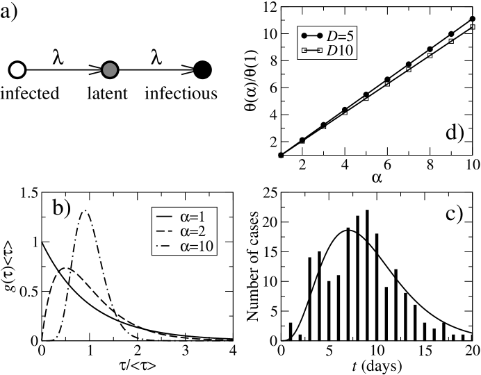
Theorem V.5 can be extended to consider other generation time distributions, such as a gamma distribution

$$G(\tau)=\frac{1}{\Gamma(\alpha)}\int_{0}^{\lambda t}dxx^{\alpha-1}e^{-x}\ ,$$ (71)

where $\alpha\geq 1$. The gamma distribution can be interpreted as the existence of $\alpha-1$ intermediary steps before an agent becomes infectious (see Fig. 4a,b). For $\alpha=1$ we recover the exponential distribution which corresponds with the absence of intermediary steps. The gamma distribution can be also obtained from the fit to some empirical distribution of generation times (see Fig. 4c).

In this case there are two important modifications to Theorem V.5. First, the parameter $\theta$ is now given by

$$\theta(\alpha)=\frac{[(\alpha D-1)\cdots(\alpha D-\alpha)]^{\frac{1}{\alpha}}}{\rho}\ ,$$ (72)

which increases approximately linearly with increasing $\alpha$ (see Fig. 4d). Second, in the regime $\theta(\alpha)\gg 1$ although the fraction of infected agents is still given by a gamma distribution the exponent of the initial power law growth is given by $\alpha D$, i.e.

$$\frac{I_{ab}(t)}{N_{ab}(\infty)}\approx\frac{\lambda(\lambda t)^{\alpha D_{ab}-1}e^{-\lambda t}}{\Gamma(\alpha D_{ab}-1)}\ .$$ (73)

Therefore, the existence of intermediary steps reduces the the small-world effect by a factor given by the number of intermediary steps $\alpha$. For instance, by a factor of about four for SARS (Fig. 4b).

V.3 Impact of intervention strategies

The expected outbreak size is a monotonic increasing function of $\rho$ (50), which plays the role of the basic reproductive number in homogeneous populations Anderson and May (1991); Fraser et al. (2004). Therefore, the aim of intervention strategies is to reduce the characteristic reproductive number $\rho$. On the other hand, intervention strategies implies an economical cost, including but not limited to the development of new vaccines and their deployment through vaccination campaigns. Our task is to design optimal intervention strategies that minimize the expected outbreak size with a feasible economical cost.

To be more precise let us consider a scenario where the disease is transmitted at constant rate $\lambda$ from infected to susceptible agents, infected agents are isolated at a rate $\mu$ and a fraction $s$ of the population is immune to the disease. In this case the infection and removal times follows the exponential distribution functions $G_{\rm I}(\tau)=1-e^{-\lambda\tau}$ and $G_{\rm R}(\tau)=1-e^{-\mu\tau}$, respectively. Thus, from (12) we obtain $r_{ab}=1-\beta$ where

$$\beta=1-\frac{\lambda}{\lambda+\mu}(1-s)\ ,$$ (74)

is the blocking fraction, i.e. the fraction of potential disease transmissions that are blocked either because of immunization or patient isolation. Since $r_{ab}=1-\beta$ is independent of the primary and secondary case types we can write the reproductive number matrices (27) and (28) as $R_{ab}=(1-\beta)K$ and $\tilde{R}=(1-\beta)\tilde{K}$, respectively, where

$$K_{ab}=\langle k\rangle_{a}e_{ab}\ ,\ \ \ \ \tilde{K}_{ab}=\langle k\rangle_{a}^{(\rm excess)}e_{ab}\ .$$ (75)

In turn, the largest eigenvalue of $\tilde{R}$ is given by

$$\rho=(1-\beta)\kappa\ ,$$ (76)

where $\kappa$ is the largest eigenvalue of $\tilde{K}$.

From the analysis made in section V.1 it follows that there are two different scenarios depending $D_{ab}$. For simplicity let us focus on the complete type-network case where $D_{ab}=D$. When $D\gg 1$ the target of intervention strategies is $\rho=1$, which is the consensus in the literature Anderson and May (1991); Fraser et al. (2004). The blocking fraction to achieve this is obtained from (76), resulting in

$$\beta_{c}=1-\frac{1}{\kappa}\ .$$ (77)

This result has been already reported, at least for the case of two types Anderson and May (1991). When $D$ is small, however, the expected outbreak size is a smooth function of $\rho$ (see Fig. 3). Therefore, $\beta_{c}$ does not represent a threshold value in small-world populations.

So far we have considered homogenous intervention strategies. Now let us assume that the rate of patient isolation and the immunized fraction are now different for each agent’s type and given by $\mu_{a}$ and $s_{a}$, respectively. In this case the blocking fraction is given by

$$\beta_{ab}=1-\frac{\lambda}{\lambda+\mu_{a}}(1-s_{b})\ ,$$ (78)

and $r_{ab}=1-\beta_{ab}$, which depends on the type of both the primary and secondary case. From the Perron-Frobenius Theorem it follows that $\rho$ is a continuous increasing function of all the entries of the corresponding matrix $\tilde{R}$ Gantmacher (1990). Since $\tilde{R}_{ab}=(1-\beta_{ab})\tilde{K}_{ab}$ then $\rho$ is a continuous decreasing function of $\theta_{ab}$ for all $(a,b)$. The goal is to determine which strategy leads to the largest reduction of $\rho$.

Example V.6.

Consider the spread of HIV on an heterosexual population with no further distinction beyond gender. In this case the type-network is bipartite (see Fig. 1b). Let $k_{1}$ and $k_{2}$ be the average excess degree for the connections from women to men and biceversa. Let also assume that the rate of patient isolation is zero and that we could immunize a fraction $s$ of the overall population, distributed between a fraction $xs$ and $(1-x)s$ of immunized women and men, respectively. The question is to determine the value of $x$ representing the best intervention strategy. In this case the reproductive number matrix is given by

$$\tilde{R}=\left[\begin{matrix}0&[1-(1-x)s]k_{2}\\ (1-xs)k_{1}&0\end{matrix}\right]$$ (79)

and it has the largest eigenvalue

$$\rho=\sqrt{[1-s+x(1-x)s^{2}]k_{1}k_{2}}\ .$$ (80)

It results that $\rho$ is minimum for $x=0$ or $x=1$, i.e. the best intervention strategy is to direct all the immunization resources to only one of the sub-populations.

VI Discussion

There is significant evidence that social networks are characterized by (i) wide connectivity fluctuations and (ii) the small-world property Watts and Strogatz (1998). The variability in the number of contacts (i) has a direct impact on the reproductive number. This fact has been taken into account since the seminal works of May and Anderson considering the variability in the rate of sexual partner acquisitionMay and Anderson (1987, 1988); Anderson and May (1991). More recently it has gained attention for other infectious diseases as well, following the observation of super-spreading events in the 2002-2003 SARS epidemics Anderson and et al (2004); Galvani and May (2005); Lloyd-Smith et al. (2005). Yet, the small-world property (ii) has been completely neglected.

From my studies of the single type case Vazquez (2006a, b, ) I have shown that intervention strategies are modulated by the average distance $D$ between agents in the corresponding contact-graph. In this work I have demonstrated that this result is also valid for heterogeneous populations. In this last case the characteristic reproductive number is given by the largest eigenvalue of the reproductive number matrix. The good news is that in spite of this modulation by $D$ the target of intervention strategies is still the characteristic reproductive number. That is, the expected outbreak size still decreases with decreasing the characteristic reproductive number. The bad news is that to quantify the impact of the intervention strategies we need to estimate $D$.

There are different paths to estimate $D$. First, we can use a direct approach as the Milgram’s experiments Milgram (1967). Second, we can measure other network properties such as the degree distribution and then try to estimate $D$ using network models Bollobás (2001); Chung and Lu (2002); Bollobás and Riordan (2003); Cohen and Havlin (2003); Vazquez (2003); J. Leskovec and Faloutsos . Finally, I have shown that the progression of the expected number of new infections is modulated by $D$ (see Vazquez (2006a, b, ) and section III). More precissely, in small world populations the incidence is expected to grow as a power law and we can estimate $D$ from the power law exponent.

Further work is required to test the validity of the coarse grained description of the type-network approach. This can be done by running agent based simulations where we can have a strict control of the different statistical properties characterizing the population structure. These statistical properties can be then plug in into the type network approach to obtain qualitative and quantitative predictions that can be compared with the simulations results.

In conclusion, this work opens new avenues to future research on the spreading of infectious diseases on heterogeneous populations. It allows for a qualitative understanding through the analysis of the type-network representation of the mixing matrix. More important, it leads to general results that can be tackled case by case using exact or approximate calculations and numerical computations.

This work was supported by NSF Grants No. ITR 0426737 and No. ACT/SGER 0441089.

References

- Anderson and May (1991) R. M. Anderson and R. M. May, Infectious diseases of humans (Oxford Univ. Press, New York, 1991).
- Hufnagel et al. (2004) L. Hufnagel, D. Brockmann, and G. T, Proc. Natl. Acad. Sci. USA 101, 15124 (2004).
- Koopman (2004) J. Koopman, Annu. Rev. Public Health 25, 303 (2004).
- Germann et al. (2006) T. C. Germann, K. Kadau, I. M. Longini, and C. A. Macken, Proc. Natl. Acad. Sci. USA 103, 5935 (2006).
- Colizza et al. (2006) V. Colizza, A. Barrat, M. Barthelemy, and A. Vespignani, Proc. Natl. Acad. Sci. USA 103, 2015 (2006).
- May and Anderson (1987) R. M. May and R. M. Anderson, Nature 326, 137 (1987).
- Anderson and et al (2004) R. M. Anderson and et al, Phil. Trans. R. Soc. Lond. B 359, 1091 (2004).
- Lloyd-Smith et al. (2005) J. O. Lloyd-Smith, S. J. Schreiber, P. E. Kopp, and W. M. Getz, Nature 438, 355 (2005).
- May and Anderson (1988) T. M. May and R. M. Anderson, Phil. Trans. R. Soc. Lond. B 321, 565 (1988).
- Liljeros et al. (2001) F. Liljeros, C. R. Edling, L. A. N. Amaral, H. E. Stanley, and Y. Berg, Nature 411, 907 (2001).
- Jones and Handcock (2003) J. H. Jones and M. S. Handcock, Proc. R. Soc. Lond. B Biol. Sci. 270, 1123 (2003).
- Schneeberger et al. (2004) A. Schneeberger, C. H. Mercer, S. A. Gregson, N. M. Fergurson, C. A. Nyamukapa, R. M. Anderson, A. M. Johnson, and G. P. Garnett, Sex. Transm. Dis. 31, 380 (2004).
- Pastor-Satorras and Vespignani (2001) R. Pastor-Satorras and A. Vespignani, Phys. Rev. Lett. 86, 3200 (2001).
- Moore and Newman (2000) C. Moore and M. E. J. Newman, Phys. Rev. E 61, 5678 (2000).
- Albert and Barabási (2001) R. Albert and A.-L. Barabási, Rev. Mod. Phys. 74, 47 (2001).
- Rvachev and Longini (1985) L. A. Rvachev and I. M. Longini, Math. Biosci. 75, 3 (1985).
- Flahault et al. (1988) A. Flahault, S. Letrait, P. Blin, S. Hazout, J. Menares, and A. J. Valleron, Stat. Med. 7, 1147 (1988).
- Eubank et al. (2004) S. Eubank, H. Guclu, V. S. A. Kumar, M. Marathe, A. Srinivasan, Z. Toroczcai, and N. Wang, Nature 429, 180 (2004).
- Newman (2003) M. E. J. Newman, Phys. Rev. E 67, 026126 (2003).
- Mode (1971) C. J. Mode, Multitype branching processes (Elsevier, New York, 1971).
- Vazquez (2006a) A. Vazquez, in AMS-DIMACS Volume on Discrete Methods in Epidemiology (AMS, in press, 2006a).
- Vazquez (2006b) A. Vazquez, Phys. Rev. Lett. 96, 038702 (2006b).
- (23) A. Vazquez, http://arxiv.org/q-bio.PE/0603010.
- Friedman and et al (1997) S. R. Friedman and et al, Am. J. Pub. Health 87, 1289 (1997).
- Edmunds et al. (1997) W. J. Edmunds, C. J. O. O’Callaghan, and D. J. Nokes, Proc. R. Soc. Lond. B 264, 949 (1997).
- Ghani and Garnett (1998) A. C. Ghani and G. P. Garnett, J. R. Statist. Soc. A 161, 227 (1998).
- Keeling and Eames (2005) M. J. Keeling and K. T. D. Eames, J. R. Soc. Interface 2, 297 (2005).
- Watts and May (1992) C. H. Watts and R. M. May, Math. Biosci. 108, 89 (1992).
- Kretzschmar and Morris (1996) M. Kretzschmar and M. Morris, Math. Biosci. 133, 165 (1996).
- Garnett and A. M (1997) G. P. Garnett and J. A. M, AIDS 11, 681 (1997).
- Watts (1999) D. J. Watts, Small Worlds: The Dynamics of Networks between Order and Randomness (Princeton University Press, Princeton, New Jersey, 1999).
- Milgram (1967) S. Milgram, Psychology today 2, 60 (1967).
- Watts and Strogatz (1998) D. J. Watts and S. H. Strogatz, Nature 393, 440 (1998).
- Bollobás (2001) B. Bollobás, Random Graphs (Cambridge: Cambridge University Press, 2001).
- Chung and Lu (2002) F. Chung and L. Lu, Proc. Natl. Acad. Sci. USA 99, 15879 (2002).
- Bollobás and Riordan (2003) B. Bollobás and O. M. Riordan, in Handbook of Graphs and Networks: From the Genome to the Internet, edited by S. Bornholdt and H. G. Schuster (Wiley-VCH, Weinheim, 2003), pp. 1–34.
- Cohen and Havlin (2003) R. Cohen and S. Havlin, Phys. Rev. Lett. 90, 058701 (2003).
- (38) J. K. J. Leskovec and C. Faloutsos, http://arxiv.org/physics/0603229.
- Newman (2002) M. E. J. Newman, Phys. Rev. Lett. 89, 208701 (2002).
- Harris (2002) T. E. Harris, The Theory of Branching Processes (Springer-Verlag, Berlin, 2002).
- Jagers (1975) P. Jagers, Branching processes with biological applications (Wiley, London, 1975).
- Mode and Sleeman (2000) C. J. Mode and C. K. Sleeman, Stochastic processes in epidemiology (World Scientific, Singapore, 2000).
- Godsil and Royle (2001) C. Godsil and G. Royle, Algebraic graph theory (Springer, New York, 2001).
- Lipsitch and et al (2003) M. Lipsitch and et al, Science 300, 1966 (2003).
- Fraser et al. (2004) C. Fraser, S. Riley, R. Anderson, and N. M. Ferguson, Proc. Natl. Acad. Sci. USA 101, 6146 (2004).
- Gantmacher (1990) F. R. Gantmacher, Mathrix Theory (AMS, 1990), vol. I.
- Galvani and May (2005) A. P. Galvani and R. M. May, Nature 438, 293 (2005).
- Vazquez (2003) A. Vazquez, Phys. Rev. E 67, 056104 (2003).