Methods of robustness analysis for Boolean models
of gene control networks

Abstract

As a discrete approach to genetic regulatory networks, Boolean models provide an essential qualitative description of the structure of interactions among genes and proteins. Boolean models generally assume only two possible states (expressed or not expressed) for each gene or protein in the network as well as a high level of synchronization among the various regulatory processes.

In this paper, we discuss and compare two possible methods of adapting qualitative models to incorporate the continuous-time character of regulatory networks. The first method consists of introducing asynchronous updates in the Boolean model. In the second method, we adopt the approach introduced by L. Glass to obtain a set of piecewise linear differential equations which continuously describe the states of each gene or protein in the network.

We apply both methods to a particular example: a Boolean model of the segment polarity gene network of Drosophila melanogaster. We analyze the dynamics of the model, and provide a theoretical characterization of the model’s gene pattern prediction as a function of the timescales of the various processes.

1 Introduction

Genes and gene products interact on several levels. At the genomic level, transcription factors can activate or inhibit the transcription of genes to give mRNAs. Since these transcription factors are themselves products of genes, the ultimate effect is that genes regulate each other’s expression as part of gene regulatory networks. Similarly, proteins can participate in diverse post-translational interactions that lead to modified protein functions or to formation of protein complexes that have new roles; the totality of these processes is called a protein-protein interaction network. In many cases different levels of interactions are integrated - for example, when the presence of an external signal triggers a cascade of interactions that involves biochemical reactions, protein-protein interactions and transcriptional regulation.

During the last decade, genomics, transcriptomics and proteomics have produced an incredible quantity of molecular interaction data, contributing to genome-scale maps of protein interaction networks [1, 2, 3] and transcriptional regulatory networks [4]. Network analysis of these maps revealed intriguing topological similarities [5]. At the same time, it has been increasingly realized that cellular interaction maps only represent a network of possibilities, and not all edges are present and active in vivo in a given condition or in a given cellular location [2, 6]. Therefore, only an integration of (time-dependent) interaction and activity information will be able to give the correct dynamical picture of a cellular network.

For many biological networks, and in particular genetic control or regulatory networks, detailed information on the kinetic rates of protein-protein or protein-DNA interactions is rarely available. However, for many biological systems, evidence shows that regulatory relationships can be sigmoidal and be well approximated by step functions. In this case, Boolean models, where every variable has only two states (ON/OFF), and the dynamics is given by a set of logical rules, are frequently appropriate descriptions of the network of interactions among genes and proteins. Examples include models of genetic networks in the fruit fly Drosophila melanogaster [7, 8] and the flowering plant Arabidopsis thaliana [9, 10].

While Boolean models introduce biologically unrealistic time constraints (typically, such models use synchronous updates, which inherently assume that the various biological processes have the same duration), they still provide significant qualitative information on the underlying structure of the network. On the other hand, continuous models certainly have a more realistic time description of a biological system. But, in the absence of information on the kinetic rates, continuous models include many unknown parameters, and analysis of the system involves exploring the (often large) state space of parameters. An important (continuous) model for Drosophila melanogaster segment polarity genes was first developed in [11], where a thorough investigation of the parameter space showed that the system is very robust with respect to variations in the kinetic constants. Both this continuous model and the discrete model [8] agree in their overall conclusions regarding the robustness of the segment polarity gene network.

In this paper, we propose two new approaches to the analysis of Boolean models, which combine discrete logical rules and structure with more realistic assumptions regarding the relative timescales of the genetic processes. The first method introduces asynchronous updates in the Boolean model; since update times are randomly chosen, the model is now stochastic (see also [12]). The second method associates to the discrete variables a set of continuous variables, whose dynamics is given by a piecewise linear system of differential equations, thus introducing a simple “hybrid” model in the manner first suggested by L. Glass and collaborators in [13, 14, 15]. These methods allow us to naturally probe the system with respect to perturbations in the time dynamics to analyze its performance. Both methods uncover the robustness of the segment polarity gene model [8], and its ability to correctly predict the final gene expression pattern.

Section 2 summarizes the Boolean model [8], to be analyzed with our methods. The asynchronous updates and the Glass-type methods are described and applied in Sections 3 and 4, respectively. In Section 5, we discuss the effects of perturbations in initial gene expression, and the development of mutant phenotypes. Finally, in Section 6 we show that under a timescale separation between posttranslational and translational processes in the model [8], we are able to analytically and exactly compute how frequently the model will predict the correct gene pattern.

2 The segment polarity gene network in Drosophila

We will apply our analysis to a Boolean model of the interactions among the Drosophila melanogaster segment polarity genes. This gene network represents the last step in the hierarchical cascade of gene families initiating the segmented body of the fruit fly. While genes in preceding stages of development act transiently, the segment polarity genes are expressed throughout the life of the fly. The best characterized segment polarity genes include engrailed (en), wingless (wg), hedgehog (hh), patched (ptc), cubitus interruptus (ci) and sloppy paired ($slp$), coding for the corresponding proteins, which we will represent by capital letters (EN, WG, HH, PTC, CI and SLP). Two additional proteins, resulting from transformations of the protein CI, also play important roles: CI may be converted into a transcriptional activator, CIA, or may be cleaved to form a transcriptional repressor CIR.

The expression pattern of the Drosophila segment polarity genes (see Table 2) is maintained almost unmodified for three hours, during which time the embryo is divided into $14$ parasegments. Each of these parasegments is composed of about 4 cells, delimited by furrows positioned between the wg and en -expressing cells [16].

The Boolean model that we will study was introduced and developed by one of us in [8]. (Further robustness analysis was also developed in [12].) In this model, a parasegment of four cells is considered: the variables are the expression levels of the segment polarity genes and proteins (listed above) in each of the four cells (the total number of nodes in the network is thus $4\times 13=52$.). The expression level of each gene or protein is assumed to be either 0 (OFF) or 1 (ON). The model successfully describes the transition from the initial expression pattern (1) to a final pattern two or three developmental stages later, when the embryo has been clearly divided into parasegments (see first entry of Table 2). As discussed in [8], the evolution of these gene expression patterns is well described by a set of logical rules, which are depicted in Table 1.

We adopt the notation “$\mbox{\it wg}_{1}^{k}$” or “$\mbox{\it wg}_{1}(k)$” to represent the state of wingless mRNA in the first cell of the parasegment at time $k$. Similar notations apply for other mRNAs and proteins. Periodic boundary conditions are assumed, meaning that: $node_{4+1}=node_{1}$ and $node_{1-1}=node_{4}$. The wild type initial pattern corresponds to:

$$\mbox{\it wg}_{4}^{0}=1,\ \mbox{\it en}_{1}^{0}=1,\ \mbox{\it hh}_{1}^{0}=1,\ \mbox{\it ptc}_{2,3,4}^{0}=1,\ \mbox{\it ci}_{2,3,4}^{0}=1,$$ (1)

with the remaining nodes zero.

Table 1: Regulatory functions governing the states of segment polarity gene products in the model. Each node is labeled by its biochemical symbol and subscripts signify cell number.

Node	Boolean updating function (synchronous algorithm)
$\mbox{\it SLP}_{i}$	$\mbox{\it SLP}_{i}(k+1)=\left\{\begin{array}[]{lllll}0&\mbox{if}&i\in\{1,2\}\\ 1&\mbox{if}&i\in\{3,4\}\\ \end{array}\right.$
$\mbox{\it wg}_{i}$	$\mbox{\it wg}_{i}(k+1)=(\mbox{\it CIA}_{i}(k)$ and $\mbox{\it SLP}_{i}(k)$ and not $\mbox{\it CIR}_{i}(k))$
	or $[\mbox{\it wg}_{i}(k)$ and $(\mbox{\it CIA}_{i}(k)$ or $\mbox{\it SLP}_{i}(k))$ and not $\mbox{\it CIR}_{i}(k)]$
$\mbox{\it WG}_{i}$	$\mbox{\it WG}_{i}(k+1)=\mbox{\it wg}_{i}(k)$
$\mbox{\it en}_{i}$	$\mbox{\it en}_{i}(k+1)=(\mbox{\it WG}_{i-1}(k)$ or $\mbox{\it WG}_{i+1}(k))$ and not $\mbox{\it SLP}_{i}(k)$
$\mbox{\it EN}_{i}$	$\mbox{\it EN}_{i}(k+1)=\mbox{\it en}_{i}(k)$
$\mbox{\it hh}_{i}$	$\mbox{\it hh}_{i}(k+1)=\mbox{\it EN}_{i}(k)$ and not $\mbox{\it CIR}_{i}(k)$
$\mbox{\it HH}_{i}$	$\mbox{\it HH}_{i}(k+1)=\mbox{\it hh}_{i}(k)$
$\mbox{\it ptc}_{i}$	$\mbox{\it ptc}_{i}(k+1)=\mbox{\it CIA}_{i}(k)$ and not $\mbox{\it EN}_{i}(k)$ and not $\mbox{\it CIR}_{i}(k)$
$\mbox{\it PTC}_{i}$	$\mbox{\it PTC}_{i}(k+1)=\mbox{\it ptc}_{i}(k)$ or $(\mbox{\it PTC}_{i}(k)$ and not $\mbox{\it HH}_{i-1}(k)$
	and not $\mbox{\it HH}_{i+1}(k))$
$\mbox{\it ci}_{i}$	$\mbox{\it ci}_{i}(k+1)=$ not $\mbox{\it EN}_{i}(k)$
$\mbox{\it CI}_{i}$	$\mbox{\it CI}_{i}(k+1)=ci_{i}(k)$
$\mbox{\it CIA}_{i}$	$\mbox{\it CIA}_{i}(k+1)=CI_{i}(k)$ and [not $\mbox{\it PTC}_{i}(k)$ or $\mbox{\it HH}_{i-1}(k)$
	or $\mbox{\it HH}_{i+1}(k)$ or $\mbox{\it hh}_{i-1}(k)$ or $\mbox{\it hh}_{i+1}(k)$]
$\mbox{\it CIR}_{i}$	$\mbox{\it CIR}_{i}(k+1)=\mbox{\it CI}_{i}(k)$ and $\mbox{\it PTC}_{i}(k)$ and not $\mbox{\it HH}_{i-1}(k)$
	and not $\mbox{\it HH}_{i+1}(k)$ and not $\mbox{\it hh}_{i-1}(k)$ and not $\mbox{\it hh}_{i+1}(k)$

2.1 Steady states of the Boolean model

A complete analysis of the steady states is found in [8]. Table 2 summarizes these results, indicating the expressed nodes in each of the six steady-states. We note that three of the four main steady states agree perfectly with experimentally observed states corresponding to wild type, to ptc knockout mutant (broad striped) and to en, wg or hh knockout mutant (non-segmented) embryonic patterns ([17, 18]; see [8] for more references).

Table 2: Complete characterization of the model’s steady states.

Steady state	Expressed nodes
wild type	$\mbox{\it wg}_{4}$, $\mbox{\it WG}_{4}$, $\mbox{\it en}_{1}$, $\mbox{\it EN}_{1}$, $\mbox{\it hh}_{1}$, $\mbox{\it HH}_{1}$,
	$\mbox{\it ptc}_{2,4}$, $\mbox{\it PTC}_{2,3,4}$, $\mbox{\it ci}_{2,3,4}$,
	$\mbox{\it CI}_{2,3,4}$, $\mbox{\it CIA}_{2,4}$, $\mbox{\it CIR}_{3}$
broad stripes	$\mbox{\it wg}_{3,4}$, $\mbox{\it WG}_{3,4}$, $\mbox{\it en}_{1,2}$, $\mbox{\it EN}_{1,2}$, $\mbox{\it hh}_{1,2}$, $\mbox{\it HH}_{1,2}$,
	$\mbox{\it ptc}_{3,4}$, $\mbox{\it PTC}_{3,4}$, $\mbox{\it ci}_{3,4}$, $\mbox{\it CI}_{3,4}$, $\mbox{\it CIA}_{3,4}$
no segmentation	$\mbox{\it ci}_{1,2,3,4}$, $\mbox{\it CI}_{1,2,3,4}$, $\mbox{\it PTC}_{1,2,3,4}$, $\mbox{\it CIR}_{1,2,3,4}$
wild type variant	$\mbox{\it wg}_{4}$, $\mbox{\it WG}_{4}$, $\mbox{\it en}_{1}$, $\mbox{\it EN}_{1}$, $\mbox{\it hh}_{1}$, $\mbox{\it HH}_{1}$,
	$\mbox{\it ptc}_{2,4}$, $\mbox{\it PTC}_{1,2,3,4}$, $\mbox{\it ci}_{2,3,4}$,
	$\mbox{\it CI}_{2,3,4}$, $\mbox{\it CIA}_{2,4}$, $\mbox{\it CIR}_{3}$
ectopic	$\mbox{\it wg}_{3}$, $\mbox{\it WG}_{3}$, $\mbox{\it en}_{2}$, $\mbox{\it EN}_{2}$, $\mbox{\it hh}_{2}$, $\mbox{\it HH}_{2}$,
	$\mbox{\it ptc}_{1,3}$, $\mbox{\it PTC}_{1,3,4}$, $\mbox{\it ci}_{1,3,4}$,
	$\mbox{\it CI}_{1,3,4}$, $\mbox{\it CIA}_{1,3}$, $\mbox{\it CIR}_{4}$
ectopic variant	$\mbox{\it wg}_{3}$, $\mbox{\it WG}_{3}$, $\mbox{\it en}_{2}$, $\mbox{\it EN}_{2}$, $\mbox{\it hh}_{2}$, $\mbox{\it HH}_{2}$,
	$\mbox{\it ptc}_{1,3}$, $\mbox{\it PTC}_{1,2,3,4}$, $\mbox{\it ci}_{1,3,4}$,
	$\mbox{\it CI}_{1,3,4}$, $\mbox{\it CIA}_{1,3}$, $\mbox{\it CIR}_{4}$

2.2 The regulatory function of the sloppy paired gene

The rule for SLP protein in Table 1 summarizes in a simple way the experimental observations on the expression and regulatory activity of the sloppy paired gene in the segment polarity network [19]. A more detailed rule for the sloppy paired expression pattern can be created to incorporate recent evidence of engrailed protein inhibiting slp transcription [20]. However, inhibition by engrailed accounts only partially for the experimentally observed restriction of slp to the posterior half of the parasegment. Thus we need to invoke an additional regulatory effect, which we denote by RX. RX probably represents a combination of regulation by the pair-rules responsible for the establishment of slp, namely runt, opa and Factor X [21] and of slp autoregulation.

Therefore, SLP expression in Table 1 can be replaced by the following set of equations:

$$\mbox{\it RX}_{i}(k+1) = \left\{\begin{array}[]{lllll}0,&\mbox{ if }&i\in\{1,2\}\\ 1,&\mbox{ if }&i\in\{3,4\}\\ \end{array}\right.$$ (4)

$$\mbox{\it slp}_{i}(k+1) = \mbox{\it RX}_{i}(k)\mbox{ and not }\mbox{\it EN}_{i}(k)$$

$$\mbox{\it SLP}_{i}(k+1) = \mbox{\it slp}_{i}(k)\ .$$

The sloppy paired initial conditions would then be:

$$\mbox{\it slp}_{3,4}^{0}=1,\ \mbox{\it SLP}_{3,4}^{0}=1.$$ (6)

This generalization of the segment polarity network model introduces additional steady states, such as a two-stripe en pattern characterized by $\mbox{\it slp}_{4}=\mbox{\it SLP}_{4}=1$, $\mbox{\it wg}_{4}=\mbox{\it WG}_{4}=1$, $\mbox{\it en}_{1,3}=\mbox{\it EN}_{1,3}=1$, $\mbox{\it hh}_{1,3}=\mbox{\it HH}_{1,3}=1$, $\mbox{\it ptc}_{2,4}=\mbox{\it PTC}_{2,4}=1$, and $\mbox{\it ci}_{2,4}=\mbox{\it CI}_{2,4}=\mbox{\it CIA}_{2,4}=1$ (this pattern was also found in [8] as a result of slp mutation). This expression pattern is non-viable since it has two $\it en-wg$ borders and would lead to an ectopic parasegment structure. On the other hand, it is not difficult to see that, starting from conditions (1) and (6), none of the “new” steady states are reachable, since these initial conditions imply that neither slp nor SLP can change their expression at any time. Indeed we have the following result:

Lemma 2.1

Consider the extended model of Table 1 together with (4). Assume that initial conditions are given by (1) and (6). Then $\mbox{\it slp}_{i}(t)=\mbox{\it slp}_{i}^{0}$ and $\mbox{\it SLP}_{i}(t)=\mbox{\it SLP}_{i}^{0}$ for all times .

A sketch of proof is as follows. Note first that $\mbox{\it slp}_{1,2}(t)=\mbox{\it SLP}_{1,2}(t)\equiv 0$ follows from $\mbox{\it RX}_{1,2}(t)=0$ for all $t$. Next, observe that:

$$\mbox{\it slp}_{4}(t_{1})=0\Rightarrow\mbox{\it EN}_{4}(t_{2})=1\Rightarrow\mbox{\it en}_{4}(t_{3})=1\Rightarrow\mbox{\it SLP}_{4}(t_{4})=0\Rightarrow\mbox{\it slp}_{4}(t_{5})=0,$$

where $t_{1}\geq t_{2}\geq t_{3}\geq t_{4}\geq t_{5}\geq 0$. Thus, in order for $\mbox{\it slp}_{4}$ to become zero at any time, it had to be so at some previous instant ($t_{5}\leq t_{1}$). If $\mbox{\it slp}_{4}(0)=1$, and if $T>0$ is the first instant such that $\mbox{\it slp}_{4}(T)=0$ then we have a contradiction. Hence $\mbox{\it slp}_{4}(t)=1$ for all times. (Note that this argument is independent of the order in which the nodes are updated.) Similar arguments show that $\mbox{\it slp}_{3}(t)=\mbox{\it slp}_{3}(0)=1$ and $\mbox{\it SLP}_{3,4}(t)=1$, for all $t$.

Thus the extended model leads to the same results as assuming a constant $SLP$ pattern. For this reason, and lacking more specific biological evidence on the regulation of sloppy paired, our present analysis is focused on the simpler biologically relevant model of Table 1.

3 Asynchronous algorithms

In general, for a network of $N$ gene products (denoted $x_{1}$, $\ldots$, $x_{N}$), the dynamics of a Boolean model is typically studied by simultaneously updating the state of all the nodes in the network, according to

$$X_{i}^{k+1}=F_{i}(X_{1}^{k},X_{2}^{k},\ldots,X_{N}^{k}),\ \ \ i=1,\ldots,N$$

where $F_{i}$ is the regulating function for mRNA or protein $X_{i}$. An underlying hypothesis is the existence of perfect synchronization among the various regulatory processes. However, it is well known that the timescales of transcription, translation, and degradation processes can vary widely from gene to gene and can be anywhere from minutes to hours.

In analogy with task coordination and data communication procedures in the context of parallel computation systems [22], we have previously developed several methods that introduce different timescales for the different regulatory processes within the network [12]. These include algorithms that randomly choose the order in which the nodes are updated (this random order algorithm is summarized below in 3.1, and in Section 6), and a totally asynchronous algorithm, where the next updating times for each node are randomly chosen at each instant.

We now introduce a more intuitive asynchronous algorithm, where each node is updated according to its own specific time unit. The time units for the nodes are randomly chosen from a uniform distribution in an interval $[1-\varepsilon,1+\varepsilon]$, where $\varepsilon\in(0,1)$. The updating times of $i$-th node are then pre-specified as:

$$T_{i}^{1},T_{i}^{2},\ldots,T_{i}^{k},\ldots\ \ \ k\in{\mathbb{N}},$$

with

$$T_{i}^{k+1}=T_{i}^{k}+\gamma_{i}=k\gamma_{i},\ \ \ k\in{\mathbb{N}}.$$ (7)

For instance, $\gamma_{\mbox{\tiny\it WG}_{4}}<\gamma_{\mbox{\tiny\it wg}_{4}}$ means that wingless protein in the fourth cell is translated at a faster rate (shorter time intervals) then wingless mRNA is produced. At any given time $t$, the next node(s) to be updated is(are) $i$ such that $T_{i}^{k}=\min_{j,\ell}\{T_{j}^{\ell}\geq t\}$, for some $k$. The variables $X_{i}$ are updated according to:

$$X_{i}(T_{i}^{k})=F_{i}(\,X_{1}(\tau^{k}_{1i}),\ldots,X_{N}(\tau^{k}_{Ni})\,),$$ (8)

where $\tau^{k}_{ji}$ defines the most recent instant when node $j$ was updated, that is

$$\tau^{k}_{ji}=\max_{\ell}\ \{\ T_{j}^{\ell}:\ T_{j}^{\ell}<T_{i}^{k}\ \}.$$ (9)

By ordering all the time sequences $\{T^{k}_{i}:\ i=1\ldots N,\ k=1,2,\ldots\}$, into a single nondecreasing sequence, say $\{t_{1},t_{2},\ldots\}$, the asynchronous model can also be written in the form

$$X_{i}(t_{k+1})=\left\{\begin{array}[]{ll}F_{i}(X_{1}(t_{k}),X_{2}(t_{k}),\ldots,X_{N}(t_{k})),&\mbox{if }t_{k}=\ell\gamma_{i}\mbox{ for some $i$, $\ell$}\\ X_{i}(t_{k}),&\mbox{otherwise.}\end{array}\right.$$

It is clear that the steady states of this model must satisfy $X_{i}(t_{k+1})=X_{i}(t_{k})=F_{i}(X(t_{k}))$, and therefore are the same as those of the synchronous boolean model in Table 2.

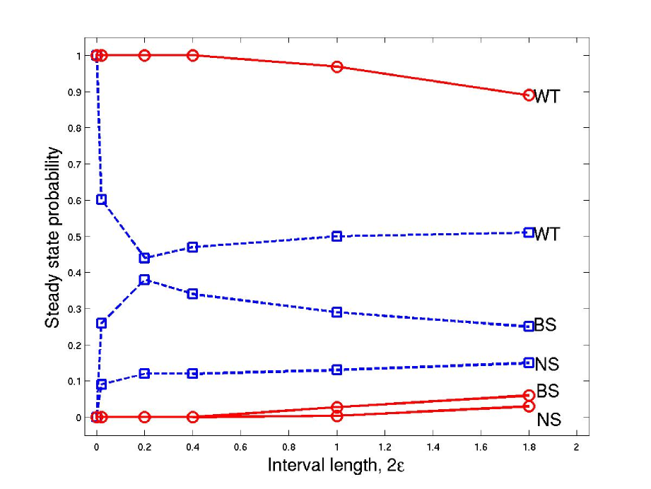
Figure 2: Probability of occurrence of the three most frequent patterns: wild type (WT), broad stripes (BS), and no segmentation (NS), under variable range of timescales. Dashed lines/squares represent asynchronous algorithm results, while solid lines/circles represent Glass-type model results (out of 1000 runs). Results were obtained with $\theta=0.5$.

Note that the case $\varepsilon=0$ reduces to the synchronous model, where every node is updated simultaneously ($\gamma_{i}=1$), at the same time instants: $T_{i}^{k}=k$, for all $i=1,\ldots,N$. This algorithm allows great variability in each process’ duration, exploring the gene expression patterns due to all possible combinations of individual timescales. Implementation of this asynchronous algorithm shows that, if started from the initial wild type state (1), any of the steady states of the model (Table 2) may occur with a certain probability. The probability of occurrence of each pattern depends on the range over which the individual time units $\gamma_{i}$ are allowed to vary (see Fig. 2). For $\varepsilon=0$, the wild type steady state is attained with probability 100% (corresponding to the synchronous Boolean model). As $\varepsilon$ increases to 0.01 (resp. 0.1) this value decreases to 60% (resp. 44%). However, further increase in $\varepsilon$ (hence larger time intervals) unexpectedly leads to an increase in the occurrence of the wild type state, up to 51% for $\varepsilon=0.9$. Other final states observed are the broad-striped pattern ($25\%-38\%$) observed in heat-shock experiments and ptc mutants [17] and the pattern with no segmentation ($12\%-15\%$) observed in en, hh or wg mutants [18], the latter two corresponding to embryonic lethal phenotypes [17]. Each of the other three steady states occurs with frequencies less than $5\%$. (These values were obtained from 10000 numerical experiments.)

A possible extension of this algorithm would be to consider a discrete model with a finite number of logical levels describing ON, OFF as well as other intermediate steps of the system [7]. This would involve decisions about the number of intermediate steps, their values, and development of new transition rules. Instead, in this paper we will focus on a “hybrid” model, that takes into account the continuous nature of the biological processes, while still using Boolean rules to describe ON/OFF transitions (Section 4).

3.1 Random order algorithm

For comparison purposes, we briefly summarize an alternative asynchronous algorithm, which guarantees that every node is updated exactly once during each unit time interval [12]. A random order of updates for the $N$ nodes is generated as a permutation $\phi^{k}$ of $\{1,\ldots N\}$. This permutation is randomly chosen out of a uniform distribution over the set of all $N!$ possible permutations, at the beginning of the time unit $k$. The updating times for each node are now written as

$$T_{i}^{k}=N(k-1)+\phi^{k}(i),\ \ \ k\in{\mathbb{N}},$$

so that $\phi^{k}(j)<\phi^{k}(i)$ implies $T_{j}^{k}<T_{i}^{k}$, and node $j$ is updated before node $i$ at the $k$-th iteration. The results of this algorithm are qualitatively similar to those of the asynchronous algorithm (Table 2).

Table 3: The frequencies of the six steady states observed with the three different methods when starting from the wild type initial condition.

Steady state	Asynchronous	Random order	Glass-type
pattern	algorithm	algorithm	model
wild type	44-51%	56%	89-100%
broad stripes	25-38%	24%	0-6%
no segmentation	12-15%	15%	0-3%
wild type variant	4-5.6%	4.2%	0-1%
ectopic	0.4-1%	0.98%	0%
ectopic variant	0.1-0.5%	0.68%	0%

4 Glass-type networks

The asynchronous algorithm defined by (7), (8) and (9) allows the introduction of distinct timescales for each regulation process in a Boolean model. We next propose an alternative method which provides a bridge between discrete and continuous approaches, resulting in a more realistic model, but without the necessity of specifying any kinetic or binding parameters (which are typically unknown). In this method, the gene and protein levels are represented as continuous variables, and their time evolution is described by differential equations, but the interactions among nodes are still modeled by Boolean functions [13, 14, 15, 23]. Glass [13] introduced a class of piecewise linear differential equations that combine logical rules for the synthesis of gene products with linear (free) decay by describing each node with two variables, one discrete and one continuous. For simplicity of notation, in what follows we will let $\widehat{\mbox{\it X}}_{i}$ denote the continuous variable associated with node $i$, its discrete variable $X_{i}$, and the discrete variable’s Boolean rule by $F_{i}$. The Glass-type model is then

$$\frac{d\,\widehat{\mbox{\it X}}_{i}}{dt}=-\widehat{\mbox{\it X}}_{i}+F_{i}(X_{1},X_{2},\ldots,X_{N}),\ \ \ i=1,\ldots,N.$$ (11)

At each instant $t$, the discrete variable $X_{i}$ is defined as a function of the continuous variable according to a threshold value:

$$X_{i}(t)=\left\{\begin{array}[]{ll}0,&\widehat{\mbox{\it X}}_{i}(t)\leq\theta\\ 1,&\widehat{\mbox{\it X}}_{i}(t)>\theta\ ,\end{array}\right.$$ (14)

where $\theta\in(0,1)$. The discrete variables $X_{i}$ represent the ON and OFF levels of the nodes in the Boolean model. The underlying assumption in this Glass model is that the decay rate and activation threshold of each gene product is identical. Since the initial condition for the piecewise linear system (11) is also (1) (i.e., $X(0)=\widehat{\mbox{\it X}}(0)$) and $F_{i}\in\{0,1\}$, it is easy to see that solutions of (11) evolve in the hypercube $[0,1]^{N}$. Under these conditions, the limiting values “0” and “1” of the continuous variable $\widehat{\mbox{\it X}}_{i}$ represent, respectively, “absence of species $i$” and “maximal concentration of species $i$” – thus we can view the $\widehat{\mbox{\it X}}_{i}$ as dimensionless variables, scaled to attain their maximal values at 1. The continuous dynamics is translated into a Boolean ON/OFF response, according to $\theta$: as soon as $\widehat{\mbox{\it X}}_{i}$ increases above $\theta$, species $i$ is considered to be in the ON state; otherwise it remains in the OFF state (see also [23]). Thus the parameter $\theta$ defines the fraction of “maximal concentration” necessary for a protein or mRNA to effectively perform its biological function. This method allows us to study the continuous evolution of the genetic network simply by specifying $\theta$, the fraction of maximal concentration that is effective as ON level, avoiding the need to specify any kinetic parameters. Below and in Section 6.4, we will see that system (11) exhibits distinct dynamics in the two regions $\theta\leq 1/2$ and $\theta>1/2$. It is easy to see that the steady states of the piecewise linear equations (11) are still those of the Boolean model, since:

$$\frac{d\,\widehat{\mbox{\it X}}_{i}}{dt}=0\ \Leftrightarrow\ \widehat{\mbox{\it X}}_{i}=F_{i}(X_{1},X_{2},\ldots,X_{N}),\ i=1,\ldots,N,$$

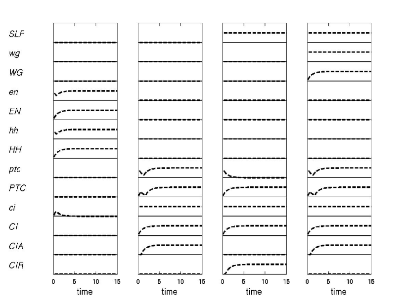
Figure 1: The solution to the system of piecewise linear equations (11) (dashed lines). Each column represents one cell, and each of the 13 rectangles represents the continuous-time variable for proteins or mRNAs (as labeled at left). In each rectangle, the y-axis ranges from 0 to 2 units. The nodes for which the trajectories converge to 1 (middle of the rectangle) are exactly those expressed in the wild type steady state. (The time units are arbitrary.)

independently of $\theta$. Applying this method to the Drosophila segment polarity gene network, we find an exact convergence to the wild type steady state when started from the wild type initial condition (Fig. 1), independently of the ON/OFF threshold value $\theta$. This result supports the Boolean model as a suitable description of the underlying network of gene interactions.

4.1 Introducing distinct timescales

The assumption of equal decay rates and activation thresholds for all nodes is an oversimplification similar to that made in synchronous Boolean models. However, for further robustness analysis, one may introduce different timescales for the different processes, by scaling the time units in each differential equation according to:

$$\frac{d\,\widehat{\mbox{\it X}}_{i}}{dt}=\alpha_{i}(\ -\widehat{\mbox{\it X}}_{i}+F_{i}(X_{1},X_{2},\ldots,X_{N})\ ),$$ (15)

with $\alpha_{i}\geq\varepsilon$ for some fixed $\varepsilon>0$, $i=1,\ldots,N$. Each $X_{i}$ is a discrete variable defined as before (note that steady states of this new system are still those of the Boolean model).

This method represents a continuous equivalent to the asynchronous algorithm described in Section 3. Here, the (inverse) scaling factors $\alpha_{i}^{-1}$ may be viewed as half-lives of mRNA or proteins. These may be directly compared to the individual time units $\gamma_{i}$ as follows. Using Euler’s method to discretize system (15) obtains:

$$\widehat{\mbox{\it X}}_{i}(t+\Delta t)=\widehat{\mbox{\it X}}_{i}(t)+\alpha_{i}\Delta t(-\widehat{\mbox{\it X}}_{i}(t)+F_{i}(X(t))).$$

Now notice that choosing the integrating time interval to be such that $\alpha_{i}\Delta t=1$ recovers the discrete asynchronous algorithm with specific time units

$$\gamma_{i}=\Delta t=\alpha_{i}^{-1}.$$

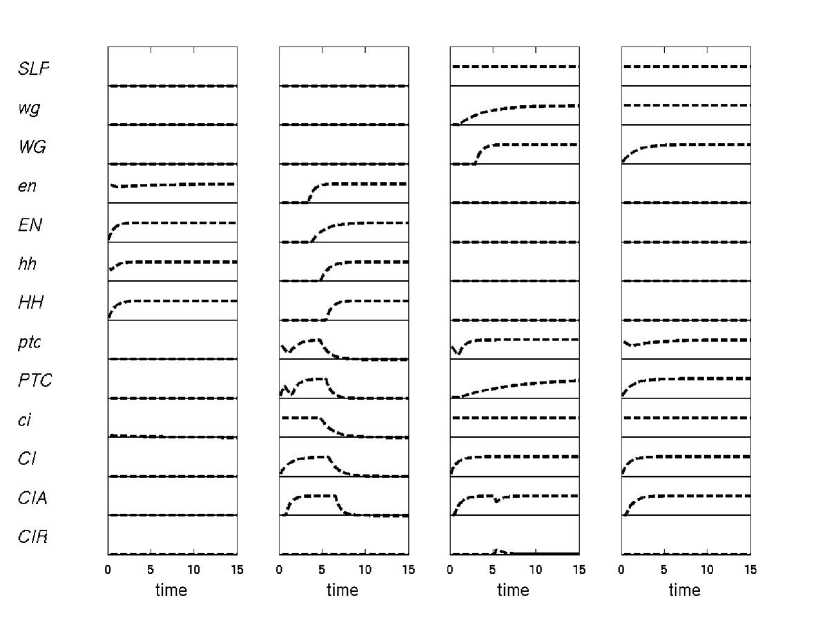
Figure 4: A solution to the system of piecewise linear equations (15) (dashed lines), in an example where the steady state corresponds to the broad stripes pattern. In each rectangle, the y-axis ranges from 0 to 2 units. Notice that wingless is expressed in two adjacent cells, as opposed to the wild type pattern, where wingless is expressed in only one cell (similarly for engrailed and hedgehog).

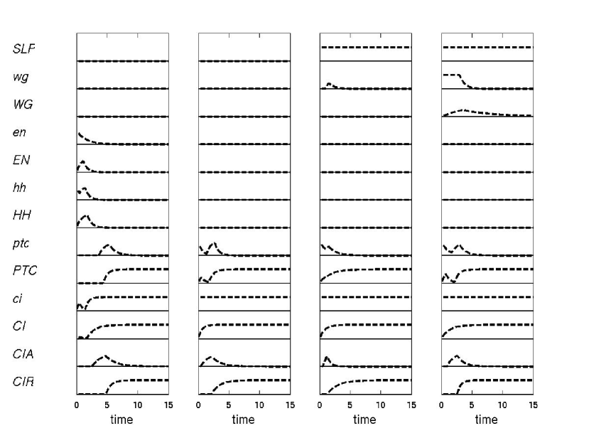
Figure 5: A solution to the system of piecewise linear equations (15) (dashed lines), in an example where the steady state corresponds to the no segmentation pattern. In each rectangle, the y-axis ranges from 0 to 2 units. Notice that wingless, engrailed and hedgehog are not expressed in any cell, thus no segments are visibly detected in the embryo.

For comparison to the discrete algorithm, we choose both the scale factors $\alpha_{i}^{-1}$ and the time units $\gamma_{i}$ randomly from a uniform distribution in intervals of the form $[1-\varepsilon,1+\varepsilon]$, $\varepsilon\in(0,1)$. The numerical experiments are reported in Fig. 2, where the threshold value $\theta$ (14) was set to $1/2$. We again observed that, starting from wild type initial conditions (1), all steady states may occur with a certain frequency (see Table 3). But, in contrast to the asynchronous Boolean model, the wild type pattern occurs with frequencies that decrease monotonically with $\varepsilon$, down to 89% for $\varepsilon=0.9$ (Fig. 2). The next more frequently achieved patterns are the broad stripes (Fig. 4), with probability 6% for $\varepsilon=0.9$, the no segmentation (Fig. 5), with probability 3%, and the wild type variant, with probability 1%.

The three methods we have described (Table 3) produce qualitatively compatible results, in the sense that the wild type pattern is always the most frequently occurring steady state, followed by the broad stripes, no segmentation, and wild type variant patterns.

4.2 Fraction of maximal concentration that defines an ON state

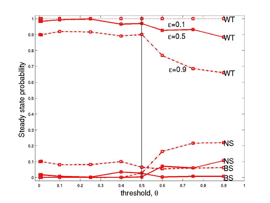
Figure 3: Effect of effective ON concentration, $\theta$, on the probability of occurrence of the three most frequent patterns: wild type (WT), broad stripes (BS), and no segmentation (NS). The results are for the Glass-type model with $\alpha_{i}^{-1}$ randomly chosen in an interval $[1-\varepsilon,1+\varepsilon]$. Solid lines represent the case $\varepsilon=0.5$, dotted lines represent the case $\varepsilon=0.1$ and dash-dotted lines represent the case $\varepsilon=0.9$. (results out of 1000 runs).

The piecewise linear system (15) follows the threshold (14) to decide whether a given node is ON or OFF. While this value $\theta$ did not affect the dynamics of the system in the case $\alpha_{1}=\alpha_{2}=\cdots=\alpha_{N}$, it plays a significant role in the general case. In Figure 3, it is immediate to see that the effect of $\theta$ depends on the length of the interval allowed for the timescales. Indeed, there is a marked difference between narrow ($\varepsilon\leq 0.5$) and wide ($\varepsilon\geq 0.6$) intervals. For narrow intervals, numerical experiments indicate that, starting from initial condition (1), system (15) converges to wild type steady state with probability around 90% or more; whereas, for wider intervals, this probability may decrease down to 68% ($\varepsilon=0.9$, $\theta=0.9$).

On the other hand, the threshold value also divides the dynamics into two regions. For $\theta\leq 0.5$, the probability that initial condition (1) leads to the wild type steady state is above 90%, independently of $\varepsilon$. For $\theta\leq 0.5$ it is less probable to reach the non segmented (around 1%) than the broad striped pattern (around 10%). For higher $\theta\geq 0.6$, the probability of reaching the wild type steady state (from initial condition (1)) decreases very significantly, and in addition, it becomes more problable to reach the non segmented (around 20%) than the broad striped pattern (around 7%).

In our Glass-type model, $\theta$ represents the fraction of maximal concentration above which an mRNA or protein is considered ON, or biologically effective. Our results indicate that quite small fractions of the maximal concentration can (and should) be interpreted as sufficient amounts for an mRNA or protein to be in the ON state. Namely, when the concentration of mRNAs or proteins has increased to a fraction up to half its maximum possible value, it is already present in a sufficient amount to perform its function. This follows from observation of Figure 3: $0<\theta\leq 0.5$ leads to a good (realistic) performance of the model, with 90% convergence to wild type pattern. Our results also indicate that a higher threshold is, on the contrary, not very realistic. For instance, setting $\theta\geq 0.6$ leads to a fairly high incidence on the mutant patterns. But by letting $\theta\geq 0.6$ one is assuming that an mRNA or protein is not present in a sufficient amount to perform its function until it reaches at least sixty per cent of its maximal value. Typically such high thresholds are not observed: indeed, in [11] (supplementary material) where continuous dynamics are also transformed into an ON/OFF response, a threshold of 10% is used, and considered very reasonable. In our experiments, unless otherwise indicated, we have used $\theta=0.5$.

To further generalize system (15), it is natural to allow each variable to respond to its own threshold and consider distinct $\theta_{i}$ values. We will address this problem in Section 6.3, and see that the system’s dynamics is preserved in each $\theta$ region. In fact, our simulations with distinct $\theta_{i}$ recover many of the theoretical results we obtained for a species-independent $\theta$ (Section 6.4).

5 Pre-patterning errors and knockout mutant situations

In [8, 12] we identified some sufficient or necessary initial conditions for obtaining the wild type steady state (minimal pre-patterns). We now analyze how mutant patterns arise from gene “knockout” experiments or delay in establishing the initial pre-pattern.

Gene knockout experiments consist of completely supressing the expression of a given gene in all cells. In our models this is equivalent to setting the corresponding mRNA permanently zero in all equations. Thus a wingless knockout can be analyzed by setting $\mbox{\it wg}_{i}=0$ for all $i=1,2,3,4$, and in every equation of the Boolean rules in Table 1. The steady states of the resulting system can now be computed from:

$$X^{*}=F^{*}(X^{*}),$$ (16)

where the vector $X^{*}$ and functions $F^{*}$ include all but the knockout variables. For example, for the wingless knockout, we drop the functions $F_{\mbox{\tiny\it wg}_{i}}$ and for the other mRNAs and proteins we have

$$\mbox{\it WG}_{i}=F^{*}_{\mbox{\tiny\it WG}_{i}}=0,\ \ i=1,2,3,4$$

$$\mbox{node }=F^{*}_{\mbox{\tiny node}}=F_{\mbox{\tiny node}},\ \mbox{ for nodes }\mbox{\it en},\mbox{\it hh},\mbox{\it ci},\mbox{\it ptc},\mbox{\it EN},\mbox{\it HH},\mbox{\it PTC},\mbox{\it CI},\mbox{\it CIA},\mbox{\it CIR},$$

because wg appears explicitly only in the rules $F_{\mbox{\tiny\it WG}_{i}}$. So, it follows immediately that $\mbox{\it WG}_{i}=0$, and the remaining nodes are then also easy to compute. It is easy to check (see also [8]) that knockouts of wg, en, hh or ptc exhibit only one steady state, while knockouts of ci exhibit three steady states (summarized in Table 4) in both asynchronous and Glass-type models.

Table 4: The steady states corresponding to gene knockouts in the segment polarity network model, calculated according to (16). Here, for the ci knockout, the “wild type” state is interpreted as the wild type pattern in all but the ci, CI, CIA,CIR mRNA/proteins.

Knockouts	Mutant steady states
wg, en, $hh$	no segmentation
ptc	broad stripes
	wild type,
ci	broad stripes ,
	ectopic

From another point of view, one may consider a delay in the establishment of the pre-pattern (that is, the full initial condition (1)). If expression of a given gene is delayed, does the system recover, and how soon? To answer this question, we simulated a delay in expression of gene $X$, by setting the corresponding discrete variable $X(t)=0$ in all cells, for all $t\leq T_{\mbox{\tiny delay}}$. We then varied $T_{\mbox{\tiny delay}}$ between 0 and 7 time units, and measured the frequency of occurrence of each steady state, both for the asynchronous and Glass-type models. (In the latter we set the concentration threshold $\theta$ equal to $1/2$ for all nodes.)

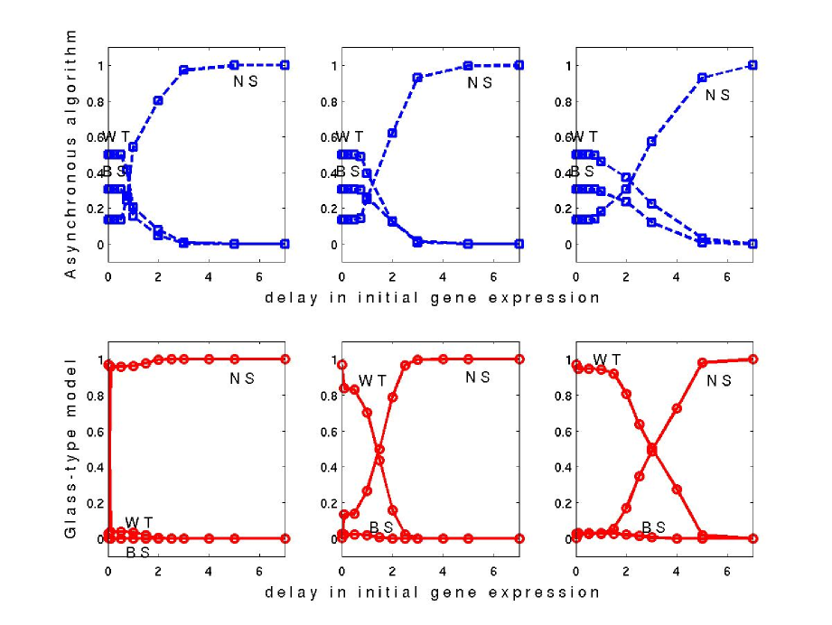
Figure 6: Effect of initially delayed expression in occurrence of steady state patterns. Left: delay in wingless expression. Middle: delay in engrailed expression. Right: delay in hedgehog expression. (results out of 1000 runs).

The results are shown in Figures 6 and 7. We can see that, for short $T_{\mbox{\tiny delay}}$, both models recover their original frequencies of occurrence of each steady state, while for long $T_{\mbox{\tiny delay}}$ both models converge to the corresponding mutant steady state. A curious exception is the case of ci, where long delays in its initial expression do not significantly change the probability that the wild type steady state is achieved (and even slightly increase it in the asynchronous model). This agrees with the conclusion of [8] that cubitus interruptus knockout coupled with an otherwise wild-type initial condition converges to a state close to the wild type steady state. Remarkably, delays in both cubitus interruptus transcription factors (CIA, CIR) have a lesser effect than an imbalance in their expression (see [12]). This leads us to predict that, during the pre-segmentation stage of embryo development, the cubitus interruptus proteins’ expression is the last to be established.

Another noteworthy observation is the fact that small delays in wg expression have much more drastic effects on the system than the same delay in en or hh. This phenomenon reflects the one-way signaling cascade starting with expression of wg, which induces en, which in turn induces hh. We see that a total disruption in the system is caused by a delay of only 3 time units in wg or en expression, which cause the system to fail to reproduce the wild type pattern, and settle into a non-segmented pattern. However, if only hh is delayed, the system is disrupted only after a delay of 5 time units. In other words, recovery of the system back to the “good” developmental process is more probable in the event of a hh expression delay, than a wg or en expression delay.

6 Robustness of the model under timescale separation

In the previous algorithms, the space of all possible timescales for protein/mRNA regulatory processes was explored, with no assumptions on the characteristic duration of translational or post-translational processes. As a consequence, the robustness analysis shows that the model diverges from the wild type pattern very often, with the biologically inviable states occurring with a noticeable frequency. However, it is also well known that post-translational processes such as protein conformational changes or complex formation, usually have shorter durations than transcription, translation or mRNA decay. This fact justifies the introduction of a distinct timescale separation among processes, by choosing to update proteins first and mRNAs later.

6.1 Timescale separation in the random order algorithm

Timescale separation is straightforwardly implemented in the random order algorithm presented in Section 3; at the $k$-th updating step we generate two random permutations, $\phi^{k}_{\mbox{{\tiny\it Prot}}}$ and $\phi^{k}_{\mbox{{\tiny\it mRNA}}}$, within the set of proteins and mRNAs, respectively. Then the $N$ nodes are updated in the order given by

$$\phi^{k}=(\phi^{k}_{\mbox{{\tiny\it Prot}}},\;\phi^{k}_{\mbox{{\tiny\it mRNA}}}).$$

This method again shows that the Boolean model is very robust, in the sense that when started from the wild type initial condition, the wild type pattern occurs with a frequency of $87.5\%$ and only one other steady state is observed, the broad striped pattern, with a frequency of $12.5\%$. Furthermore, these frequencies are exact as we show in [12], where we also completely characterize the model resulting from incorporation of a protein/mRNA timescale separation into the random order algorithm. We show that the wild type state is in fact an attractor for the system, while the pathway to the broad stripes state may exhibit oscillatory cycles. We summarize this and other results in the next theorem, stated without proof, and refer to [12] for more details.

Theorem 1

In the random order algorithm with timescale separation, let $\mbox{\it wg}_{3}^{0}=0$, $\mbox{\it ptc}_{3}^{0}=1$, $\mbox{\it hh}_{2,4}^{0}=0$ and $\mbox{\it ci}_{3}^{0}=1$ (as satisfied by the initial pattern (1)). Then system diverges from the wild type pattern if and only if the permutation $\phi^{1}$ satisfies the following sequence among the proteins CI, CIA, CIR and PTC:

$$\begin{array}[]{cccccc}\mbox{\it CIR}_{3}&\mbox{\it CI}_{3}&&\mbox{\it CIA}_{3}&&\mbox{\it PTC}_{3},\\ &\mbox{\it CI}_{3}&\mbox{\it CIR}_{3}&\mbox{\it CIA}_{3}&&\mbox{\it PTC}_{3},\\ &\mbox{\it CI}_{3}&&\mbox{\it CIA}_{3}&\mbox{\it CIR}_{3}&\mbox{\it PTC}_{3},\end{array}$$ (20)

while the other proteins may appear in any of the remaining slots.  

Thus we can compute the exact probability with which the random order algorithm (with timescale separation) leads to either the wild type or broad stripes pattern: the latter is simply the fraction of sequences of the form (20), and equals $12.5\%$ [12].

6.2 Timescale separation in the Glass-type and asynchronous algorithms

As shown in Section 4, the (discrete) asynchronous algorithm and the (piecewiese continuous) Glass-type system provide equivalent representations of a gene expression network. Indeed, the “specific time units” $\gamma_{i}$ and the inverse “scaling factors” $\alpha_{i}^{-1}$, both represent the rate of dynamical evolution of each individual node. For these two models, we implement time separation among processes by using two non-overlapping intervals for the scaling factors:

$$\gamma_{i}^{-1},\alpha_{i}\in A_{\mbox{{\tiny\it mRNA}}},\ \ \ \mbox{if }\ X_{i}\in\{\mbox{\it wg},\mbox{\it en},\mbox{\it hh},\mbox{\it ptc},\mbox{\it ci}\}$$

$$\gamma_{i}^{-1},\alpha_{i}\in A_{\mbox{{\tiny\it Prot}}},\ \ \ \mbox{if }\ X_{i}\in\{\mbox{\it WG},\mbox{\it EN},\mbox{\it HH},\mbox{\it PTC},\mbox{\it CI},\mbox{\it CIA},\mbox{\it CIR}\},$$

with, for instance, $A_{\mbox{{\tiny\it mRNA}}}=[0.2,0.6]$ and $A_{\mbox{{\tiny\it Prot}}}=[1.4,1.8]$. Under these conditions, choosing the factors $\alpha_{i}$ from a uniform distribution in these intervals, numerical experiments indicate that the two methods respond in mostly similar ways, with only two patterns occurring at steady state when the systems start from (wild type) initial condition (1). The two possible steady states are the wild type and broad stripes patterns.

For the asynchronous algorithm, the probabilities of convergence to each of the steady states clearly depend on the distance between the two intervals: convergence to wild type is $93\%$ in the case where intervals $A_{\mbox{{\tiny\it mRNA}}}$, $A_{\mbox{{\tiny\it Prot}}}$ are consecutive, and up to $100\%$ for the case $2a<b$, $a\in A_{\mbox{{\tiny\it mRNA}}}$, $b\in A_{\mbox{{\tiny\it Prot}}}$.

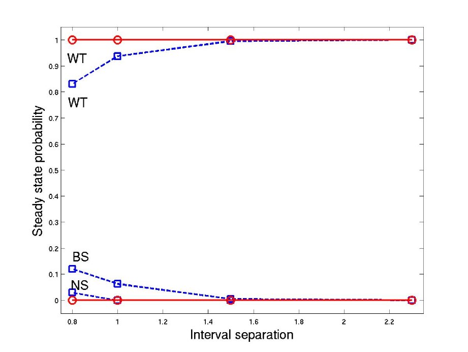
Figure 8: Probability of occurrence of the three most frequent patterns: wild type (WT), broad stripes (BS), and no segmentation (NS), with separation of timescales. Dashed lines/squares represent asynchronous algorithm results, while solid lines/circles represent Glass-type model results. The $x$-axis represents the level of separation, computed by $\min\{b\in A_{\mbox{{\tiny\it Prot}}}\}/\max\{a\in A_{\mbox{{\tiny\it mRNA}}}\}$ (out of 1000 runs). Results were obtained with $\theta=0.5$.

For the Glass-type model, two cases can be distinguished: $\theta\leq 0.5$ and $\theta>0.5$. For $\theta\leq 0.5$, numerical simulations show that the model reaches wild type pattern with probability near 100%, even when there is some overlap between $A_{\mbox{{\tiny\it mRNA}}}$ and $A_{\mbox{{\tiny\it Prot}}}$ (see Fig. 8). In fact, we next theoretically prove that the wild type pattern is indeed the unique possible steady state of the hybrid system (15) and initial condition (1), as indicated by the simulations, when there is a suitable distance between the intervals, and a lower bound on $\theta$ (Theorem 2, Section 6.4). For $\theta>0.5$, we have found no condition that guarantees convergence to the wild type steady state, and indeed numerical simulations show that, even for large interval separation, the system may converge to one of the mutant patterns.

A comparison of Theorems 1 and 2 emphasizes differences and similarities between discrete and continuous models: intuitively, the single discrete event described by Theorem 1 cannot take place in a continuous model. Therefore $\mbox{\it wg}_{3}$ remains “0” (OFF) for all times, ruling out the possibility that the broad stripes pattern is reached. Indeed, Theorem 1 establishes that (in the discrete case, with the random order algorithm) divergence from wild type pattern occurs if and only if $\mbox{\it wg}_{3}^{1}=1$. This fact involves a jump in $\mbox{\it wg}_{3}$ from “0” to “1” at precisely the first iteration. On the other hand, in the Glass-type model, the continuous variable $\widehat{\mbox{\it wg}}_{3}$ cannot instantaneously jump from “0” to “1”. Since the discrete ON/OFF levels are defined by a threshold on $\widehat{\mbox{\it wg}}_{3}$, there will necessarily be a smoothing effect on any transition between “0” and “1”. This is what happens in case (a) of Theorem 2.

The second (sufficient) condition of Theorem 2 guarantees convergence to the wild type steady state for all $0<\theta\leq 0.5$ (while condition (a) is only for $0.382\leq\theta\leq 0.5$), but assumes that $\alpha_{\mbox{\tiny\it PTC}_{3}}>\alpha_{\mbox{\tiny\it CI}_{3}}$. This is an analog to Theorem 1: if $\alpha_{\mbox{\tiny\it PTC}_{3}}>\alpha_{\mbox{\tiny\it CI}_{3}}$, then (starting from $\mbox{\it PTC}_{3}(0)=\mbox{\it CI}_{3}(0)=0$ and assuming $F_{\mbox{\tiny\it PTC}_{3}}=F_{\mbox{\tiny\it CI}_{3}}=1$) $\widehat{\mbox{\it PTC}}_{3}$ increases faster than $\widehat{\mbox{\it CI}}_{3}$, implying that $\mbox{\it PTC}_{3}$ becomes ON faster than $\widehat{\mbox{\it CI}}_{3}$. Such response prevents the events listed in Theorem 1, which would lead to a mutant state. Thus, both discrete and piecewise linear model predict that the sequence of PTC, CI expression in the third cell is one of the fundamental pieces in establishing the correct development of embryo segmentation.

It is also worth pointing out that the three methods provide qualitatively similar results under timescales separation, all predicting that only wild type and broad stripes patterns to occur, the latter with considerably smaller frequency.

Table 5: Probabilities of convergence to a given steady state, under the separation of timescales assumption. These values are theoretically exact for both the random order algorithm and Glass-type model.

Steady state	Random order	Asynchronous	Glass-type
pattern	algorithm	algorithm	model
wild type	87.5%	93.7-100%	100%
broad stripes	12.5%	0-6.3%	0%
other	0%	0%	0%

6.3 Distinct concentration thresholds for ON state

A natural question arising in the analysis of equation (15) concerns the dynamics of the system under more general concentration thresholds. We have seen that $\theta$ (even when equal for all species) plays an important role in establishing basins of attraction to each of the steady states of the model.

We have, in particular, identified three distinct regions of behavior:

$$\begin{array}[]{lc}\mbox{Region 1}:&0<\theta<\frac{3-\sqrt{5}}{2}\\ &\\ \mbox{Region 2}:&\frac{3-\sqrt{5}}{2}\leq\theta\leq\frac{1}{2}\\ &\\ \mbox{Region 3}:&\frac{1}{2}<\theta\leq 1\end{array}$$

When $\theta$ is equal for all nodes, the probability that the system evolves into the wild type pattern is above 90% in regions 1 and 2, but may be as low as 68% in region 3. Furthermore, for region 2, we theoretically prove that that probability is exactly 100% under the timescale separation assumption.

We now associate to each node a specific $\theta_{i}$, so that (14) is modified to:

$$X_{i}(t)=\left\{\begin{array}[]{ll}0,&\widehat{\mbox{\it X}}_{i}(t)\leq\theta_{i}\\ 1,&\widehat{\mbox{\it X}}_{i}(t)>\theta_{i}\ .\end{array}\right.$$ (24)

To test the performance of the system and compare it to previous results, we considered two timescale situations: $\alpha_{i}\in[0.5,1.5]$ for all $i$, or the timescale separation $A_{\mbox{{\tiny\it mRNA}}}=[0.2,0.6]$, $A_{\mbox{{\tiny\it Prot}}}=[1.4,1.8]$. In each case, we randomly assigned values to $\theta_{i}$ from uniform distributions in the intervals $(0,1)$, $(0,0.5)$ and $(0.4,0.5)$. (Note that $0.4$ is close to $(3-\sqrt{5})/2$.) The numerical results with varying $\theta_{i}$ extend and confirm our previous observations for $\theta_{i}=\theta$, $i=1,\ldots,N$.

Table 6 summarizes the results for all combinations of $\theta_{i}$ and $\alpha_{i}$ regions. The most general case, allowing a large degree of freedom in both timescales and concentration thresholds, indicates the vulnerability of the network, with a very high incidence on mutant patterns ($\theta_{i}\in(0,1)$, $\alpha_{i}\in[0.5,1.5]$). Again we see that there is a marked difference in the $\theta_{i}$ regions below or above $0.5$. Comparing the reasonable results obtained for $\theta_{i}\leq 0.5$ with the bad performance for $0.5<\theta_{i}<1$, we conclude that the optimal ON concentratin for proteins or mRNA is below 50% of maximal concentration.

Restricting $\theta_{i}$ even further to one of the conditions given in Theorem 2 (Section 6.4; conditions developed for the case $\theta_{i}=\theta$, $i=1,\ldots,N$) dramatically increases the probability that the system develops in the correct way.

These simulations suggest, moreover, that some of the theoretical results obtained for each of the three regions may extend to the case of distinct $\theta_{i}$. Indeed, note that, under timescale separation, when $\theta_{i}$ are chosen from region 2, convergence to wild type steady state is 100% – compare to part (a) of Theorem 2.

These simulations further confirm the role of $\alpha_{\mbox{\tiny\it PTC}_{3}}$ and $\alpha_{\mbox{\tiny\it CI}_{3}}$ in the segmentation network. Requiring $\alpha_{\mbox{\tiny\it PTC}_{3}}>\alpha_{\mbox{\tiny\it CI}_{3}}$ decreases the probability of formation of the broad stripes pattern (any timescales), but doesn’t influence the probability of a non segmented embryo. The latter mutant is prevented only by a complete separation of timescales of the regulatory processes.

Table 6: Probabilities of convergence to a given steady state, with distinct concentration thresholds $\theta_{i}$ and distinct timescales $\alpha_{i}$, in the Glass-type model. (Probabilities computed out of 1000 simulations for each case.)

Steady state	$(0,1)$	$(0.5,1)$	$(0,0.5]$	$(0,0.5]$	$[0.4,0.5]$	$0.5$	$\theta_{i}$
pattern				$\alpha_{\mbox{\tiny\it PTC}_{3}}>\alpha_{\mbox{\tiny\it CI}_{3}}$			$\alpha_{i}$
wild type	45.6%	57.1%	84.1%	90%	92.6%	94.2%	$A_{\mbox{{\tiny\it mRNA}}}=$
broad stripes	27.8%	15.1%	12%	6.2%	7.3%	4.5%	$A_{\mbox{{\tiny\it Prot}}}=$
no segmentation	24.4%	25.8%	0.9%	0.9%	0.05%	1.3%	$[0.5,1.5]$
wild type, variant	2.1%	1.9%	2.9%	2.9%	0%	0%
wild type	74.1%	52.7%	96.6%	97.1%	100%	100%	$A_{\mbox{{\tiny\it mRNA}}}=$
broad stripes	10.8%	3.3%	3.3%	2.8%	0%	0%	$[0.2,0.6]$
no segmentation	14.1%	43.9%	0%	0%	0%	0%	$A_{\mbox{{\tiny\it Prot}}}=$
wild type, variant	1.0%	0%	0.1%	0.1%	0%	0%	$[1.4,1.8]$

6.4 Glass-type model provides exact convergence to wild type pattern

In this section we will require that the intervals $A_{\mbox{{\tiny\it mRNA}}}$ and $A_{\mbox{{\tiny\it Prot}}}$ do not overlap, by satisfying the following assumption:

$$\mbox{For all }\ \ a\in A_{\mbox{{\tiny\it mRNA}}}\ \ \mbox{and}\ \ b\in A_{\mbox{{\tiny\it Prot}}}:\ \ \ 0<2a<b.$$ (25)

A second assumption is that the effective maximal concentration is equal for all nodes and satisfies $\theta\leq 1/2$, which is equivalent to:

$$\ln\frac{1}{1-\theta}\leq\ln\frac{1}{\theta}$$ (26)

Theorem 2

Consider system (15) with initial condition (1). Assume that the scaling factors $\alpha_{i}$ satisfy (25). Assume also that one of the following conditions holds:

• $\theta\leq 1/2$ and $(1-\theta)^{2}\leq\theta$ or equivalently $0.382\approx(3-\sqrt{5})/2\leq\theta\leq 1/2$;

• $\theta\leq 1/2$ and $\alpha_{\mbox{\tiny\it PTC}_{3}}>\alpha_{\mbox{\tiny\it CI}_{3}}$;

then $\mbox{\it wg}_{3}(t)=0$ for all $t$.

This shows that the steady state representing the broad stripes pattern cannot ever be reached in system (15) from the initial condition (1), when $\theta\leq 1/2$ and either of the extra conditions holds.

Theorem 3

Consider system (15) with initial condition (1). Assume that the scaling factors $\alpha_{i}$ satisfy (25), and that $\theta\leq 1/2$. Then $\mbox{\it wg}_{4}(t)=1$ and $\mbox{\it PTC}_{1}(t)=0$ for all $t$.

This shows that the steady states represented by the no segmentation, wild type variant or the two ectopic patterns also cannot ever be reached in system (15) from the initial condition (1). From Theorems 2 and 3 we conclude that, under the timescale separation assumption, the Glass-type model (15) can only converge to the wild type pattern, when starting from the initial condition (1), and for appropriate $\theta$ values (Table 5).

We first summarize some useful observations. Let $X$ denote any of the nodes in the network, and $\alpha$ its time rate. Since equations (15) are either of the form $d\widehat{\mbox{\it X}}/dt=\alpha(-\widehat{\mbox{\it X}}+1)$ or $d\widehat{\mbox{\it X}}/dt=-\alpha\widehat{\mbox{\it X}}$, their solutions are continous functions, piecewise combinations of:

$$\widehat{\mbox{\it X}}^{1}(t) = 1-(1-\widehat{\mbox{\it X}}^{1}(t_{0}))\,e^{-\alpha(t-t_{0})}$$ (27)

$$\widehat{\mbox{\it X}}^{0}(t) = \widehat{\mbox{\it X}}^{0}(t_{0})\,e^{-\alpha(t-t_{0})}$$ (28)

$\widehat{\mbox{\it X}}^{1}(t)$ (resp. $\widehat{\mbox{\it X}}^{0}(t)$) is monotonically increasing (resp. decreasing). In addition, note that discrete variables $X$ can only switch between 0 and 1 at those instants when $\widehat{\mbox{\it X}}(t_{\mbox{\tiny switch}})=\theta$, that is:

$$t_{\mbox{\tiny switch}}^{1} = t_{0}+\frac{1}{\alpha}\,\ln\,\frac{{(1-\widehat{\mbox{\it X}}(t_{0}))}}{1-\theta}$$ (29)

$$t_{\mbox{\tiny switch}}^{0} = t_{0}+\frac{1}{\alpha}\,\ln\,\frac{{\widehat{\mbox{\it X}}(t_{0})}}{\theta}$$ (30)

From the initial conditions, together with the constant values of $\mbox{\it SLP}_{i}$ ($i=1,2,3,4$), we can immediately conclude:

$$\widehat{\mbox{\it wg}}_{1,2}(t)=\mbox{\it WG}_{1,2}(t)=0,$$ (31)

$$\widehat{\mbox{\it en}}_{3,4}(t)=\widehat{\mbox{\it EN}}_{3,4}(t)=0,$$

$$\widehat{\mbox{\it hh}}_{3,4}(t)=\widehat{\mbox{\it HH}}_{3,4}(t)=0,$$ (32)

for all $t\geq 0$. Then, because $\mbox{\it ci}_{3,4}(0)=1$ and $F_{\mbox{\tiny\it ci}_{3,4}}=\mbox{not }\mbox{\it EN}_{3,4}$,

$$\widehat{\mbox{\it ci}}_{3,4}(t)=1\ \mbox{ and }\ \widehat{\mbox{\it CI}}_{3,4}(t)=1-e^{-\alpha_{\mbox{\tiny\it CI}_{3,4}}\,t}.$$ (33)

Lemma 6.1

Let $0\leq t_{0}<t_{3}\leq t_{1}$ and $0\leq t_{2}<t_{3}$. Define $\delta=\ln\frac{1}{1-\theta}/\max_{1,\ldots,N}{\alpha_{i}}$. Assume $\mbox{\it CIA}_{3}(t)=0$ for $t\in(t_{2},t_{3})$, and $\mbox{\it wg}_{3}(t)=0$ for $t\in[0,t_{3})$. Then

• $\mbox{\it wg}_{3}(t)=0$ for $t\in[0,t_{3}+\delta)$;

• $\mbox{\it WG}_{3}(t)=0$ for $t\in[0,t_{3}+\delta)$;

• $\mbox{\it en}_{2}(t)=\mbox{\it EN}_{2}(t)=0$ for $t\in[0,t_{3}+\delta)$;

• $\mbox{\it hh}_{2}(t)=\mbox{\it HH}_{2}(t)=0$ for $t\in[0,t_{3}+\delta)$.

Assume further that $\mbox{\it PTC}_{3}(t)=1$ for $t\in(t_{0},t_{1})$. Then

• $\mbox{\it PTC}_{3}(t)=1$ for all $t\in(t_{0},t_{3}+\delta)$.

• $\mbox{\it CIA}_{3}(t)=0$ for all $t\in(t_{2},t_{3}+\delta)$.

Proof: Part (a) follows directly from the fact that $F_{\mbox{\tiny\it wg}_{3}}(t)=0$ on $[0,t_{3})$, and from (29).

To prove parts (b), (c), and (d), first note that initial conditions together with $\mbox{\it wg}_{3}(t)=0$ for $t\in[0,t_{3})$ imply

$$\widehat{\mbox{\it WG}}_{3}(t)=0,\ \widehat{\mbox{\it en}}_{2}(t)=\widehat{\mbox{\it EN}}_{2}(t)=0,$$

$$\widehat{\mbox{\it hh}}_{2}(t)=\widehat{\mbox{\it HH}}_{2}(t)=0,$$

for $t\in[0,t_{3}]$. Then, from equations (27) to (30) we conclude that the corresponding discrete variables cannot switch from 0 to 1 during an interval of the form $[0,t_{3}+\frac{1}{\alpha_{j}}\ln\frac{1}{1-\theta})$. Taking the largest common interval yields the desired results.

To prove parts (e) and (f), assume also that $\mbox{\it PTC}_{3}(t)=1$ for $t\in(t_{0},t_{1})$. From (32) and part (d), it follows that function $F_{\mbox{\tiny\it PTC}_{3}}$ does not switch in the interval $(t_{0},t_{3}+\delta)$ and in fact $\mbox{\it PTC}_{3}(t)=1$ for all $t$ in this interval. This, together with (32) and part (d) yield $F_{\mbox{\tiny\it CIA}_{3}}(t)=0$ for $(t_{0},t_{3}+\delta)$, so that $\widehat{\mbox{\it CIA}}_{3}$ cannot increase in this interval and the discrete level satisfies $\mbox{\it CIA}_{3}(t)=0$ for all $t\in(t_{2},t_{3}+\delta)$, as we wanted to show.  

Corollary 6.2

Let $0\leq t_{0}<t_{3}\leq t_{1}$ and $0\leq t_{2}<t_{3}$. If $\mbox{\it PTC}_{3}(t)=1$ for $t\in(t_{0},t_{1})$, $\mbox{\it CIA}_{3}(t)=0$ for $t\in(t_{2},t_{3})$, and $\mbox{\it wg}_{3}(t)=0$ for $t\in[0,t_{3})$, then $\mbox{\it wg}_{3}(t)=0$ for all $t$.

Proof: Applying Lemma 6.1 we conclude that, given any $k\geq 0$:

$$\mbox{\it CIA}_{3}(t)=0,\ \mbox{ for }\ t\in(t_{2},t_{3}+k\delta)$$

$$\mbox{\it wg}_{3}(t)=0,\ \mbox{ for }\ t\in[0,t_{3}+k\delta)$$

$$\mbox{\it PTC}_{3}(t)=1\ \mbox{ for }\ t\in(t_{0},t_{3}+k\delta)$$

imply

$$\mbox{\it CIA}_{3}(t)=0,\ \mbox{ for }\ t\in(t_{2},t_{3}+(k+1)\delta)$$

$$\mbox{\it wg}_{3}(t)=0,\ \mbox{ for }\ t\in[0,t_{3}+(k+1)\delta)$$

$$\mbox{\it PTC}_{3}(t)=1\ \mbox{ for }\ t\in(t_{0},t_{3}+(k+1)\delta).$$

Since $\delta$ is finite, we conclude by induction on $k$ that $\mbox{\it wg}_{3}(t)=0$ for all $t$.  

Proof of Theorem 2: The rule for $\mbox{\it CIA}_{3}$ may be simplified to (by (32))

$$F_{\mbox{\tiny\it CIA}_{3}}=\mbox{\it CI}_{3}\mbox{ and }[\mbox{not}\mbox{\it PTC}_{3}\mbox{ or }\mbox{\it hh}_{2}\mbox{ or }\mbox{\it HH}_{2}].$$

From equation (33), we have that

$$\mbox{\it CI}_{3}(t)=1,\ \mbox{ for all }t>\frac{1}{\alpha_{\mbox{\tiny\it CI}_{3}}}\ln\frac{1}{1-\theta}.$$ (34)

On the other hand, since $\mbox{\it ptc}_{3}(0)=1$, by continuity of solutions $\mbox{\it ptc}_{3}(t)=1$ for all $t<\frac{1}{\alpha_{\mbox{\tiny\it ptc}_{3}}}\ln\frac{1}{\theta}$. This implies that the Patched protein satisfies

$$\widehat{\mbox{\it PTC}}_{3}(t)=1-e^{-\alpha_{\mbox{\tiny\it PTC}_{3}}\,t},\ \ 0\leq t\leq\frac{1}{\alpha_{\mbox{\tiny\it ptc}_{3}}}\ln\frac{1}{\theta}$$

and therefore

$$\mbox{\it PTC}_{3}(t)=\left\{\begin{array}[]{ll}0,&0\leq t\leq\frac{1}{\alpha_{\mbox{\tiny\it PTC}_{3}}}\ln\frac{1}{1-\theta}\\ 1,&\frac{1}{\alpha_{\mbox{\tiny\it PTC}_{3}}}\ln\frac{1}{1-\theta}<t<\frac{1}{\alpha_{\mbox{\tiny\it ptc}_{3}}}\ln\frac{1}{\theta}.\end{array}\right.$$ (37)

By assumption, $\alpha_{\mbox{\tiny\it PTC}_{3}}>\alpha_{\mbox{\tiny\it ptc}_{3}}$ and also $\ln\frac{1}{1-\theta}\leq\ln\frac{1}{\theta}$, defining a nonempty interval where $\mbox{\it PTC}_{3}$ is expressed. Now let $t_{c}=\frac{1}{\alpha_{\mbox{\tiny\it CI}_{3}}}\ln\frac{1}{1-\theta}$ and $t_{p}=\frac{1}{\alpha_{\mbox{\tiny\it PTC}_{3}}}\ln\frac{1}{1-\theta}$. $\widehat{\mbox{\it CIA}}_{3}(t)$ starts at zero and must remain so while $\mbox{\it CI}_{3}=0$, so that

$$\mbox{\it CIA}_{3}(t)=0\ \mbox{ for }0<t<t_{c}.$$

In the case $t_{c}>t_{p}$, letting $t_{0}=t_{p}$, $t_{1}=\frac{1}{\alpha_{\mbox{\tiny\it ptc}_{3}}}\ln\frac{1}{\theta}$, $t_{2}=0$, and $t_{3}=t_{c}$ in Corollary 6.2, obtains $\mbox{\it wg}_{3}(t)=0$ for all $t$. This proves item (b) of the theorem, and part of (a).

To finish the proof of item (a), we assume that $(1-\theta)^{2}<\theta$ and must now consider the case $t_{c}\leq t_{p}$. Then

$$\widehat{\mbox{\it CIA}}_{3}(t)=\left\{\begin{array}[]{ll}0,&0\leq t\leq t_{c}\\ 1-e^{-\alpha_{\mbox{\tiny\it CIA}_{3}}\,(t-t_{c})},&t_{c}<t\leq t_{p}\\ \widehat{\mbox{\it CIA}}_{3}(t_{p})\,e^{-\alpha_{\mbox{\tiny\it CIA}_{3}}\,(t-t_{p})},&t_{p}<t\leq\frac{1}{\alpha_{\mbox{\tiny\it ptc}_{3}}}\ln\frac{1}{\theta},\end{array}\right.$$

Following equation (29) with $t_{0}=t_{c}$ and $\widehat{\mbox{\it CIA}}_{3}(t_{0})=0$, $\mbox{\it CIA}_{3}$ might become expressed at time $t_{c}<t_{a}<t_{p}$:

$$t_{a}=t_{c}+\frac{1}{\alpha_{\mbox{\tiny\it CIA}_{3}}}\ln\frac{1}{1-\theta},$$

but it would then become zero again at (equation (30) with $t_{0}=t_{p}$)

$$t_{b}=t_{p}+\frac{1}{\alpha_{\mbox{\tiny\it CIA}_{3}}}\ln\,\frac{{\widehat{\mbox{\it CIA}}_{3}(t_{p})}}{\theta}.$$

Finally, we show that, even if $\mbox{\it CIA}_{3}(t)=1$ for $t\in(t_{a},t_{b})$, $\mbox{\it wg}_{3}$ cannot become expressed in this interval. In this interval, $\widehat{\mbox{\it wg}}_{3}$ evolves according to $\widehat{\mbox{\it wg}}_{3}(t)=1-e^{-\alpha_{\mbox{\tiny\it wg}_{3}}\,(t-t_{a})},$ and $\mbox{\it wg}_{3}$ can switch to 1 at time

$$t_{w}=t_{a}+\frac{1}{\alpha_{\mbox{\tiny\it wg}_{3}}}\ln\frac{1}{1-\theta}.$$

We will show that $t_{w}>t_{b}$, so $\mbox{\it wg}_{3}(t)=0$ in the interval $[0,t_{b})$. Writing

$$\ln\,\frac{{\widehat{\mbox{\it CIA}}_{3}(t_{p})}}{\theta} = \ln\,\frac{{\widehat{\mbox{\it CIA}}_{3}(t_{p})}}{1-\theta}\frac{1-\theta}{\theta}$$

$$= \ln\,\frac{{\widehat{\mbox{\it CIA}}_{3}(t_{p})}}{1-\theta}+\ln\,\frac{1-\theta}{\theta}$$

$$\leq \ln\frac{1}{1-\theta}+\ln\frac{1}{1-\theta}$$

where we have used $\widehat{\mbox{\it CIA}}_{3}(t_{p})\leq 1$ and the assumption on $\theta$: $\frac{1-\theta}{\theta}\leq\frac{1}{1-\theta}$. Therefore

$$t_{b} \leq t_{p}+\frac{2}{\alpha_{\mbox{\tiny\it CIA}_{3}}}\ln\frac{1}{1-\theta}$$

$$< \frac{1}{\alpha_{\mbox{\tiny\it wg}_{3}}}\ln\frac{1}{1-\theta}+\frac{1}{\alpha_{\mbox{\tiny\it CIA}_{3}}}\ln\frac{1}{1-\theta}<t_{w}$$

where we have used the timescale separation assumption (25). Letting $t_{0}=t_{p}$, $t_{2}=0$, and $t_{1}=t_{3}=\min\{t_{b},\alpha_{\mbox{\tiny\it ptc}_{3}}^{-1}\ln\frac{1}{\theta}\}$ in the Corollary, obtains $\mbox{\it wg}_{3}(t)=0$ for all $t$.  

We will next show that if $\mbox{\it wg}_{4}(t)=1$ in a given interval $[0,T)$, then in fact $\mbox{\it wg}_{4}(t)$ remains expressed for a longer time, up to $T+\delta$, with $\delta>0$. This is mainly due to assumption (25), which says that mRNAs take longer than proteins to update their discrete values, because they have longer half-lives: $\alpha_{\mbox{{\tiny\it mRNA}}}^{-1}>\alpha_{\mbox{{\tiny\it Prot}}}^{-1}$. This allows the initial signal “$\mbox{\it wg}_{4}=1$” to travel down the network, sequencially affecting the wingless protein, engrailed, hedgehog and CIA, and feed back into wingless allowing $\mbox{\it wg}_{4}$ to remain expressed for a further time interval.

Lemma 6.3

Let $T\geq\frac{1}{\alpha_{\mbox{\tiny\it wg}_{4}}}\ln\frac{1}{\theta}$ and define

$$\delta=\frac{1}{\alpha_{\mbox{\tiny\it WG}_{4}}}\,\ln\,\frac{{(1-e^{-\frac{\alpha_{\mbox{\tiny\it WG}_{4}}}{\alpha_{\mbox{\tiny\it wg}_{4}}}\ln\frac{1}{\theta}})}}{\theta}.$$ (39)

If $\mbox{\it wg}_{4}(t)=1$ for $0\leq t<T$, then

• $\mbox{\it WG}_{4}(t)=1$ for $t\in(\frac{1}{\alpha_{\mbox{\tiny\it WG}_{4}}}\ln\frac{1}{1-\theta},T+\delta)$;

• $\mbox{\it en}_{1}(t)=1$ for $t\in[0,T+\delta)$;

• $\widehat{\mbox{\it EN}}_{1}(t)=1-e^{-\alpha_{\mbox{\tiny\it EN}_{1}}t}$ for $t\in[0,T+\delta)$, and $\mbox{\it EN}_{1}(t)=1$ for $(\frac{1}{\alpha_{\mbox{\tiny\it EN}_{1}}}\ln\frac{1}{1-\theta},T+\delta)$;

• $\mbox{\it ci}_{1}(t)=0$, $\mbox{\it CI}_{1}(t)=0$, $\mbox{\it CIA}_{1}(t)=0$, and $\mbox{\it CIR}_{1}(t)=0$ for $t\in[0,T+\delta)$;

• $\mbox{\it hh}_{1}(t)=1$, for $t\in[0,T+\delta)$;

• $\mbox{\it CIA}_{4}(t)=1$, for $t\in(\frac{1}{\alpha_{\mbox{\tiny\it CI}_{4}}}\ln\frac{1}{1-\theta}+\frac{1}{\alpha_{\mbox{\tiny\it CIA}_{4}}}\ln\frac{1}{1-\theta},T+\delta)$, and $\mbox{\it CIR}_{4}(t)=0$, for $t\in[0,T+\delta)$;

• $\mbox{\it wg}_{4}(t)=1$ for $t\in[0,T+\delta)$.

Proof: Let $T\geq\frac{1}{\alpha_{\mbox{\tiny\it wg}_{4}}}\ln\frac{1}{\theta}$, and assume that $\mbox{\it wg}_{4}(t)=1$ for $0\leq t<T$. To prove part (a), note that $\widehat{\mbox{\it WG}}_{4}(t)$ is of the form (27) (with $t_{0}=0$, and $\widehat{\mbox{\it WG}}_{4}(0)=0$) and the corresponding discrete variable is $\mbox{\it WG}_{4}(t)=1$, for $t\in(\frac{1}{\alpha_{\mbox{\tiny\it WG}_{4}}}\ln\frac{1}{1-\theta},T)$. Moreover, suppose that $\mbox{\it wg}_{4}(t)=0$ for $t>T$, then

$$\widehat{\mbox{\it WG}}_{4}(t)=(1-e^{-\alpha_{\mbox{\tiny\it WG}_{4}}T})e^{-\alpha_{\mbox{\tiny\it WG}_{4}}(t-T)},\ \ \ t>T.$$

But $\mbox{\it WG}_{4}$ remains 1 until the switching threshold is attained, that is up to time

$$T+\frac{1}{\alpha_{\mbox{\tiny\it WG}_{4}}}\ln\,\frac{{(1-e^{-\alpha_{\mbox{\tiny\it WG}_{4}}T})}}{\theta}$$

$$\geq T+\frac{1}{\alpha_{\mbox{\tiny\it WG}_{4}}}\ln\,\frac{{(1-e^{-\alpha_{\mbox{\tiny\it WG}_{4}}\frac{1}{\alpha_{\mbox{\tiny\it wg}_{4}}}\ln\frac{1}{\theta}})}}{\theta}$$

$$\equiv T+\delta.$$

Thus we conclude that $\mbox{\it WG}_{4}(t)=1$ in the desired interval.

To prove part (b), observe that $F_{\mbox{\tiny\it en}_{1}}(t)=\mbox{\it WG}_{4}(t)$ for all $t$, from (31), and recall that $\mbox{\it en}_{1}(0)=1$. From part (a), $F_{\mbox{\tiny\it en}_{1}}(t)=1$ for $t\in(\frac{1}{\alpha_{\mbox{\tiny\it WG}_{4}}}\ln\frac{1}{1-\theta},T+\delta)$. On the other hand, $\mbox{\it en}_{1}$ can only switch from 1 to 0 at $t=\alpha_{\mbox{\tiny\it en}_{1}}^{-1}\ln\frac{1}{\theta}$ which is larger than $\alpha_{\mbox{\tiny\it WG}_{4}}^{-1}\ln\frac{1}{1-\theta}$. So, in fact, $\mbox{\it en}_{1}(t)=1$ for all $0\leq t<T+\delta$.

Part (c) follows immediately by integration of the $\widehat{\mbox{\it EN}}_{1}$ equation.

To prove part (d), first recall $F_{\mbox{\tiny\it ci}_{1}}=$ not $\mbox{\it EN}_{1}$ and the initial conditions $\mbox{\it ci}_{1}(0)=0=\mbox{\it CI}_{1}(0)=\mbox{\it CIA}_{1}(0)=\mbox{\it CIR}_{1}(0)$. Therefore $\widehat{\mbox{\it ci}}_{1}(t)$ increases up to $t=\frac{1}{\alpha_{\mbox{\tiny\it EN}_{1}}}\ln\frac{1}{1-\theta}$ and then decreases in $\alpha_{\mbox{\tiny\it EN}_{1}}^{-1}\ln\frac{1}{1-\theta}<t<T+\delta$. Now note that the discrete variable $\mbox{\it ci}_{1}(t)$ remains 0 in the whole interval $[0,T+\delta)$. This is because $\widehat{\mbox{\it ci}}_{1}$ never reaches the $\theta$ threshold: this would be attained at some $t\geq\alpha_{\mbox{\tiny\it ci}_{1}}^{-1}\ln\frac{1}{1-\theta}$ but, since $\alpha_{\mbox{\tiny\it ci}_{1}}^{-1}\ln\frac{1}{1-\theta}>\alpha_{\mbox{\tiny\it EN}_{1}}^{-1}\ln\frac{1}{1-\theta}$, the function $\widehat{\mbox{\it ci}}_{1}$ starts decreasing before it could reach the value $\theta$. Finally, from the rules of the Cubitus proteins it is immediate to see that $\mbox{\it CI}_{1}(t)=\mbox{\it CIA}_{1}(t)=\mbox{\it CIR}_{1}(t)=0$ for $t\in[0,T+\delta)$.

To prove part (e), recall that $F_{\mbox{\tiny\it hh}_{1}}=\mbox{\it EN}_{1}$ and not $\mbox{\it CIR}_{1}$. From part (a), it follows that $F_{\mbox{\tiny\it hh}_{1}}(t)=0$ in the interval $[0,\alpha_{\mbox{\tiny\it EN}_{1}}^{-1}\ln\frac{1}{1-\theta})$ and $F_{\mbox{\tiny\it hh}_{1}}(t)=1$ in the interval $(\alpha_{\mbox{\tiny\it EN}_{1}}^{-1}\ln\frac{1}{1-\theta},T+\delta)$. Since $\mbox{\it hh}_{1}(0)=1$, $\widehat{\mbox{\it hh}}_{1}(t)$ decreases in the interval $[0,\alpha_{\mbox{\tiny\it EN}_{1}}^{-1}\ln\frac{1}{1-\theta})$ but increases in $(\alpha_{\mbox{\tiny\it EN}_{1}}^{-1}\ln\frac{1}{1-\theta},T+\delta)$. The discrete value is $\mbox{\it hh}_{1}(t)=1$ in the whole interval, since $\widehat{\mbox{\it hh}}_{1}(t)$ remains above the $\theta$ threshold. (The justification is similar to the case of $\mbox{\it ci}_{1}(t)$ in part (d).)

To prove part (f), note that part (e) and then the use of (33), allows us to simplify $F_{\mbox{\tiny\it CIA}_{4}}$:

$$F_{\mbox{\tiny\it CIA}_{4}}(t)=\mbox{\it CI}_{4}(t)\ \mbox{ and }\ \mbox{\it hh}_{1}(t)=1,\ \ \ t\in(\frac{1}{\alpha_{\mbox{\tiny\it CI}_{4}}}\ln\frac{1}{1-\theta},T+\delta).$$

Thus

$$\widehat{\mbox{\it CIA}}_{4}(t)=\left\{\begin{array}[]{ll}0,&0\leq t\leq\frac{1}{\alpha_{\mbox{\tiny\it CI}_{4}}}\ln\frac{1}{1-\theta}\\ 1-e^{-\alpha_{\mbox{\tiny\it CIA}_{4}}\left(t-\frac{1}{\alpha_{\mbox{\tiny\it CI}_{4}}}\ln\frac{1}{1-\theta}\right)},&\frac{1}{\alpha_{\mbox{\tiny\it CI}_{4}}}\ln\frac{1}{1-\theta}<t\leq T+\delta,\end{array}\right.$$

and $\mbox{\it CIA}_{4}(t)=1$ for $t\in[\frac{1}{\alpha_{\mbox{\tiny\it CI}_{4}}}\ln\frac{1}{1-\theta}+\frac{1}{\alpha_{\mbox{\tiny\it CIA}_{4}}}\ln\frac{1}{1-\theta},T+\delta)$. Observe that this interval is indeed nonempty, by assumption (25). Finally, $F_{\mbox{\tiny\it CIR}_{4}}(t)=\mbox{\it CI}_{4}(t)\mbox{ and not}\mbox{\it hh}_{1}(t)=0$, and hence $\mbox{\it CIR}_{4}(t)=0$ for $t\in[0,T+\delta)$.

To prove part (g), we note that (from part (f))

$$F_{\mbox{\tiny\it wg}_{4}}(t)=1,\ \ \ t\in(\frac{1}{\alpha_{\mbox{\tiny\it CI}_{4}}}\ln\frac{1}{1-\theta}+\frac{1}{\alpha_{\mbox{\tiny\it CIA}_{4}}}\ln\frac{1}{1-\theta},T+\delta),$$

implying that $\widehat{\mbox{\it wg}}_{4}(t)$ increases in this interval. On the other hand, we know that $\widehat{\mbox{\it wg}}_{4}(t)\geq\theta$ and $\mbox{\it wg}_{4}(t)=1$ up to at least $t=\frac{1}{\alpha_{\mbox{\tiny\it wg}_{4}}}\ln\frac{1}{\theta}>\frac{1}{\alpha_{\mbox{\tiny\it CI}_{4}}}\ln\frac{1}{1-\theta}+\frac{1}{\alpha_{\mbox{\tiny\it CIA}_{4}}}\ln\frac{1}{1-\theta}$. This shows that in fact $\mbox{\it wg}_{4}(t)=1$ for all $t\in[0,T+\delta)$.  

Proof of Theorem 3: Since $\mbox{\it wg}_{4}(0)=1$, from equations (29), (30), we know that the earliest possible switching time from 1 to 0 is $\alpha_{\mbox{\tiny\it wg}_{4}}^{-1}\ln\frac{1}{\theta}$. Applying Lemma 6.3 with $T=\alpha_{\mbox{\tiny\it wg}_{4}}^{-1}\ln\frac{1}{\theta}$ establishes that $\mbox{\it wg}_{4}(t)=1$ for $t\in[0,T+\delta)$, with $\delta$ given by (39). Next, applying Lemma 6.3 with $T=\alpha_{\mbox{\tiny\it wg}_{4}}^{-1}\ln\frac{1}{\theta}+k\delta$, $k\in{\mathbb{N}}$, shows that $\mbox{\it wg}_{4}(t)=1$ for $t\in[0,T+(k+1)\delta)$. Since $\delta$ is finite, we can conclude by induction that $\mbox{\it wg}_{4}(t)=1$ for all $t\geq 0$.

To prove that $\mbox{\it PTC}_{1}(t)\equiv 0$, note that $\mbox{\it CIA}_{1}(t)\equiv 0$ (Lemma 6.3, with $T=+\infty$) implies $\mbox{\it ptc}_{1}(t)\equiv 0$. Since $\mbox{\it PTC}_{1}(0)=0$ and $\mbox{\it PTC}_{1}$ cannot become expressed unless $\mbox{\it ptc}_{1}$ is first expressed, the desired result follows.  

7 Conclusions

We discussed two alternative methods for modeling gene expression networks: purely discrete Boolean methods and piecewise linear differential systems, which combine continuous degradation with discrete synthesis. For both methods we introduced new techniques for a deeper analysis of the networks with respect to perturbations in the timescales of the system. For the piecewise linear system we also studied the effect of the ON concentration thresholds.

We find that unrestricted variability in the duration of the diverse processes present in the network may lead to significant deviations from experimentally observed results, thus suggesting the fragility of the developmental process under severe perturbations (the asynchronous algorithm fails to predict the correct pattern with probability 50%, and the Glass-type system fails with probability at least 10%).

Another set of numerical experiments introduces a separation between timescales of post-translational and transcription/translation processes, and in practice “updates mRNAs later than proteins”. In this context, the piecewise linear Glass-type system indicates a remarkable robustness of the Boolean model in predicting the final gene expression pattern. Indeed, we provide a theoretical proof that the Glass-type system always correctly generates the wild type development (i.e. the convergence to the wild type steady state when started from the wild type initial state), under the separation of timescales assumption, and appropriate OFF/ON thresholds. The asynchronous model’s predictions depend very much on the degree of separation between timescales. As the intervals $A_{\mbox{{\tiny\it Prot}}}$ and $A_{\mbox{{\tiny\it mRNA}}}$ become closer, the asynchronous algorithm increasingly fails to generate the wild type pattern. This leads us to conclude that a strong separation between timescales of post-translational and transcription/translation processes is necessary for establishing the regular gene expression pattern in the segment polarity network. From analysis of the piecewise linear model we conclude that the fraction of maximal concentration above which a protein or mRNA is effectively ON needs to be quite small, below 50%. Higher concentration thresholds may disrupt the development process.

The comparison between discrete and continuous models shows clearly that sudden transitions may happen in discrete systems and lead to a false result; such sudden transitions are smoothed out in continuous models which prevent generation of false results (see also [25]). Nevertheless, we conclude that both models agree in predicting the fundamental sequences of gene expression that irreversibly lead to a deviation in the development towards a mutant state.

By combining continuous-time techniques with discrete events, we can with great generality explore and sample the space of all possible timescales as well as of effective ON levels. Moreover, as information about the mRNA/protein lifetimes, decay rates or activation thresholds becomes available, it can be straightforwardly incorporated by fixing the corresponding inverse scaling factor $\alpha_{i}^{-1}$. The hybrid model retains the ease of Boolean models in determining the steady states corresponding to gene knockouts and perturbed initial conditions. It is straightforward to calculate which mutant patterns result from each gene knockout. Here we also studied the the effect of perturbations on the prepattern, by simulating delay in initial expression of each gene. We find that the system is vulnerable to large delays (larger than two time units) in expression of any gene – except for ci – and, in such delayed conditions, the mutant state characteristic to that gene knockout is generated. For low order delays, the system typically recovers and proceeds through the correct wild type development.

The Glass-type system with time separation, as a model of the segment polarity gene network, reflects the conclusion of von Dassow et al. that the topology of the network is more important than the fine-tuning of the kinetic parameters [11], since its results are robust for a large region of parameter (scaling factor, activation threshold) space. Due to its underlying Boolean structure, the model also intrinsically incorporates the recent finding of Ingolia that parameter sets need to satisfy certain constraints - that ensure the bistability of certain genes- to lead to correct solutions[26]. Taken together, the results of the synchronous [8], asynchronous [12] Boolean and hybrid models convincingly demonstrate the Boolean models’ capability for effectively describing the basic structure and functioning of gene control networks when detailed kinetic information is unavailable.

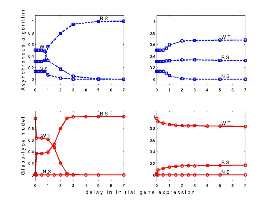
Figure 7: Effect of initially delayed expression in occurrence of steady state patterns. Left: delay in patched expression. Right: delay in cubitus interruptus expression. (results out of 1000 runs).

References

- [1] L. Giot, J. S. Bader, C. Brouwer, A. Chaudhuri, and B. Kuang et al. A protein interaction map of drosophila melanogaster. Science, 302:1727–1736, 2003.
- [2] J. D. Han, N. Bertin, T. Hao, D. S. Goldberg, and G. F. Berriz et al. Evidence for dynamically organized modularity in the yeast protein-protein interaction network. Nature, 430:88–93, 2004.
- [3] S. Li, C. M. Armstrong, N. Bertin, H. Ge, and et al. S. Milstein. A map of the interactome network of the metazoan c. elegans. Science, 303:540–543, 2004.
- [4] T. I. Lee, N. J. Rinaldi, F. Robert, D. T. Odom, and et al. Z. Bar-Joseph. Transcriptional regulatory networks in saccharomyces cerevisiae. Science, 298:799–804, 2002.
- [5] R. Albert. Scale-free networks in cell biology. Journal of cell science, 118:4947–4957, 2005.
- [6] N. M. Luscombe, M. M. Babu, H. Y. Yu, M. Snyder, S. S. Teichmann, and M. Gerstein. Genomic analysis of regulatory network dynamics reveals large topological changes. Nature, 431:308–312, 2004.
- [7] L. Sánchez and D. Thieffry. A logical analysis of the drosophila gap-gene system. J. Theor. Biol., 211:115–141, 2001.
- [8] R. Albert and H. G. Othmer. The topology of the regulatory interactions predicts the expression pattern of the drosophila segment polarity genes. J. Theor. Biol., 223:1–18, 2003.
- [9] L. Mendoza, D. Thieffry, and E. R. Alvarez-Buylla. Genetic control of flower morphogenesis in arabidopsis thaliana: a logical analysis. Bioinformatics, 15:593–606, 1999.
- [10] C. Espinosa-Soto, P Padilla-Longoria, and E. R. Alvarez-Buylla. A gene regulatory network model for cell-fate determination during arabidopsis thaliana flower development that is robust and recovers experimental gene expression profiles. Plant Cell, 16:2923–2939, 2004.
- [11] G. von Dassow, E. Meir, E.M. Munro, and G.M. Odell. The segment polarity network is a robust developmental module. Nature, 406:188–192, 2000.
- [12] M. Chaves, R. Albert, and E.D. Sontag. Robustness and fragility of boolean models for genetic regulatory networks. J. Theor. Biol., 235:431–449, 2005.
- [13] L. Glass. Classification of biological networks by their qualitative dynamics. J. Theor. Biol., 54:85–107, 1975.
- [14] R. Edwards and L. Glass. Combinatorial explosion in model gene networks. Chaos, 10:691–704, 2000.
- [15] L. Glass and S.A. Kauffman. The logical analysis of continuous, nonlinear biochemical control networks. J. Theor. Biol., 39:103–129, 1973.
- [16] J. E. Hooper and M.P. Scott. The molecular genetic basis of positional information in insect segments. In W. Hennig, editor, Early Embryonic Development of Animals, pages 1–49. Springer, Berlin, 1992.
- [17] A. Gallet, C. Angelats, S. Kerridge, and P.P. Thérond. Cubitus interruptus-independent transduction of the hedgehog signal in drosophila. Development, 127:5509–5522, 2000.
- [18] T. Tabata, S. Eaton, and T.B. Kornberg. The drosophila hedgehog gene is expressed specifically in posterior compartment cells and is a target of engrailed regulation. Genes & Dev., 6:2635–2645, 1992.
- [19] K.M. Cadigan, U. Grossniklaus, and W. J. Gehring. Localized expression of sloppy paired protein maintains the polarity of drosophila parasegments. Genes & Dev., 8:899–913, 1994.
- [20] C. Alexandre and J. P. Vincent. Requirements for transcriptional repression and activation by engrailed in drosophila embryos. Development, 130:729–739, 2003.
- [21] D. Swantek and J. P. Gergen. Ftz modulates runt-dependent activation and repression of segment -polarity gene transcription. Development, 131:2281–2290, 2004.
- [22] D.P. Bertsekas and J.N. Tsitsiklis. Parallel and Distributed Computation, Numerical Method. Prentice Hall, Englewood Cliffs, New Jersey, 1989.
- [23] H. de Jong, J.L. Gouzé, C. Hernandez, M. Page, T. Sari, and J. Geiselmann. Qualitative simulation of genetic regulatory networks using piecewise linear models. Bull. Math. Biol., 66:301–340, 2004.
- [24] T. Gedeon. Attractors in continuous-time switching networks. Communications on Pure and Applied Analysis, 2:187–209, 2003.
- [25] A. Mochizuki. An analytical study of the number of steady states in gene regulatory networks. J. Theor. Biol., 236:291–310, 2005.
- [26] N.T. Ingolia. Topology and robustness in the drosophila segment polarity network. PLoS Biology, 2:0805–0815, 2004.