Abstract

It was first suggested by Englander et al to model the nonlinear dynamics of DNA relevant to the transcription process in terms of a chain of coupled pendulums. In a related paper [4] we argued for the advantages of an extension of this approach based on considering a chain of double pendulums with certain characteristics. Here we study a simplified model of this kind, focusing on its general features and nonlinear travelling wave excitations; in particular, we show that some of the degrees of freedom are actually slaved to others, allowing for an effective reduction of the relevant equations.

Introduction and motivation

In a seminal paper appeared a quarter century ago, Englander, Kallenbach, Heeger, Krumhansl and Litwin [12] suggested that DNA solitons, i.e. nonlinear mechanical excitations of the DNA double helix, could have a key role in DNA functional processes – such as DNA transcription and replication – in that they would provide automatic focusing of energy and synchronization of opening along the chain. They also were the first to suggest a simple mechanical model to illustrate their argument; this consisted of a one-dimensional chain of simple pendulums, each of them coupled to the neighboring ones. In this way travelling solitons were described by the sine-Gordon equation, which is known to support both topological and dynamical solitons. (Note that, contrary to the Davydov soliton in alpha-helices [10] which is intrinsically quantum, in this case we deal with classical mechanics and hence classical solitons.)

Following the suggestion of Englander et al., a number of models for the nonlinear dynamics of DNA have been elaborated by different scientists in later years.

Research was pursued essentially in two directions: on the one hand, in DNA denaturation the relevant aspect is the separation between the two helices, and one looks mainly at the degree of freedom describing distance between the two bases in a (Watson-Crick) pair. Considerable progress in this direction has been obtained via the model introduced by Peyrard and Bishop [25]; this has then been refined by Dauxois [9] and extended in the BCP model by Barbi, Cocco and Peyrard [1, 2, 7, 23] (related models are discussed in [21, 35]). See e.g. [3, 24] for a discussion of results and recent advances in this direction, and [8, 26, 30] for matters related to (thermodynamic) stability and bubble formation.

On the other hand, models for the roto-torsional dynamics of DNA have been considered by other authors; the torsional degrees of freedom are relevant in connection with the opening of the DNA double helix taking place to allow RNA-Polymerase to access the base sequence to transcript genetic information [34]. Several models have been proposed in this direction; references and some detail on these can be found in [19, 34].

A particularly simple model (Y model) was proposed by Yakushevich [32, 33]; see also [13, 14, 16, 19]. Despite its simplicity, the Y-model succeeds in describing several relevant features of the DNA nonlinear (and linear) dynamics related to the relevant processes [19, 34, 36], and is thus the subject of continuing interest. In recent works it has been shown that all the (sometimes, very crude) approximations introduced by Yakushevich in her model – some of these substantially affecting the dispersion relations for the model [20] – have very little impact on the fully nonlinear dynamics and in particular on solitons’ shape [17, 18].

The Y model should in any case be seen as only a first step in a hierarchy of increasingly accurate models [33], and has some drawbacks which should be removed by considering more detailed versions of the model; these are both quantitative and conceptual.

On the quantitative side, we mention the impossibility to fit the observed speed of transversal waves in DNA with physical values of the parameters [36]; and the fact that soliton speed remains – provided it is smaller than a maximal speed – essentially a free parameter [15].

On the conceptual side, solitons are possible in these models thanks to the homogeneous character of the chain; but we know that actual DNA is strongly inhomogeneous, as bases are quite different from each other, and homogeneous DNA would not carry any information.

The model we consider here describes the DNA double chain via two (rotational) degrees of freedom per nucleotide, hence it will called a “composite Y model”, following the nomenclature introduced in [4]. These degrees of freedom are related separately to rotation of the sugar-phosphate backbone (which can be of any magnitude) on the one hand, and of the nitrogen bases (which are constrained to a limited range) on the other hand. Both rotations are in the plane perpendicular to the double helix axis.

This model is a simplified – and somehow a “skeleton” – version of the more realistic (and involved) model considered in [4]: in that paper we triggered our model to the actual DNA geometry and dynamics, while here we consider a simplified model so to focus on the general abstract mechanism of interaction between topological and non topological degrees of freedom. For the same reason we will restrict to motions which are symmetric under the exchange of the two chains (as often done also in the analysis of the Peyrard-Bishop and the BCP models).

The model we consider, and more generally the class of composite Y models [4], represents an improvement with respect to the standard Y model both from a quantitative and qualitative point of view.

On the quantitative, phenomenological, side, we have a much higher flexibility of the chain described by the model and dramatic consequences on the model ability to provide realistic physical quantities. E.g., with the composite Y model considered in [4], one obtains the experimentally observed transverse phonon speed using interaction energies of the physical order of magnitude, and a selection of solitons’ speed.

On the qualitative side, which is maybe even more interesting (and more widely applicable than merely DNA), the composite Y model is remarkable in that the uniform and the non-uniform parts of the DNA molecule (backbone and bases respectively) are described by separate degrees of freedom. It happens that, as a consequence of the geometry of the DNA molecule, the degree of freedom describing the backbone supports topological – hence strongly stable – solitons, while the one describing the motion of bases performs quite limited excursion due to steric hindrances; as mentioned above, this is taken into account in our model. It is thus quite conceivable that introducing in the model a non-uniformity which affects only the latter degree of freedom, a perturbation approach would allow to obtain solutions in terms of perturbed solutions for the uniform model; see sections 4 and 5 below.

The perturbative approach is also attractive in that by a suitable limiting procedure, see section 3 below (and [4]), the composite Y model reduces to a standard Y model, for which exact solutions can be obtained. Thus, a perturbative description for the uniform composite Y model can be obtained by perturbing the system near the standard Y solutions.

A drawback of general composite Y models is that the equations describing its dynamics are too complex to be solved analytically, and even the perturbative expansion around the solitonic Y solution can be very hard to control [4]. On the other hand, most of the nice features of the composite model seem to be quite generic, related mostly to doubling of the degrees of freedom and their different topological features, i.e. largely independent of the model details. Numerical investigations for the “realistic” composite Y model of [4] showed that introducing a number of simplifications into the model does not affect its main features – confirming the observations for the standard Y model [17, 18] – but surely makes it easier to handle it at the analytical level.

Motivated by the previous arguments, we study in this paper a simple – possibly the simpler – composite Y model, for which the comparison with the standard Y model is immediate. Our main purpose is indeed to focus on the essential features introduced by having two different kinds of degrees of freedom in chain models.

For the sake of concreteness we make reference to – and discuss the consequences for – DNA dynamics, but it will be quite clear that most of our discussion is more general.

1 The model

Let us now describe our model. We define this in abstract terms, but it can be useful – in order to fix ideas – to recall that in applying it to DNA the “first pendulums” mentioned below and associated to angles $\theta$ represent the nucleosides (segment of the phosphodiester chain and the attached sugar ring), while the “second pendulums” associated to angles $\phi$ represent the nitrogen bases.

We consider two chains of double pendulums. On each chain axis there are equally spaced sites at points of coordinate $z=n\delta$, with $\delta$ a dimensional constant and $n\in{\bf Z}$.

At each site $i\in{\bf Z}$ on each chain axis, there are identical simple ”first pendulums” of length $R$ and mass $M$, which can rotate with no limitations in the plane orthogonal to the axis. The rotation angle of the first pendulum on chain $a=\pm 1$ at site $i$ will be $\theta^{a}_{i}$.

Attached to the point mass of each ”first pendulum” there is a simple ”second pendulum” of length $r$ and mass $m$, which can rotate in the same plane as the first pendulums. The angle of rotation of the second pendulum (with respect to the direction of the first pendulum) will be $\phi^{a}_{i}$. Details are shown pictorially in fig.1.

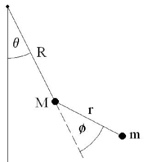
Figure 1: Notation for each of the double pendulums along the two chains; see text.

The second pendulum is not free to swingle through a full circle, but is instead constrained to stay in the range $|\phi^{a}_{i}|\leq\phi_{0}$. This constraint will also be modelled by adding a constraining potential, i.e. a potential $V_{c}(\phi)$ which has the effect of limiting de facto the excursion of the $\phi$ angles.

The reason for this limitation in the $\phi$ range is our intention to model the DNA molecule: in that the bases cannot move outside a certain range, as they would otherwise collide with other parts of the molecule (the phosphodiester chain or the sugar ring).

As for the relative position of the two double pendulums chains, this is such that the distance between the suspension points at the same site – and thus with the same $z$ coordinate – is $2A$. Equivalently, at rest (i.e. for $\theta^{(a)}_{i}=\phi^{(a)}_{i}=0$ for all $a=1,2$ and $i\in{\bf Z}$), the distance between masses at the end of second pendulums at the same site on the two chains is $\ell_{0}:=2(A-R-r)$.

Let us denote, dropping for a moment the index $i$ and writing $a=\pm$ instead of $a=1,2$, as $(x,y)$ the cartesian coordinates – in the plane orthogonal to the double helix axis $z$, with origin in the central point – of the the point mass at the end of the second pendulum.

In the equilibrium position, given by $\theta=\phi=0$, we have $(x,y)=(x_{0},y_{0})$ with $x^{\pm}_{0}=\mp A\pm R\pm r$, $y_{0}=0$. In general,

$$x^{\pm}=\mp A\pm R\cos\theta\pm r\cos(\theta+\phi)\ ,\ \ y^{\pm}=\pm R\sin\theta\pm r\sin(\theta+\phi)\ .$$ (1)

Remark 1. In the standard Yakushevich model, one considers the approximation $\ell_{0}\to 0$; it is known that this approximation has a strong impact on linearized dynamics and dispersion relations [20], but for what concerns fully nonlinear dynamics it has been observed that – at least in the framework of the Yakushevich model – the approximation has a very little impact on travelling solitons [17]. This suggests the possibility of considering the same approximation $\ell_{0}=0$, hence $A=R+r$, here as well. We will indeed adopt this. $\odot$

1.1 The Lagrangian

Let us now describe the different terms appearing in the Lagrangian ${\mathcal{L}}$ for the two chains of double pendulums.

The kinetic energy of the double pendulum (i.e. a disk and the attached pendulum) at site $i$ on chain $a$ is $T^{a}_{i}=(1/2)[I({\dot{\theta}}^{a}_{i})^{2}+m(({\dot{x}}^{a}_{i})^{2}+({\dot{y}}^{a}_{i})^{2})]$; using (1) to express $x^{a}_{i}$ and $y^{a}_{i}$ in terms of $\theta=\theta^{a}_{i}$ and $\phi=\phi^{a}_{i}$, we get with simple algebra

$$T^{a}_{i}\ =\ (I/2){\dot{\theta}}^{2}\,+\,(m/2)\left[R^{2}{\dot{\theta}}^{2}+2Rr\cos\phi\left(({\dot{\theta}})^{2}+{\dot{\theta}}{\dot{\phi}}\right)+r^{2}({\dot{\theta}}+{\dot{\phi}})^{2}\right]\ .$$ (2)

The total kinetic energy is of course $T=\sum_{a,i}T^{a}_{i}$.

We now pass to consider coupling between different double pendulums; we will have only nearest-neighbor interactions, which will be of three different types.

(1) A torsional coupling between successive disks on each chain, described by a potential

$$U_{t}^{(a,i)}\ =\ K_{t}\,[1-\cos(\theta^{a}_{i+1}-\theta^{a}_{i})]\ ;$$ (3)

the total torsional potential is of course $V_{t}=\sum_{a,i}U_{t}^{(a,i)}$. This, albeit entirely natural in terms of the mechanical model (and thus mentioned here), is actually of lesser relevance in modelling DNA and will thus be overlooked; see Remark 3 below.

(2) A stacking coupling between successive pendulums on each chain, described by a potential $U_{s}^{(a,i)}=(1/2)K_{s}[(x^{a}_{i+1}-x^{a}_{i})^{2}+(y^{a}_{i+1}-y^{a}_{i})^{2}]$. This is expressed in terms of the $\theta^{a}_{i}$ and $\phi^{a}_{i}$ angles, using again (1) and with $\lambda=r/R$, as

$$\begin{array}[]{rl}U_{s}^{(a,i)}=&(K_{s}R^{2}/2)\,\left[\left(\cos\theta^{a}_{i}-\cos\theta^{a}_{i+1}+\lambda[\cos(\phi^{a}_{i}+\theta^{a}_{i})-\cos(\phi^{a}_{i+1}+\theta^{a}_{i+1})]\right)^{2}\right.\\ &\left.+\left(\sin\theta^{a}_{i}-\sin\theta^{a}_{i+1}+\lambda[\sin(\phi^{a}_{i}+\theta^{a}_{i})-\sin(\phi^{a}_{i+1}+\theta^{a}_{i+1})]\right)^{2}\right]\ ;\end{array}$$ (4)

the total stacking potential is of course $V_{s}=\sum_{a,i}V_{s}^{(a,i)}$.

(3) A pairing coupling between double pendulums at the same site on opposite chains. We assume this is due to an interaction between the point particles at the extremal points of the pendulums, described by a potential

$$U_{p}^{(i)}\ =\ F(\rho_{i})$$ (5)

where $\rho_{i}$ is the distance between point masses of the two pendulums at site $i$ on the two chains, $\rho_{i}:=[(x_{i}^{(+)}-x_{i}^{(-)})^{2}+(y_{i}^{(+)}-y_{i}^{(-)})^{2}]^{1/2}$. The total pairing potential will of course be $V_{p}=\sum_{i}U_{p}^{(i)}$.

Recent work of ours in the framework of the simple Yakushevich model [17, 18] has shown that the shape of travelling topological solitons is very little affected by the detailed shape of the intrapair potential [18]. We will thus adopt the simplest choice, i.e. an harmonic potential $U_{p}^{(i)}=(1/2)K_{p}\rho_{i}^{2}$; this becomes anharmonic when expressed in terms of the $\theta^{a}_{i}$, $\phi^{a}_{i}$ rotation angles,

$$U_{p}^{(i)}=4K_{p}\left[(R+r)^{2}-rR(1-\cos\phi^{a}_{i})-(r+R)\left(r\cos(\phi^{a}_{i}+\theta^{a}_{i})+R\cos\theta^{a}_{i}\right)\right]\ .$$ (6)

Putting all these together, and considering also the constraining potential $V_{c}$ to be discussed below, the Lagrangian describing our system will therefore be

$${\mathcal{L}}\ =\ T\ -\ \left(V_{t}+V_{s}+V_{p}+V_{c}\right)\ .$$ (7)

Some remarks are in order concerning the potential interactions introduced above.

Remark 2. We have explicitly assumed harmonic potentials for the torsional and stacking coupling between successive elements (disks and pendulums respectively) on the same chain. It should be mentioned, in this context, that recent work by Saccomandi and Sgura has shown that the choice of a harmonic potential for the interpair interactions (torsional and stacking couplings) is not without effect: considering non-harmonic couplings leads to a stronger energy localization [28]. We will defer consideration of the effect of anharmonic interpair couplings in our model to later work. $\odot$

Remark 3. We also note that we have considered here both a torsional coupling originating in the coupling between adjacent first pendulums (in DNA, in the phosphodiester chain) and a rotational interaction originating in interaction between adjacent second pendulums (in DNA this models the stacking interaction between neighboring bases).

The physical origin of these in actual DNA molecule is rather diverse. Indeed, the stacking interaction is essentially due to polar interaction between the bases; these are essentially flat and rigid assemblies of atoms with a strong dipolar momentum, and correspondingly we have (in physico-chemical notation) a $\pi-\pi$ bond. On the other hand, the segment of a hypothetical phosphodiester chain without attached bases would be essentially free to rotate with respect to each other (if not for rather small polar forces), the main obstacle to such motion originating in hindrances caused by bases and their occupied volume and polar moments.

It is thus reasonable, as announced above (and also in view of the considerable complications of equations that would be obtained from the full Lagrangian and the fact the two motions are strongly related geometrically), to consider the approximation $K_{t}\to 0$, as we do from now on. This corresponds to the well known fact that the forces stabilizing the DNA double chain are essentially the interbase pairing interaction and the stacking interaction [24], i.e. those corresponding to our terms $V_{p}$ and $V_{s}$. $\odot$

Remark 4. Further support to this kind of approximation comes from the results of [4], where the model with non vanishing torsional interaction has been investigated in detail. In that case, the torsional energy is a full order of magnitude lesser then the stacking energy. Moreover, numerical soliton solutions studied in that context showed that the form of the soliton remains almost the same if $K_{t}=0$ and all the torsional potential energy is transferred on the stacking term (see the Fig. 8 of [4]). $\odot$

Remark 5. We stress that, as quite common in DNA mechanical models, we are dealing with the DNA molecule per se, i.e. we do not consider interactions of the double chain with the solvent (the fluid environment it is immersed in). This interaction would lead to exchange of energy with the solvent, with dissipation and random terms appearing in our dynamical equations (some authors have taken into account interaction with the solvent by introducing correction terms in the intrapair potential $V_{p}$ [37, 38]). We hope a model modified in this direction can be studied in the near future. $\odot$

1.2 Constraints and constraining potential

It should be recalled that the angles $\theta$ and $\phi$ are not on the same footing. Indeed, while $\theta$ is free to take any value, $\theta\in{\bf R}$, the angle $\phi$ is constrained to be in the range

$$\phi\ \in\ [-\phi_{0},\phi_{0}]\ .$$ (8)

The Euler-Lagrange equations (see below) for the Lagrangian (7) should be complemented with such a constraint.

Note that (8) is an anholonomic constraint, and taking it into account is somehow inconvenient. It may be convenient, in particular in numerical computations, to remove the constraint and introduce instead a constraining potential. That is, we allow in principles $\phi$ to take any value, but introduce a potential $U_{c}(\phi)$ which makes very costly energetically any value of $\phi$ outside the range specified in (8), and has an irrelevant effect on the dynamics when $\phi$ is within this range.

Any expression for the potential $U_{c}$ would be acceptable, provided $U_{c}$ is essentially flat for $|\phi|<\phi_{0}$ and rises sharply as soon as we approach the border – or are outside – of this range. A convenient form for $U_{c}$ is

$$U_{c}(\phi)\ =\ \exp[(K_{c}/2)(\phi^{2}-\phi_{0}^{2})]$$ (9)

with $K_{c}>>1$. The total constraining potential appearing in the Lagrangian will then of course be

$$V_{c}\ =\ \sum_{a}\sum_{i}U_{c}(\phi^{(a)}_{i})\ .$$ (10)

1.3 Equations of motion

The equations of motion for the model are the Euler-Lagrange equations for the Lagrangian (7). These are obtained with standard algebra, and are relatively involved expressions, which we do not write explicitly. The equation for the dynamics of variables associated with site $i$ involve also values of variables at neighboring sites $i\pm 1$.

We are mainly interested in solutions which vary slowly in space on the space scale set by the intersite distance $\delta$. It is thus convenient to pass to the continuum approximation; this means promoting the array of values $\phi^{a}_{i}(t)$ to a field variable $\Phi^{a}(z,t)$ such that $\Phi^{a}(n\delta,t)=\phi^{a}_{n}(t)$, and similarly promoting $\theta^{a}_{i}(t)$ to a field variable $\Theta^{a}(z,t)$ such that $\Theta^{a}(n\delta,t)=\theta^{a}_{n}(t)$. (Note we are keeping the dimensional constant $\delta$, so to have physical units – rather chain units – for $z$.)

Moreover, in order to focus on the essential features of the model – and similarly to what is traditionally done in studying the Peyrard-Bishop and Barbi-Cocco-Peyrard models [1, 2, 24, 25] – we will just consider symmetric motions; that is, we assume $\phi^{(+)}_{i}(t)=\phi^{(-)}_{i}(t)$, $\theta^{(+)}_{i}(t)=\theta^{(-)}_{i}(t)$ which of course entails equality of the field variables as well. We will thus write simply $\Phi^{(\pm)}(z,t)=\Phi(z,t)$, $\Theta^{(\pm)}(z,t)=\Theta(z,t)$; and similarly for derivatives.

Remark 6. It should be stressed that if we restrict to symmetric solutions in discussing the standard Y model, then only one type of kink solitons can exist, i.e. those connecting equilibrium positions at $x=\pm\infty$ with a total phase shift of $\pm 2\pi$; higher solitons, even if with symmetric topological numbers, would require a deviation from a fully symmetric dynamics. $\odot$

In this setting, we write $\phi_{i}\simeq\Phi$ and $\theta_{i}\simeq\Theta$ for variables at site $i$; and for neighboring sites we have, expanding in Taylor series up to order two in $\delta$,

$$\phi_{i\pm 1}=\Phi\pm\delta\Phi_{z}+(1/2)\delta^{2}\Phi_{zz}\ \ ,\ \ \ \theta_{i\pm 1}=\Theta\pm\delta\Theta_{z}+(1/2)\delta^{2}\Theta_{zz}\ .$$ (11)

With these, the Euler-Lagrange equations issued from (7) are rewritten as second order PDEs for $\Phi$ and $\Theta$. In order to simplify the writing, we introduce the notations

$$\alpha(\Phi)\ :=r^{2}+rR\cos(\Phi)\ ;\ \ \beta(\Phi)\ :=\ r^{2}+R^{2}+2rR\cos(\Phi)\ .$$ (12)

The Euler-Lagrange equations are then given explicitly by

$$\begin{array}[]{l}\delta^{2}K_{s}(r^{2}+rR\cos\Phi)\,\Phi_{xx}\ +\ \delta^{2}K_{s}(r^{2}+R^{2}+2rR\cos\Phi)\,\Theta_{xx}\ +\\ \ \ -\ [MR^{2}+m(r^{2}+R^{2}+2rR\cos\Phi)]\,\Theta_{tt}\ -\ m(r^{2}+rR\cos\Phi)\,\Phi_{tt}\ =\\ \ \ \ =\ rR[(\delta^{2}K_{s}\sin\Phi)\Phi_{x}(\Phi_{x}+2\Theta_{x})\ -\ (m\Phi_{t}(\Phi_{t}+2\Theta_{t})]\ +\\ \ \ \ +\ 4K_{p}(rR+R^{2})\sin\Theta\ +\ 4K_{p}(rR+r^{2})\sin(\Phi+\Theta)\ ;\\ \delta^{2}K_{s}r^{2}\,\Phi_{xx}\ +\ \delta^{2}K_{s}(r^{2}+rR\cos\Phi)\,\Theta_{xx}\ +\\ \ \ -\ mr^{2}\,\Phi_{tt}\ -\ m(r^{2}+rR\cos\Phi)\,\Theta_{tt}\ =\\ \ \ \ =\ -\ (rR\sin\Phi)(4K_{p}-m\Theta_{t}^{2}+\delta^{2}K_{s}\Theta_{x}^{2})\ +\\ \ \ \ +\ 4K_{p}r(r+R)\sin(\Phi+\Theta)\ +\ K_{c}\,\exp[(K_{2}/2)(\Phi^{2}-\phi_{0}^{2})]\,\Phi\end{array}$$ (13)

2 Travelling wave solutions (solitons)

We are specially interested in travelling wave solutions, i.e. solutions satisfying

$$\Phi(z,t)\,=\,\varphi(z-vt)\,\equiv\,\varphi(\xi)\ ,\ \ \Theta(z,t)\,=\,\vartheta(z-vt)\,\equiv\,\vartheta(\xi)\ .$$ (14)

These will be called “solitons” – provided they satisfy suitable boundary conditions, see below – following the common language in DNA modelling, and are indexed by an integer (i.e. a topological winding number). We stress that they are not proven to be dynamical solitons in the rigorous mathematical sense [6]; on the other hand, they are topological solitons in the sense of field theory [11].

2.1 Equations of motion

With this ansatz, the equations (13) read

$$\begin{array}[]{l}\mu(r^{2}+rR\cos\phi)\ \phi^{\prime\prime}\ +\ (J+2\mu rR\cos\phi)\ \theta^{\prime\prime}\ =\\ \ \ \ \mu(rR\sin\phi)\,[(\phi^{\prime})^{2}+2\phi^{\prime}\theta^{\prime}]\ -\ 4K_{p}[(rR+R^{2})\sin\theta\,+\,(rR+r^{2})\sin(\phi+\theta)]\ ;\\ \mu r^{2}\,\phi^{\prime\prime}\ +\ \mu(r^{2}+rR\cos\phi)\,\theta^{\prime\prime}\ =\ (4K_{p}rR+\mu rR(\theta^{\prime})^{2})\,\sin\phi\ +\\ \ \ \ -\ 4K_{p}r(r+R)\,\sin(\phi+\theta)\ +\ K_{c}\,\exp[(K_{c}/2)(\phi^{2}-\phi_{0}^{2})]\,\phi\ .\end{array}$$ (15)

Here we have simplified the writing by introducing the parameters

$$\mu\ :=\ m\,v^{2}\ -\ K_{s}\,\delta^{2}\ ,\ \ J\ =\ (\mu(r^{2}+R^{2})+MR^{2}v^{2})\ .$$ (16)

In the analysis of the (15), we will proceed perturbatively; see next section.

2.2 Finite energy condition and boundary conditions

The equations (15) are a reduction of (13), which are in turn issued by the Lagrangian (7). The latter is well defined on fields $\Phi(z,t),\Theta(z,t)$ satisfying a finite energy condition; in the continuum approximation the action $S$ is given by integration over $z\in(-\infty,+\infty)$ of the Lagrangian density obtained as the continuum limit of (7). In the present case, where we have a kinetic and a potential energy parts, the finite energy condition corresponds to requiring that for large $|z|$ the kinetic energy vanishes and the configuration correspond to points of minimum for the potential energy.

By the explicit expression of the kinetic energy and of our potentials, this means

$$\begin{array}[]{l}\Phi(\pm\infty,t)=0\ ,\ \Theta(\pm\infty,t)=2n_{\pm}\pi\ ,\\ \Phi_{z}(\pm\infty,t)=0\ ,\ \Theta_{z}(\pm\infty,t)=0\ ,\\ \Phi_{t}(\pm\infty,t)=0\ ,\ \Theta_{t}(\pm\infty,t)=0\ ;\end{array}$$ (17)

where of course $\Phi(\pm\infty,t)$ stands for $\lim_{z\to\pm\infty}\Phi(z,t)$, and so on.

When we pass to the travelling waves equation, this means that we must impose on the functions $\varphi(\xi)$, $\vartheta(\xi)$ the boundary conditions

$$\varphi(\pm\infty)=0\ ,\ \vartheta(\pm\infty)=2n_{\pm}\pi\ ,\ \ \varphi^{\prime}(\pm\infty)=0\ ,\ \vartheta^{\prime}(\pm\infty)=0\ .$$ (18)

In the following we will describe the dynamics of $\vartheta(\xi),\varphi(\xi)$ in terms of motions (in the fictitious time $\xi$) in an effective potential; note that such a motion can satisfy the boundary conditions (18) only if $(\varphi,\vartheta)=(0,2\pi k)$ is a point of maximum for the effective potential. The solutions satisfying (18) can hence be classified by the winding number $n:=n_{+}-n_{-}$.

In the following we will in particular attempt to describe the basic ($n=1$) soliton; note that – as stressed in Remark 6 – this is the only case for which we can fully compare the solutions of our model with those of the standard Y model within the frame of symmetric solutions.

3 Perturbative expansion around Yakushevich solitons

As remarked above, while ($\theta$ and hence $\Theta$ and) $\vartheta$ can take any value, the range of ($|\phi|$ and hence $|\Phi|$ and) $|\varphi|$ is limited by $\phi_{0}$; thus if $\phi_{0}=\varepsilon<<1$, we are guaranteed $\varphi$ will also be of order $\varepsilon$.

On the other hand, for $\phi_{0}\to 0$ and hence $\varphi\to 0$, the $\phi$ degree of freedom is frozen and we are effectively back to consider the Y model [4]; we would then obtain the soliton solutions to our model as a perturbation of the corresponding soliton solutions for the Y model. The Y model can be also recovered from our composite model by acting on the geometrical parameter characterizing it [4]; this essentially amounts to a suitable limit $r=0$. Here “suitable” means that some care should be taken in the rescaling in order to avoid a singular limit arises.

We want to study the equations of motion for our model in the regime of small $\varepsilon$, by looking at them as a perturbation of the standard Yakushevich equations. We stress that we are considering the symmetric (in the chain exchange) setting, and adopting the contact approximation $A=R+r$.

We will take $\phi_{0}=\varepsilon<<1$ and expand in $\varepsilon$. We will also take $r=\varepsilon r_{0}$ and, in order to keep the total length of the double pendulum $A=R+r$ constant, $R=A-\varepsilon r_{0}$.

Remark 7. As shown in [17], one can obtain analytic results also without letting $\ell_{0}\to 0$; on the other hand it is also shown there that a nonzero $\ell_{0}$ does actually produce a very small modification in the solitons’ shape, but yields much more involved analytic formulas. Thus, in the present context it is convenient to adopt $\ell_{0}=0$. Note that in any case we should keep the physical distance $A$ fixed as $\varepsilon$ is varied. $\odot$

We will expand $\varphi$ and $\vartheta$ to order $\varepsilon$. We write

$$\begin{array}[]{l}\varphi=\psi+\varepsilon\varphi_{0}\ +O(\varepsilon^{2})\ ,\\ \vartheta=\vartheta_{0}+\varepsilon\eta\ +O(\varepsilon^{2})\ .\end{array}$$ (19)

We plug this into equation (15) and expand the equations so obtained to first order in $\varepsilon$, obtaining the equations

$$\begin{array}[]{l}A^{2}((\mu-Mv^{2}){\vartheta_{0}}^{\prime\prime}-4K_{p}\sin\vartheta_{0})+A\left[-(\mu-Mv^{2})(2r_{0}{\vartheta_{0}}^{\prime\prime}-A\eta^{\prime\prime})+\right.\\ \ \ \ \left.+r_{0}(\psi^{\prime\prime}+2\mu{\vartheta_{0}}^{\prime\prime})\cos\psi-\psi^{\prime}r_{0}(\psi^{\prime}+2{\vartheta_{0}}^{\prime})\mu\sin\psi-4K_{p}r_{0}\sin\vartheta_{0}+\right.\\ \ \ \ \left.-4K_{p}(A\eta\cos\vartheta_{0}-2r_{0}\sin\vartheta_{0})-4K_{p}r_{0}\sin(\psi+\vartheta_{0})\right]\varepsilon\ =\ 0;\\ -\exp[(K_{c}/2)\psi^{2}]K_{c}\psi\ +\ \left[A\mu r_{0}(\cos\psi){\vartheta_{0}}^{\prime\prime}+Ar_{0}(4K_{p}+\mu({\vartheta_{0}}^{\prime})^{2})\sin\psi+\right.\\ \ \ \ \left.-4AK_{p}r_{0}\sin(\psi+\vartheta_{0})-\exp[(K_{c}/2)\psi^{2}]K_{c}(1+K_{c}\psi^{2})\varphi_{0}\right]\varepsilon\ =\ 0\ .\end{array}$$ (20)

At order zero the second equation in (20) yields simply

$$\psi\ =\ 0\ .$$ (21)

With this, the equations (20) become quite simpler, i.e. reduce to

$$\begin{array}[]{l}A^{2}((\mu-Mv^{2}){\vartheta_{0}}^{\prime\prime}-4K_{p}\sin\vartheta_{0})+\\ \ \ \ +A\left[2Mr_{0}v^{2}{\vartheta_{0}}^{\prime\prime}+A(\mu-Mv^{2})\eta^{\prime\prime}-4A\eta K_{p}\cos\vartheta_{0}\right]\ \varepsilon\ =0\ ;\\ \left[-K_{c}\varphi_{0}+A\mu r_{0}{\vartheta_{0}}^{\prime\prime}-4AK_{p}r_{0}\sin\vartheta_{0}\right]\ \varepsilon\ =\ 0\ .\end{array}$$ (22)

We will now compute the leading term contributions for $\vartheta$ and for $\varphi$; this will suffice to show our main point, emphasized in section 4. See Appendix B for the $O(\varepsilon)$ correction to $\vartheta$.

3.1 The leading term for $\vartheta$

As for the first of (22), at order zero we get a sine-Gordon equation,

$${\vartheta_{0}}^{\prime\prime}\ =\ -(4K_{p}R^{2}/J)\ \sin\vartheta_{0}\ .$$ (23)

This can be seen as describing the motion (in the fictitious time $\xi$) of a point particle of unit mass in the field of an effective potential

$$V_{0}\ =\ {4K_{p}R^{2}\over J}\ (1-\cos\vartheta_{0})\ ,$$ (24)

where the additive constant has been chosen so that for $\vartheta_{0}=0$ we get $V_{0}=0$.

It is important to stress that the leading term of the perturbative expansion reproduces the Y soliton equation (23) without any further constraint. In particular there is no constraint on the travelling speed of the soliton.

Remark 8. This behavior should be compared with that described in [4] for a similar model, which differs from that under consideration here, essentially for the presence of a non vanishing torsional potential. In this latter case setting $\varphi=0$ allows to recover the Y soliton but the speed of the travelling wave is fixed in terms of the torsional constant $K_{t}$; moreover, the solitonic solution exists only when $K_{t}/I<K_{s}/m$ [4]. The fact that the above constraints disappear when $K_{t}=0$ sheds light on the physical meaning of the result of [4]: the constraint fixing the soliton speed found in [4] has a purely dynamical origin and is completely independent from both the geometry and the doubling of the degrees of freedom introduced in the composite model; its origin has to be traced back to the interplay between torsional and stacking potential energy which characterizes the composite Y model analyzed in [4]. $\odot$

As discussed above, the boundary conditions (18) require that $\vartheta_{0}=0$ corresponds to a maximum for the effective potential; it is apparent from (24) that this is the case if and only if $J<0$, which we assume from now on. By the expression of $J$, see (16), this is the case provided

$$v^{2}\ <\ K_{s}\delta^{2}\ {r^{2}+R^{2}\over(M+m)R^{2}+mr^{2}}$$ (25)

(the limiting speed for the standard Y model is recovered for $r\to 0$). It should be noted that for $v$ satisfying (25), the parameter $\mu$ is also negative, $\mu<0$ (more precisely, $-K_{s}\delta^{2}<\mu<-K_{s}\delta^{2}(1+(m/M)(1+(r/R)^{2}))^{-1}$.)

The “conservation of energy” in the potential $V_{0}$ for motions satisfying (18) reads $(1/2)(\vartheta_{0}^{\prime})^{2}+V_{0}(\vartheta_{0})=0$, i.e. we get ${\vartheta_{0}}^{\prime}=4R\sqrt{(K_{p}/|J|)}\,\sin(\vartheta_{0}/2)$. The equation is integrated explicitly by separation of variables, yielding

$$\left[\log\left(\tan(\vartheta_{0}/4)\right)\right]\ =\ K(\xi-\xi_{0})\ ,$$ (26)

where we have defined $K:=2R\sqrt{K_{p}/|J|}$; note that choosing $\xi_{0}=0$ corresponds to requiring that $\vartheta_{0}(0)=\pi$. With this, and inverting (26), we have the solution (plotted in fig.2.a)

$$\vartheta_{0}(\xi)\ =\ 4\ {\rm arctan}\left[\exp\left(K\xi\right)\right]\ .$$ (27)

(a)	(b)

Figure 2: Left (a): the function $\vartheta_{0}(\xi)$, see (27). Right (b): the function $\varphi_{0}(\xi)$, see (29). Here we adopted the parameter values discussed in Appendix A, and plotted the case $v=0$; we also used $K_{c}=30$ in (b). The distance along DNA axis $\xi$ is measured in units of the intersite distance $\delta$, and $\vartheta_{0}$, $\varphi_{0}$ in units of $\pi$.

3.2 The leading term for $\varphi$

Let us now pass to consider the $O(\varepsilon)$ terms in (22). In particular, the second equation reads

$$K_{c}\varphi_{0}+2qR(4K_{p}\sin\vartheta_{0}+\mu{\vartheta_{0}}^{\prime\prime})$$ (28)

and yields directly an expression for $\varphi_{1}$ in terms of $\vartheta_{0}$. Using the equation (23), this is

$$\varphi_{0}\ =\ -{8K_{p}qR(\mu R^{2}-J)\over JK_{c}}\ \sin\vartheta_{0}\ .$$ (29)

This function is plotted in fig.2.b.

4 Slaved fields and realistic DNA modelling

We have thus obtained the first order term of the $\varepsilon$ expansion for $\varphi$ in terms of the $\vartheta_{0}$ solution, with an algebraic rather than differential equation, see (29). In other words, $\varphi_{0}$ is slaved to $\vartheta_{0}$; the same could be said more generally for the field $\Phi$ with respect to the field $\Theta$.

It is quite apparent that this feature is due to the different nature of the fields in our model. As already pointed out, $\Theta$ is free to change and go round the circle (is topological), while $\Phi$ is constrained to small variations. When we look for finite energy solutions, moreover, $\Theta$ will join different vacua at $z=\pm\infty$, while $\Phi$ can at most have small oscillations around the zero value.

If we look at this feature from the point of view of DNA modelling, one point should be stressed. That is, suppose we had a non-homogeneous model, the inhomogeneity being however such to affect only the dynamical parameters related to the interaction between $\phi_{i}$ angles. In this case, the constants appearing in (29) would not be constant any more, and actually depend on the $z$ coordinate – in the travelling wave reduction, on $\xi$ and also on the parameter $v$ describing the speed of the travelling wave. This would lead to a more involved expression for $\varphi_{0}$ in terms of $\vartheta_{0}$, now depending explicitly on $\xi$ as well as on $v$, and with all parameters being a function of $\xi$; but the relevant point is that we would still be able to express $\varphi_{0}$ in terms of $\vartheta_{0}$.

Needless to say, this is only true at first order, and higher order computations would soon become very much involved. On the other hand, it remains true that the “master” dynamics would be the one related to the $\theta$ angles, and the $\phi$ angles would remain slaved at all orders; that is, writing

$$\vartheta=\vartheta_{0}+\varepsilon\sum_{k=0}^{\infty}\varepsilon^{k}\eta_{k}\ ,\ \varphi=\sum_{k=0}^{\infty}\varepsilon^{k}\psi_{k}\ ,$$

the equation for $\eta^{k}$ would depend on $\psi_{0},...,\psi_{k-1}$ (beside depending of course on $\vartheta_{0}$ and on $\eta_{1},...,\eta_{k-1}$), while $\psi_{k}$ would be determined algebraically by $(\vartheta_{0},\eta_{1},...,\eta_{k-1})$ in the $\varphi$ expansion.

The separation of the degrees of freedom in “master” and “slaves” is related to a nonperturbative feature of the dynamical system (15). The first integral of Eqs. 15) can be written in the form $\varphi^{\prime}=F(\theta^{\prime},\theta,\varphi,E)$ where $E$ is an integration constant ( the energy). Eliminating $\varphi^{\prime\prime}$ from the system (15) and using the first integral above, one can always write the resulting equation in the form $G(\theta^{\prime\prime},\theta^{\prime},\theta,\varphi,E)=0$, which defines in implicit form $\varphi$ as a function of $(\theta^{\prime\prime},\theta^{\prime},\theta,E)$. Thus, once a (perturbative or non perturbative) solution for $\theta$ is known, the corresponding expression for $\varphi$ can be obtained algebraically.

5 Discussion

We have considered a mechanical model consisting of two chains of double pendulums, coupled with each other at each chain site. This “skeleton” model is the simpler specimen of a class of models for DNA roto-torsion dynamics which is aimed at improving the Yakushevich model, within the approach set forth by Englander et al. [12], and should show the essential characteristics for the class keeping to a minimum the unessential mathematical complications.

An element of this class – based on a geometrically more complex and realistic description of the internal structure of DNA – has been considered in [4]. We have introduced two simplifications with respect to that model, which have been suggested by numerical results for that model itself: bases have been considered as point particles, and torsional interaction disregarded. These two quite reasonable approximations simplify drastically the dynamics of the system.

We have determined the PDEs describing the motions in the long wavelength approximation, and also the reduction to travelling wave solutions. The finite energy condition imposes boundary conditions such that the finite energy solutions can be classified by a topological integer – actually a winding number for the field $\Theta$ and hence for $\vartheta$ – and minimal energy solutions in each topological sector are topological solitons.

The equation of motion describing travelling waves for our skeleton model are simple enough so that a (first order) perturbative expansion around the well known Yakushevich soliton can be used to find approximate analytical solutions.

It seems appropriate to point out some drawbacks of our discussion.

(A) The question if our model equations support dynamical solitons in rigorous mathematical sense [6] was not solved nor tackled.

(B) Similarly, we did not investigate the convergence of the perturbation expansion around Y solitons, and just considered first orders contributions.

(C) Also, as mentioned in Remark 5 and relevant for DNA modelling, we did not consider interactions of the double chain with the solvent.

On the other hand, we provided a simple model for a nonlinear (double) chain showing some features which – in our opinion – are quite interesting both per se (i.e. in the frame of nonlinear dynamics for discrete systems) and for applications, in particular to DNA roto-torsional dynamics.

In particular, the model is simple enough to allow for an explicit analysis, yet displays a very interesting interaction of topological and non-topological degrees of freedom.

We have shown that the equations can be tackled in terms of a perturbation expansion around the Yakushevich soliton, and computed the behavior of the new (non-topological) field at first order. Quite remarkably, this is completely determined by the behavior of the topological field at order zero. That is (in fluid dynamics language), the field $\Phi$ appears to be slaved to the field $\Theta$.

Appendix A. Parameters for DNA modelling

Our model Lagrangian (7) depends on several parameters. Whatever the interest of the model per se, and albeit we conducted our discussion in general terms, we are primarily motivated by its application to describe the nonlinear dynamics of DNA; hence we are interested in the values of these parameters for the physical situation (also to be used in numerical plots later on).

We will not discuss the derivation of these, referring to [5, 24, 29, 31, 34] as well as to the detailed discussion given in [4].

As for the geometrical parameters, the physical values are

$$A\simeq 10.5\AA\ ,\ R\simeq 6.0\AA\ ,\ r\simeq 3.0\AA\ .$$

Note that $\ell_{0}=2(A-R-r)$ is the length of the pairing H-bonds at equilibrium; we have $\ell_{0}\simeq 3.0\AA$, in agreement with the physical situation [31].

In our discussion of the model, we have chosen to adopt Yakushevich contact approximation $\ell_{0}=0$, which entails $A=R+r$. We choose then to rescale $A$ by a factor (5/6), so to satisfy this. Note that as our formulas only involve $r$ and $R$, and not $A$, this does not show up in there.

The dynamic parameters are the effective masses $M$ and $m$; their values are related with the moments of inertia $I_{s}$ and $I_{b}$ for the rotations considered in the model. For these moments of inertia we adopt the values [4] $I_{s}\simeq 2\cdot 10^{-22}\,{\rm g\AA}^{2}$ and $I_{b}\simeq 5.5\cdot 10^{-21}\,{\rm g\AA}^{2}$, which yields for the effective masses the values

$$M=I_{s}/R^{2}=5.5\cdot 10^{-20}\,{\rm g}\ ,\ \ m=I_{b}/r^{2}\simeq 6.0\cdot 10^{-20}\,{\rm g}\ .$$

Finally, for the coupling constants we adopt (see again the discussion in [4]) the values

$$K_{p}\ \simeq\ 0.022{\rm eV/\AA}^{2}\ ,\ K_{p}r^{2}\simeq 0.2{\rm eV}\ ,\ K_{s}\ \simeq\ 0.25{\rm eV}\ .$$

These values were used in the numerical computations and in the plots of solution solutions given in the main text.

In particular, with these values of the physical parameters and for $v=0$, the parameters $K=2R\sqrt{K_{p}/|J|}$ controlling the soliton’s shape, and $\alpha$ appearing in (B.1) below take the value

$$K\ \simeq\ 0.53\ ;\ \ \alpha\ \simeq\ 0.35\ .$$

Appendix B. Order $\varepsilon$ corrections for $\vartheta$

In the main text we provided the leading order terms for the solution to (22), i.e. a solution at order $\varepsilon^{0}$ for $\vartheta$, and at order $\varepsilon$ for $\varphi$; it is appropriate to mention that the $O(\varepsilon)$ correction to the $\vartheta$ computed above, call it $\varepsilon\eta$, can be explicitly computed.

Indeed the $O(\varepsilon)$ terms in the first of (22) provides, using (27),

$$\eta^{\prime\prime}\ =\ -\ \alpha\,\cos\vartheta_{0}\ \eta\ -\ \beta\,\sin\vartheta_{0}\ ;$$

we have written, for ease of notation,

$$\alpha\,=\,{4K_{p}/(\mu+Mv^{2})}\ ,\ \beta\,=\,{8K_{p}Mr_{0}v^{2}/[A(\mu+Mv^{2})^{2}]}\ .$$

We were not able to solve the equation (B.1) in general; however, if we look at the case $v\to 0$, then $\beta\to 0$ and the equation reduces to

$$\eta^{\prime\prime}\ =\ -\ {4K_{p}\over\mu}\,\cos\vartheta_{0}\ \eta\ .$$

It is convenient to express $\eta(\xi)$ as a function $\rho(\vartheta_{0})$ of $\vartheta_{0}$ (which is a monotone function of $\xi$, as seen above); with this, and with some simple algebra, the equation (B.2) reads

$$2(1-\cos\vartheta_{0})\,\rho^{\prime\prime}\ -\ (\sin\vartheta_{0})\,\rho^{\prime}\ +\ (\cos\vartheta_{0})\,\rho\ =\ 0\ .$$

Note that we should as well require that $\rho(0)=0=\rho(2\pi)$, as the boundary conditions are satisfied by the first order contribution $\vartheta_{0}$.

The solutions to (B.3) satisfying the boundary conditions are given in terms of the hypergeometric function ${}_{2}F_{1}$ by

$$\rho(\vartheta_{0})\ =\ \sqrt{(1-\cos\vartheta_{0})}\ \ {}_{2}F_{1}\left({1-i\sqrt{7}\over 4},{1+i\sqrt{7}\over 4},1,{1\over 2}(1-\cos\vartheta_{0})\right)\ ;$$

this is readily converted into $\eta(\xi)$ using (27) and recalling that

$$\eta(\xi)\ :=\ \rho[\vartheta_{0}(\xi)]\ .$$

Note it follows from (27) and trigonometric manipulations that

$$\cos(\vartheta_{0})\ =\ {1-6x^{2}+x^{4}\over(1+x^{2})^{2}}\ ,\ \ {\rm where}\ x:=\exp[K\xi]\ .$$

As for the stability of this solutions, it follows from our selection of the function space to which solutions must belong, i.e. from the boundary conditions at $\pm\infty$. In fact, we note that as $\vartheta_{0}(\xi)$ already satisfies the appropriate limit conditions for $\xi\to\pm\infty$, the correction $\eta(\xi)$ should vanish for $\xi\to\pm\infty$; this implies the stability of the solution.

The behavior of solutions for large $|\xi|$ can also be considered as follows. For $\xi\to\pm\infty$ the term $\cos(\vartheta_{0})$ goes to 1, and asymptotically in $\xi$ eq.(B.2) reduces to

$$\eta^{\prime\prime}\ =\ {4K_{p}\over|\mu|}\ \eta\ ,$$

where we have used $\mu<0$; needless to say, the solution of this is given (in the $\xi\to\pm\infty$ region) by

$$\eta\ =\ A_{\pm}\sinh(2\sqrt{K_{p}/|\mu|}\xi)\,+\,B_{\pm}\cosh(2\sqrt{K_{p}/|\mu|}\xi)\ .$$

The limit conditions require that $A_{\pm}=\pm B_{\pm}$.

Appendix C. Perturbative expansion for general solutions

We have considered expansion around Yakushevich soliton within the function space ${\mathcal{F}}$ identified by the boundary conditions (2.4) and by the travelling wave ansatz (2.1). It is of course possible to consider expansion around the Yakushevich soliton $\vartheta_{0}(x-vt)$ also for functions which are in ${\mathcal{F}}$ but are not necessarily travelling waves. In this case the expansion (3.1) is replaced by (we could as well insert a term $\Psi(x,t)$ of order one in $\Phi(x,t)$; the vanishing of it would however obviously result from the equations obtained at order $\varepsilon^{0}$)

$$\begin{array}[]{l}\Phi(x,t)\ =\ \varepsilon\,\phi(x,t)\,+\,O(\varepsilon^{2})\ ,\\ \Theta(x,t)\ =\ \vartheta_{0}(x-vt)\,+\,\varepsilon\,\eta(x,t)\,+\,O(\varepsilon^{2})\ .\end{array}$$

Note that (2.4) imply that the perturbation fields $\phi(x,t)$ and $\eta(x,t)$ must vanish for $x\to\pm\infty$.

Inserting the (C.1) into the Euler-Lagrange equations (1.13) we obtain at order $\varepsilon$ two equations. One of these is actually an algebraic relation between $\phi$ and $\vartheta_{0}$, which reads explicitly

$$\phi\ =\ -\ {4AK_{p}Mr_{0}v^{2}\over K_{c}((M+m)v^{2}-K_{s}\delta^{2})}\ \sin(\vartheta_{0})\ .$$

We stress that this imply that the $\Phi$ field is slaved, even without the restriction to travelling waves.

As for the other $O(\varepsilon)$ equation, this reads

$$(K_{s}\delta^{2})\,\eta_{xx}\,-\,(M+m)\,\eta_{tt}\ =\ 4K_{p}\,\cos(\vartheta_{0})\,\eta\,+\,8{K_{p}Mr_{0}v^{2}\over A((M+m)v^{2}-K_{s}\delta^{2})}\,\sin(\vartheta_{0})\ .$$

Here and above we have used the writing $\sin(\vartheta_{0})$, $\cos(\vartheta_{0})$ albeit these are known functions of $\xi=(x-vt)$, see (B.6), for ease of writing.

For large $|t|$ and finite $x$ the (C.3) reduces to the autonomous equation

$$(K_{s}\delta^{2})\,\eta_{xx}\,-\,(M+m)\,\eta_{tt}\ =\ 4K_{p}\,\cos(\vartheta_{0})\,\eta\ ;$$

the dispersion relations for this are easily obtained setting $\eta(x,t)=f_{k\omega}\exp[i(qx-\omega t)]$ and are given by

$$\omega\ =\ \pm\sqrt{{4K_{p}+K_{s}\delta^{2}q^{2}\over M+m}}\ .$$

References

- [1] M. Barbi, S. Cocco and M. Peyrard, “Helicoidal model for DNA opening”, Phys. Lett. A 253 (1999), 358-369
- [2] M. Barbi, S. Cocco, M. Peyrard and S. Ruffo, “A twist-opening model of DNA”, J. Biol. Phys. 24 (1999), 97-114
- [3] M. Barbi, S. Lepri, M. Peyrard and N. Theodorakopoulos, “Thermal denaturation of an helicoidal DNA model”, Phys. Rev. E 68 (2003), 061909
- [4] M. Cadoni, R. De Leo and G. Gaeta, “A composite Y model of DNA torsion dynamics”, preprint q-bio.BM/0604014 (2006)
- [5] C. Calladine and H. Drew, Understanding DNA, Academic Press (London) 1992; C. Calladine, H. Drew, B. Luisi and A. Travers, Understanding DNA ( edition), Academic Press (London) 2004
- [6] F. Calogero and A. Degasperis, Spectral trasform and solitons, North Holland (Amsterdam) 1982
- [7] S. Cocco and R. Monasson, “Statistical mechanics of torque-induced denaturation of DNA”, Phys. Rev. Lett. 85 (1999), 5178-5181
- [8] S. Cuenda and A. Sanchez, “On the discrete Peyrard-Bishop model of DNA: stationary solutions and stability”, preprint q-bio.OT/0511036 (2006), to appear in Chaos
- [9] Th. Dauxois, “Dynamics of breather modes in a nonlinear helicoidal model of DNA”, Phys. Lett. A 159 (1991), 390-395
- [10] A.S. Davydov, Solitons in Molecular Systems, Kluwer (Dordrecht) 1981
- [11] A. Dubrovin, S.P. Novikov and A. Fomenko, Modern geometry, Springer (Berlin) 1984
- [12] S.W. Englander, N.R. Kallenbach, A.J. Heeger, J.A. Krumhansl and A. Litwin, “Nature of the open state in long polynucleotide double helices: possibility of soliton excitations”, PNAS USA 77 (1980), 7222-7226
- [13] G. Gaeta, “On a model of DNA torsion dynamics”, Phys. Lett. A 143 (1990), 227-232
- [14] G. Gaeta, “Solitons in planar and helicoidal Yakushevich model of DNA dynamics”, Phys. Lett. A 168 (1992), 383-389
- [15] G. Gaeta: “A realistic version of the Y model for DNA dynamics; and selection of soliton speed”; Phys. Lett. A 190 (1994), 301-308
- [16] G. Gaeta, “Results and limits of the soliton theory of DNA transcription”, J. Biol. Phys. 24 (1999), 81-96
- [17] G. Gaeta, “Solitons in the Yakushevich model of DNA beyond the contact approximation”, Phys. Rev. E 74 (2006), 021921
- [18] G. Gaeta, “Solitons in Yakushevich-like models of DNA dynamics with improved intrapair potential”, preprint q-bio.BM/0604004 (2006); to appear in J. Nonlin. Math. Phys.
- [19] G. Gaeta, C. Reiss, M. Peyrard and Th. Dauxois, “Simple models of non-linear DNA dynamics”, Rivista del Nuovo Cimento 17 (1994) n.4, 1–48
- [20] J.A. Gonzalez and M. Martin-Landrove, “Solitons in a nonlinear DNA model”, Phys. Lett. A 191 (1994), 409-415
- [21] M. Joyeux and S. Buyukdagli, “Dynamical model based on finite stacking enthalpies for homogeneous and inhomogeneous DNA thermal denaturation”, Phys. Rev. E 72 (2005), 051902; S. Buyukdagli, M. Sanrey and M. Joyeux, “Towards more realistic dynamical models for DNA secondary structure”, Chem. Phys. Lett. 419 (2006), 434-438
- [22] R. Lavery, A. Lebrun, J.F. Allemand, D. Bensimon and V. Croquette, “Structure and mechanics of single biomolecules: experiments and simulation”, J. Phys. C 14 (2002), R383-R414
- [23] M. Peyrard (editor), Nonlinear excitations in biomolecules, (Proceedings of a workshop held in Les Houches, 1994), Springer (Berlin) and Les Editions de Physique (Paris) 1995
- [24] M. Peyrard, “Nonlinear dynamics and statistical physics of DNA”, Nonlinearity 17 (2004) R1-R40
- [25] M. Peyrard and A.R. Bishop, “Statistical mechanics of a nonlinear model for DNA denaturation”, Phys. Rev. Lett. 62 (1989), 2755-2758
- [26] Z. Rapti et al., “Lengthscales and cooperativity in DNA bubble formation”, Europhys. Lett. 74 (2006), 540-546
- [27] F. Ritort, “Single-molecule experiments in biological physics: methods and applications”, J. Phys. C 18 (2006), R531-R583
- [28] G. Saccomandi and I. Sgura, “The relevance of nonlinear stacking interactions in simple models of double-stranded DNA”, J. Royal Soc. Interface 3 (2006), 655-667
- [29] W. Saenger, Principles of nucleic acid structure, Springer (Berlin) 1984
- [30] N. Theodorakopoulos, M. Peyrard and R.S. MacKay, “Nonlinear structures and thermodynamic instabilities in a one-dimensional lattice system”, Phys. Rev. Lett. 93 (2004), 258101
- [31] M.V. Volkenstein, Biophysics, AIP 1975
- [32] L.V. Yakushevich, “Nonlinear DNA dynamics: a new model”, Phys. Lett. A 136 (1989), 413-417
- [33] L.V. Yakushevich, “Nonlinear DNA dynamics: hyerarchy of the models”, Physica D 79 (1994), 77-86
- [34] L.V. Yakushevich, Nonlinear Physics of DNA, Wiley (Chichester) 1998; second edition 2004
- [35] L.V. Yakushevich, “DNA as a nonlinear dynamical system”, Macromol. Symp. 160 (2000), 61-68
- [36] L.V. Yakushevich, A.V. Savin and L.I. Manevitch, “Nonlinear dynamics of topological solitons in DNA”, Phys. Rev. E 66 (2002), 016614
- [37] G. Weber, “Sharp DNA denaturation due to solvent interaction”, Europhys. Lett. 73 (2006), 806-811
- [38] F. Zhang and M.A. Collins, “Model simulations of DNA dynamics”, Phys. Rev. E 52 (1995), 4217-4224