Instability of attractors in auto–associative networks with bio–inspired fast synaptic noise

Abstract

We studied auto–associative networks in which synapses are noisy on a time scale much shorter that the one for the neuron dynamics. In our model a presynaptic noise causes postsynaptic depression as recently observed in neurobiological systems. This results in a nonequilibrium condition in which the network sensitivity to an external stimulus is enhanced. In particular, the fixed points are qualitatively modified, and the system may easily scape from the attractors. As a result, in addition to pattern recognition, the model is useful for class identification and categorization.

Introduction and model

It is likely that the reported short–time synaptic noise determines the transmission of information in the brain [1, 2, 3, 4]. By means of a modified attractor neural network, we shall illustrate here that fast synaptic noise may result in a nonequilibrium condition [6] consistent with short–time depression [5]. We then show how this in turn induces escaping of the system from the attractor. The fact that the stability of fixed points is dramatically modified, in practice allows for complex computational tasks such as class identification and categorization, in close similarity to the situation reported in neurobiological systems [7, 8, 9]. A more detailed account of this work will be published elsewhere [10].

Consider a set of $N$ binary neurons with configurations $\mathbf{S}\equiv\{s_{i}=\pm 1;i=1,\ldots,N\}$ connected by synapses of intensity

$$w_{ij}=\overline{w}_{ij}x_{j}\,\,\,\,\forall i,j.$$ (1)

Here, $\overline{w}_{ij}$ is fixed and determined in a previous  learning process, and $x_{j}$ is a stochastic variable. For fixed $\mathbf{W\equiv}\{\overline{w}_{ij}\},$ the network state at time $t$ is determined by $\mathbf{A=(S,X}\equiv\{x_{i}\}).$ These evolve in time according to

$$\frac{\partial P_{t}(\mathbf{A})}{\partial t}=\sum_{\mathbf{A}^{\prime}}\,\left[P_{t}(\mathbf{A}^{\prime})c(\mathbf{A}^{\prime}\rightarrow\mathbf{A})-P_{t}(\mathbf{A})c(\mathbf{A}\rightarrow\mathbf{A}^{\prime})\right]$$ (2)

where $c(\mathbf{A}\rightarrow\mathbf{A}^{\prime})=p\,c^{\mathbf{X}}(\mathbf{S}\rightarrow\mathbf{{S^{\prime})\,}}\delta_{\mathbf{X,{X^{\prime}}}}+(1-p)\,c^{\mathbf{S}}(\mathbf{X}\rightarrow\mathbf{{X^{\prime})}}\,\delta_{\mathbf{S},\mathbf{{S^{\prime}}}}$ [11]. This amounts to assume that neurons $(\mathbf{S})$ change stochastically in time competing with a noisy dynamics of synapses $(\mathbf{X}),$ the latter with an a priory relative weight of $(1-p)/p$.

For $p=1,$ the model reduces to the Hopfield case, in which synapses are quenched, i.e., $x_{i}$ is constant and independent of $i.$ We are interested here in the limit $p\rightarrow 0$ for which neurons evolve as in the presence of a steady distribution for the noise $\mathbf{X.}$ If we write $P(\mathbf{S},\mathbf{X})=P(\mathbf{X}|\mathbf{S})\,P(\mathbf{S}),$ where $P(\mathbf{X}|\mathbf{S})$ stands for the conditional probability of $\mathbf{X}$ given $\mathbf{S,}$ one obtains from (2), after rescaling time $tp\rightarrow t$ and summing over $\mathbf{X}$ that

$$\frac{\partial P_{t}(\mathbf{S})}{\partial t}=\sum_{\mathbf{{S^{\prime}}}}\left\{P_{t}(\mathbf{{S^{\prime}}})\bar{c}[\mathbf{{S^{\prime}}}\rightarrow\mathbf{S}]-P_{t}(\mathbf{S})\bar{c}[\mathbf{S}\rightarrow\mathbf{{S^{\prime}}}]\right\}.$$ (3)

Here, $\bar{c}[\mathbf{S}\rightarrow\mathbf{{S^{\prime}}}]\equiv\sum_{\mathbf{X}}\,P^{\mathrm{st}}(\mathbf{X}|\mathbf{S})\,c^{\mathbf{X}}[\mathbf{S}\rightarrow\mathbf{{S^{\prime}}}],$and the stationary solution is

$$P^{\mathrm{st}}(\mathbf{X}|\mathbf{S})=\frac{\sum_{\mathbf{X}}\,c^{\mathbf{S}}[\mathbf{{X^{\prime}}}\rightarrow\mathbf{X}]\,P^{\mathrm{st}}(\mathbf{{X^{\prime}}}|\mathbf{S})}{\sum_{\mathbf{X}}\,c^{\mathbf{S}}[\mathbf{X}\rightarrow\mathbf{{\ X^{\prime}}}]}.$$ (4)

This involves an adiabatic elimination of fast variables; see technical details in Ref.[6], for instance.

Notice that $\bar{c}[\mathbf{S}\rightarrow\mathbf{{S^{\prime}}}]$ is a superposition. One may interpret that different underlying dynamics, each associated to a different realization of the stochasticity $\mathbf{X,}$ compete. In the limit $p\rightarrow 0,$ an effective rate results from combining $c^{\mathbf{X}}[\mathbf{S}\rightarrow\mathbf{\ {S^{\prime}}}]$ with probability $P^{\mathrm{st}}(\mathbf{X}|\mathbf{S})$ for varying $\mathbf{X.}$ Given that each elementary dynamics tends to drive the system to a different equilibrium state, the results is, in general, a nonequilibrium steady state [6]. The question is if such a competition between synaptic noise and neural activity is at the origin of some of the computational strategies in neurobiological systems.

For simplicity, we shall consider here spin–flip dynamics for the neurons, namely, stochastic local inversions $s_{i}\rightarrow-s_{i}$ as induced by a bath at temperature $T.$ The elementary rate then reduces $c^{\mathbf{X}}[\mathbf{S}\rightarrow\mathbf{{S^{\prime}}}]=\Psi[u^{\mathbf{\ X}}(\mathbf{S},i)],$ where we assume $\Psi(u)=\exp(-u)\Psi(-u),$ $\Psi(0)=1$ and $\Psi(\infty)=0$ [6]. Here, $u^{\mathbf{X}}(\mathbf{S},i)\equiv 2T^{-1}s_{i}h_{i}^{\mathbf{X}}(\mathbf{S}),$ where $h_{i}^{\mathbf{X}}(\mathbf{S})=\sum_{j\neq i}\overline{w}_{ij}x_{j}s_{j}$ is the net presynaptic current or local field on the (postsynaptic) neuron $i.$

Our interest here is in modeling noise consistent with short-term synaptic depression [5, 12]. We therefore assume the noise distribution $P^{\mathrm{st}}(\mathbf{X}|\mathbf{S})=\prod_{j}P(x_{j}|\mathbf{S})$ with

$$P(x_{j}|\mathbf{S})=\zeta\left(\vec{\mathbf{m}}\right)\mathrm{\ }\delta(x_{j}+\Phi)+\left[1-\zeta\left(\vec{\mathbf{m}}\right)\right]\mathrm{\ }\delta(x_{j}-1).$$ (5)

Here, $\vec{\mathbf{m}}=\vec{\mathbf{m}}(\mathbf{S})\equiv\left(m^{1}(\mathbf{S}),\ldots,m^{M}(\mathbf{S})\right)$ is the $M$-dimensional overlap vector, and $\zeta\left(\vec{\mathbf{m}}\right)$ stands for a function of $\vec{\mathbf{m}}$ to be determined. The depression effect here, namely, $x_{j}=-\Phi,$ depends on the overlap vector which measures the net current arriving to postsynaptic neurons. Consequently, the non–local choice (5) introduces non–trivial correlations between synaptic noise and neural activity.

This new case also reduces to the Hopfield model but only in the limit $\Phi\rightarrow-1$ for any $\zeta\left(\vec{\mathbf{m}}\right).$ In general, however, the competition results in a rather complex nonequilibrium behavior. As far as $\Psi(u+v)=\Psi(u)\Psi(v)$ and $\mathbf{P^{\mathrm{st}}}\left(\mathbf{\mathbf{X}|\mathbf{S}}\right)$ factorizes as indicated, time evolution proceeds by the effective transition rate

$${\bar{c}}[\mathbf{S}\rightarrow\mathbf{S}^{i}]=\exp\left(-s_{i}h_{i}^{\mathrm{eff}}/T\right),$$ (6)

where

$$h_{i}^{\mathrm{eff}}=\sum_{j\neq i}w_{ij}^{\mathrm{eff}}s_{j}.$$ (7)

Here, $w_{ij}^{\mathrm{eff}}=\left\{1-\frac{1+\Phi}{2}\left[\zeta\left(\vec{\mathbf{m}}\right)+\zeta\left(\vec{\mathbf{m}}^{\mathbf{i}}\right)\right]\right\}\overline{w}_{ij},$ are the effective synaptic intensities as modified by the noise; $\vec{\mathbf{m}}=\vec{\mathbf{m}}(\mathbf{S}),$ $\vec{\mathbf{m}}^{\mathbf{i}}\equiv\vec{\mathbf{m}}(\mathbf{S}^{\mathbf{i}})=\vec{\mathbf{m}}-2s_{i}\vec{\xi}_{i}/N,$ and $\vec{\xi}_{i}=\left(\xi_{i}^{1},\xi_{i}^{2},...,\xi_{i}^{M}\right),$ $\mathbf{\xi}^{\nu}=\{\xi_{i}^{\nu}=\pm 1,i=1,\ldots,N\},$ stands for the binary $M$–dimensional stored pattern.

In order to obtain the effective fields (7), we linearized the rate $\bar{c}[\mathbf{S}\rightarrow\mathbf{{S^{\prime}}}]$ around $\overline{w}_{ij}=0.$ This is a good approximation for the Hebbian prescription $\overline{w}_{ij}=N^{-1}\sum_{\nu}\xi_{i}^{\nu}\xi_{j}^{\nu}$ as far as this only stores completely uncorrelated, random patterns and for a sufficiently large system, e.g., in the thermodynamic limit $N\rightarrow\infty.$ To proceed further, we need to determine a convenient function $\zeta$ in (5). In order to model activity–dependent mechanisms acting on the synapses, $\zeta\mathbf{\ }$ should be an increasing function of the field. In fact, this simply needs to depend on the overlaps. Furthermore, $\zeta\left(\vec{\mathbf{m}}\right)$ is a probability, and it needs to preserve the $\pm 1$ symmetry. A simple choice is

$$\zeta\left(\vec{\mathbf{m}}\right)=\frac{1}{1+\alpha}\sum_{\nu}\left[m^{\nu}\left(\mathbf{S}\right)\right]^{2},$$ (8)

where $\alpha=M/N.$ We describe next the behavior that ensues from (7)–(8) as implied by the noise distribution (5).

The effective rate (6) may be used in computer simulations, and it may also be substituted in the relevant equations. Consider, for instance, the overlaps, defined as the product of the current state with one of the stored patterns, $m^{\nu}({\mathbf{S}})\equiv\frac{1}{N}\sum_{i}s_{i}\xi_{i}^{\nu}.$After using standard techniques, it follows from (3) that

$$\partial_{t}m^{\nu}=2N^{-1}\sum_{i}\xi_{i}^{\nu}\sinh\left(h_{i}^{\mathrm{eff}}/T\right)-s_{i}\cosh\left(h_{i}^{\mathrm{eff}}/T\right),$$ (9)

which is to be averaged over both thermal noise and pattern realizations.

Discussion of some main results

We here illustrate the case of a single stored pattern, $M=1.$ After using the simplifying (mean-field) assumption $\langle s_{i}\rangle\approx s_{i},$ one obtains from (6)–(9) the steady overlap $m^{\nu=1}\equiv m=\tanh\{T^{-1}m\left[1-\allowbreak(m)^{2}\left(1+\Phi\right)\right]\}.\$This depicts a transition from a ferromagnetic–like phase, i.e., solutions $m\neq 0,$ to a paramagnetic–like phase, $m=0.$ The transition is continuous or second order only for $\Phi>\Phi_{c}=-4/3,$ and it then follows a critical temperature $T_{c}=1$ [10].

It is to be remarked that a discontinuous phase transition allows for a much better performance of the retrieval process than a continuous one. This is because the behavior is sharp just below the transition temperature in the former case. Consequently, the above indicates that our model performs better for large negative $\Phi,$ $\Phi<-4/3.$ These results are in full agreement with Monte Carlo simulations of neural networks with fast presynaptic noise and using asynchronous sequential updating.

We also investigated the sensitivity of the system under an external stimulus. A high sensitivity will allow for a rapid adaptation of the response to varying stimuli from the environment, which is an important feature of neurobiological systems. A simple external input may be simulated by adding to each local field a driving term $-\delta\xi_{i},\ \forall i,$ with $0<\delta\ll 1$ [4]. A negative drive for a single pattern assures that the network activity may go from the attractor, $\mathbf{\xi,}$ to its “antipattern”, $-\mathbf{\xi}.$

Figure 1: (Left) The function $F(m,\Phi,\delta=0),$ as defined in the main text, for presynaptic noise with $\Phi=1$ (solid line) and in absence of noise, i.e., $\Phi=-1$ (dashed line). Near the attractor ($m\approx 1$), $F$ is positive in the absence of noise, which leads stability of the memory. However, the noise makes $F$ negative, which induces instability of the attractor. (Right) A retrieval experiment in a network of $N=3600$ neurons under external stimulation for $T=0.1,$ $\delta=0.3,$ and the same values of $\Phi$ as in the left graph.

It follows for $M=1$ the stationary overlap $m=\tanh[T^{-1}F(m,\Phi,\delta)]$ with $F(m,\Phi,\delta)\equiv m[1-(m)^{2}(1+\Phi)-\delta].$The left graph of figure 1 shows this function for $\delta=0$ and $\Phi=1$ (fast noise) and $\Phi=-1$ (Hopfield case). Depending on the sign of $F,$ there are two different types of behavior, namely, (local)stability $(F>0)$ and instability $(F<0)$ of the attractor, which corresponds to $m=1.$ That is, the noise induces intrinsic instability resulting in switching between the pattern and the antipattern when a small perturbation $\delta$ is added.

In general, adding the fast noise destabilizes the fixed point for the interesting case of small $\delta$ far from criticality ($T\ll T_{c}$). This is illustrated by Monte Carlo simulations of a network of $N=3600$ neurons, $M=1,$ $\delta=0.3$ and $T=0.1,$ as shown in figure 1 right. Starting from an initial condition near the attractor, the system jumps to the antipattern when fast noise is present (solid line), and remains in the attractor for the Hopfield case (dashed line).

The switching property remains as the system stores more patterns. In order to illustrate this, we simulated a network of $N=400$ neurons with $M=5$ overlapping patterns such that $m^{\nu,\mu}\equiv 1/N\sum_{i}\xi_{i}^{\nu}\xi_{i}^{\mu}=1/5$ for any two of them. The system in this case begins with the first pattern, and then evolves under the effect of a repetitive small stimulus $+\delta\mathbf{\xi}^{\sigma}$ ($\delta=0.3$) with $\sigma$ randomly chosen from $1$ to $5$ every $2\times 10^{4}$ MCS for each $\sigma.$ As shown in figure 2, lacking the noise ($\Phi=-1$), the system remains in the initial pattern. However, in the presence of some noise ($\Phi=0.05$ in this simulation), there is continous jumping from one attractor to the other, every time the new attractor is presented in the stimulus. This property is robust with respect to the type of patterns stored [10].

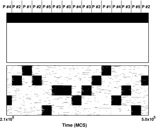
Figure 2: Sensitivity of the system under repetitive external random stimulus, as discussed in the main text. The top graph shows the Hopfield case ($\Phi=-1).$ Here, neuron activity is represented at vertical axe and simulation parameters are $N=400,$ $T=0.1$ and $\delta=0.3.$

Summing up, equations (3)–(4) provide a rather general framework to model activity–dependent processes. We here briefly reported on some consequences of adapting this to a specific case. In particular, we studied a case which describes neurobiologically–motivated fast noise, and study how this affects the synapses of an auto–associative neural network with a finite number of stored patterns. Assuming a noise distribution with a global dependence on the activity, (5), one obtains non–trivial local fields (7) which lead the system to an intriguing emergent phenomenology. We studied this case both analytically and by Monte Carlo simulations using Glauber, spin–flip dynamics [6]. We thus show that a tricritical point occurs. That is, one has (in the limit $\alpha\rightarrow 0$) first and second order phase transitions between a ferromagnetic–like, retrieval phase and a paramagnetic–like, non–retrieval phase. The noise also happens to induce a nonequilibrium condition which results in an important intensification of the network sensitivity to external stimulation. We explicitly show that the noise may turn unstable the attractor or fixed point solution of the retrieval process, and the system then seeks for another attractor. This behavior improves the network ability to detect changing stimuli from the environment. One may argue that the process of categorization in nature might follow a similar strategy. That is, different attractors may correspond to different objects, and a dynamics conveniently perturbed by fast noise may keep visiting the attractors belonging to a class which is characterized by a certain degree of correlation between its elements. A similar mechanism seems at the basis of early olfactory processing of insects [9], and instabilities of the same sort have been described in the cortical activity of monkeys [7] and other cases [8]. We are presently studying further variations of the model above.

References

- [1] Abbott L.F. and Regehr W.G.: Synaptic computation Nature 431 (2004) 796–803
- [2] Allen C. and Stevens C.F.: An evaluation of causes for unreliability of synaptic transmission Proc. Nat. Acad. Sci. 91 (1994) 10380–10383
- [3] Zador A.: Impact of synaptic unreliability on the information transmitted by spiking neurons J. Neurophysiol. 79 (1998) 1219–1229
- [4] Bibitchkov D., Herrmann J.M., and Geisel T.: Pattern storage and processing in attractor networks with short-time synaptic dynamics Network: Comput. Neural Syst. 13 (2002) 115–131
- [5] Tsodyks M., Pawelzik K., and Markram H.: Neural networks with dynamic synapses Neural Comput. 10 (1998) 821–835
- [6] Marro J. and Dickman R., Nonequilibrium Phase Transitions in Lattice Models, Cambridge Univ. Press, Cambridge 1999.
- [7] Abeles M., Bergman H., Gat I., Meilijson I., Seidelman E., Tishby N., and Vaadia E.: Cortical activity flips among quasi-stationary states Proc. Natl. Acad. Sci. USA 92 (1995) 8616–8620
- [8] Miller L.M. and Schreiner C.E.: Stimulus-based state control in the thalamocortical system J. Neurosci. 20 (2000) 7011–7016
- [9] Laurent G., Stopfer M., Friedrich R., Rabinovich M., Volkovskii A. and Abarbanel H.: Odor encoding as an active, dynamical process: experiments, computation and theory Annu. Rev. Neurosci. 24 (2001) 263–297
- [10] Cortes J.M., Torres J.J., Marro J., Garrido P.L., and Kappen H.J.: Effects of Fast Presynaptic Noise in Attractor Neural Networks Neural Comput. (2004) submitted.
- [11] Torres J.J., Garrido P.L., and Marro J.: Neural networks with fast time-variation of synapses J. Phys. A: Math. and Gen. 30 (1997) 7801–7816
- [12] Pantic L., Torres J.J., Kappen H.J., and Gielen S.C.A.M.: Associative memory with dynamic synapses Neural Comput. 14 (2002) 2903-2923