Analysis of a microscopic stochastic model of microtubule dynamic instability

Abstract

A novel theoretical model of dynamic instability of a system of linear (1D) microtubules (MTs) in a bounded domain is introduced for studying the role of a cell edge in vivo and analyzing the effect of competition for a limited amount of tubulin. The model differs from earlier models in that the evolution of MTs is based on the rates of single unit (e.g., a heterodimer per protofilament) transformations, in contrast to postulating effective rates/frequencies of larger-scale changes, extracted, e.g., from the length history plots of MTs. Spontaneous GTP hydrolysis with finite rate after polymerization is assumed, and theoretical estimates of an effective catastrophe frequency as well as other parameters characterizing MT length distributions and cap size are derived. We implement a simple cap model which does not include vectorial hydrolysis. We demonstrate that our theoretical predictions, such as steady state concentration of free tubulin, and parameters of MT length distributions, are in agreement with the numerical simulations. The present model establishes a quantitative link between microscopic parameters governing the dynamics of MTs and macroscopic characteristics of MTs in a closed system. Lastly, we use a computational Monte Carlo model to provide an explanation for non-exponential MT length distributions observed in experiments. In particular, we show that appearance of such non-exponential distributions in the experiments can occur because the true steady state has not been reached, and/or due to the presence of a cell edge.

I Introduction

Microtubules (MTs) are intracellular polymers which provide a part of the cytoskeleton and are responsible for many cell functions including division, organelle movement, and intracellular transport. A cell is a living object, and as such it has to constantly adjust to and communicate with a changing environment. For this purpose, MTs possess a property called dynamic instability, which enables them to promptly switch between two modes, growth and shortening Mitchison84 ; Hill84a ; Howard03 . This is achieved through MT having a stabilizing cap which keeps the MT from disassembling. The MT tends to depolymerize when the cap is lost Carlier81 ; Hill84a ; Hill84b ; Howard03 . The cap gradually hydrolyzes and becomes unstable as well, and so for the MT to survive it has to grow to renew its cap.

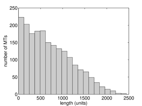
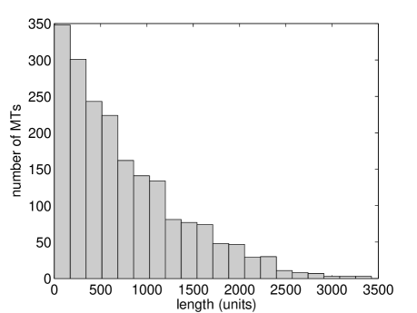
Figure 5: Histograms of MT lengths after 80 (left) and 160 (right) seconds from the beginning of polymerization. The concentration of free Tu in both cases is close to steady state value: 7.63 and 7.51 $\mu$M, respectively. Although the concentration has reached steady state after 80 sec, the length distribution of MTs is still changing. Here $K_{h}=10s^{-1}$, $c_{tot}=10\mu M$ and rest of the parameters are specified in Table 2.

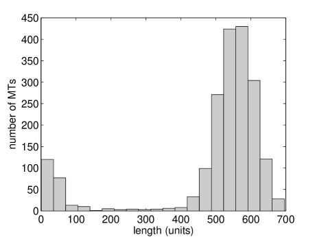
Figure 6: Histogram of MT lengths after 150 seconds from the beginning of polymerization. The concentration of free Tu is 1.382 $\mu M$ and has reached its steady state value (to within random fluctuations). $K_{h}=0.1s^{-1}$, $c_{tot}=3\mu M$ and rest of the parameters are specified in Table 2. Note the bimodal character of the distribution.

The existence of a GTP cap at the end of MTs Carlier81 and the phenomenon of dynamic instability Mitchison84 were discovered in the early 1980s. Hill and Chen used a Monte Carlo approach to simulate this behavior Hill84a ; Chen85a , employing a representation of an MT in which its cap could consist of many units (heterodimers). One of the main outcomes of their work was a suggestion that a two-phase (cap, no cap) model of dynamic instability, based only on observable macroscopic rates of phase and length changes, was sufficient to understand the behavior of the ensemble of MTs (cf. (Hill84b, , figs. 4-6)). This approach has been prevalent since then in modeling the behavior of an ensemble of MTs Dogterom93 ; Bolterauer99a ; Bolterauer99b ; Gliksman93 ; Govindan04 ; Bayley89 ; Hill84b ; Chen85b ; Freed02 ; Maly02 . One exception was the theoretical model of Flyvbjerg et al. Flyvbjerg94 ; Flyvbjerg96 which considered an elegant theoretical model of the GTP cap dynamics. This model was based on microscopic constitutuve processes of spontaneous and vectorial hydrolyses inside the MT, and fluctuating growth of the cap size. Quite recently many detailed models of a single MT began to emerge Janosi02 ; VanBuren02 ; VanBuren05 ; Stukalin04 ; Molodtsov05 which try to incorporate biological details observed recently due to advances in the experimental techniques. In particular, it is now known from the experiments that the tips of MTs can have geometrical configurations typical to growing and shortening MTs, which differ from one another (e.g., Howard03 ). This is closely related to the idea of the structural, and not necessarily a GTP cap Janosi02 , when due to tensile stresses inside the elastic body of an MT, its shape deforms from a cylinder towards the tip.

In both in vitro and in vivo experiments, dynamics of MTs have been observed under a large variety of physical conditions and in various chemical environments. Much data has been accumulated including parameter values describing the MT dynamics and length distributions. Can these values be predicted based on the conditions of the experiments? How would change in ambient conditions or the presence of spatial constraints affect observables? These questions are difficult, if not impossible, to answer using the models with postulated observable (macroscopic) rates.

In this paper we analyze a novel model of MT dynamics in a finite domain bounded by the cell edge, which involves competition of individual MTs for tubulin. The model is based on a linear 1D approximation of a MT structure. We consider the role of the boundary and extend the model to incorporate finite hydrolysis. Our model is different from earlier works Govindan04 ; Maly02 addressing the role of the edge in that we explicitly consider the concentration dependence of the dynamic instability parameters, as well as a competition for a limited tubulin pool.

Namely, we use a generalization of a microscopic model of MTs introduced in Gregoretti . Instead of postulating macroscopic rates Hill84a ; Hill84b or deducing them from numerical simulations Chen85a , we estimate them theoretically from basic microscopic rates of (de)polymerization and hydrolysis of a single unit (which can, but does not have to be interpreted as a heterodimer). This results in a higher-resolution theoretical model which may be more suitable for today’s higher-resolution experiments, and can partially address the above questions.

One of the main results of the paper is an establishment of a link, by using analytical formulas, between microscopic parameters, describing polymerization/depolymerization and hydrolysis of individual units, and macroscopic (observable) characteristics of the MT dynamics and ensemble. We demonstrate how to approximate macroscopic steady state behavior of MTs using microscopic rates and vice versa, extract microscopic rates from macroscopic behavior. Hence, it makes it possible to analytically and quantitatively predict the effect of changes in microscopic parameters on observable features, as well as to deduce microscopic changes from observed changes in macroscopic behavior, when relevant geometry and chemistry is taken into account.

We also use a computational Monte Carlo model to provide an explanation for non-exponential MT length distributions observed in experiments. In particular, we show that appearance of such non-exponential distributions in the experiments can occur because the true steady state has not been reached, and/or due to the presence of a cell edge.

The paper is organized as follows. The conceptual model and its computational implementation are presented in Section II. Next, in Section III we develop a cap model where the cap can have any number of (sub)units, which can be single heterodimers - see Figure 1B. This cap model differs from previous models in that it does not involve vectorial or induced hydrolysis. Using this model we derive approximate expressions for observable rates. We then describe in Sections IV and V a quantitative theoretical analysis of a lower-resolution model with the cap being treated as a single unit - see Figure

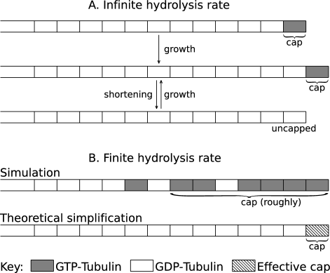
Figure 1: Schematic representation of the model.

1A. The influence of the cell edge is also studied there. Section V describes balance between polymerized and free tubulin in a bounded domain with a fixed total amount of tubulin present. Finally, we discuss and summarize our findings in Sections VI and VII.

II Model description, parameters and notations

In this section we describe a basic model of dynamics of MTs. We consider a domain of size $L_{x}\times L_{y}\times L_{z}$ with $N_{n}$ available nucleation sites for MTs in its center. $N_{n}$ is the maximal number of MTs - cf. Table

Symbol	Definition	Dimensions
$c$	concentration of free tubulin	$\mu M$
$c_{eq}^{\infty}$	critical concentration of free tubulin	$\mu M$
$c_{tot}$	total concentration of tubulin	$\mu M$
$k_{gT}$	pseudo-first order rate of adding a unit on top of a terminal T unit	$\mu M^{-1}s^{-1}$
$k_{gD}$	pseudo-first order rate of adding a unit on top of a terminal D unit	$\mu M^{-1}s^{-1}$
$\lambda$	parameter of exponential distribution (number of units)	-
$\ell$	characteristic cap size (number of units)	-
$m$	mean length (number of units) of MTs	-
$n$	coarsened step size in the cap model (number of units)	-
$\rho$	$(n-1)/(\ell-1)$	-
$K_{e}$	rate of the edge-induced catastrophe	$s^{-1}$
$K_{h}$	rate of hydrolysis (transformation to D state) of internal T units	$s^{-1}$
$K_{gT}$	rate of adding a unit on top of a terminal T unit	$s^{-1}$
$K_{gT}^{eff}$	effective rate of growing by one unit in growth phase	$s^{-1}$
$K_{gT}^{obs}$	rate of growing by $n$ units in growth phase	$s^{-1}$
$K_{gD}$	rate of adding a unit on top of a terminal D unit	$s^{-1}$
$K_{n}$	nucleation rate of a MT	$s^{-1}$
$K_{sT}$	rate of depolymerization of terminal T unit	$s^{-1}$
$K_{sT}^{eff}$	effective rate of shortening by one unit in growth phase	$s^{-1}$
$K_{sT}^{obs}$	rate of shortening by $n$ units in growth phase, = catastrophe frequency	$s^{-1}$
$K_{sD}$	rate of depolymerization of terminal D unit	$s^{-1}$
$L$	maximal length (number of units) of MTs in domain with upper bound	-
$L_{x}$, $L_{y}$, $L_{z}$	domain sizes in the numerical simulations	$m$
$M_{g}(l)$	number of MTs of length $l$ (number of units) in growth phase	-
$M_{s}(l)$	number of MTs of length $l$ (number of units) in shortening phase	-
$N_{0}$	number of free nucleation seeds	-
$N_{MT}$	number of MTs, $\leq N_{n}$	-
$N_{n}$	total number of nucleation seeds	-

Table 1: Notation highlights. The dash (-) means that the considered parameter/variable is dimensionless.

1. For simplicity, in our study of the role of the boundary (e.g., cell edge) we assume that all MTs have an identical maximal allowed length. All MTs grow from nucleation sites (there is no spontaneous nucleation), and MTs grow at one end (usually the so-called plus end) only. There is a fixed amount of total tubulin in the domain. This tubulin is present in two forms: free tubulin in the solution and polymerized tubulin constituting the MTs. Free tubulin is taken up by growing (polymerizing) MTs and is released back into the solution by shortening MTs. In general, free tubulin (Tu) diffuses inside the domain. In this paper we assume that the diffusion of free Tu is fast and does not lead to a diffusion-limited reaction rates. This is in agreement with Odde97 . Moreover, we assume uniform concentration of free tubulin throughout the domain which implies instantaneous diffusion. (For the studies of the effects of tubulin diffusion see Dogterom95 ; Deymier05 .)

In this paper a MT is represented at each moment in time in the form of a 1D straight line consisting of a certain number of units of a predefined length. Each unit belonging to a MT can be in either a growth-prone state or a shortening-prone state. We will refer to them as GTP (or T) state or GDP (or D) state respectively. All free tubulin is assumed to be in a T state. When a unit joins the MT it is initially in a T state. The probability that the internal units have hydrolyzed (transformed to a D state) increases with time. When MT disassembles (shortens) these D units, upon becoming terminal, have higher probability to disassemble and return to the solution than the terminal T units. Upon return to the solution they immediately switch to the T state. The terminal T unit does not hydrolyze but can with a certain probability depolymerize (drop from MT end). Incorporation of a new unit at the MT tip triggers the hydrolysis process of the previously terminal unit. This description seems appropriate in view of Howard03 .

The dynamics of the MTs is determined by five microscopic rates, $K_{gT}$ ($K_{gD}$) and $K_{sT}$ ($K_{sD}$), which are the rates of MT growth and shortening (i.e. adding one more unit from the solution on top of the current terminal unit, and losing this current terminal unit to the solution) when the terminal unit is in state T (D), and the hydrolysis rate $K_{h}$ of the internal units which are in state T. If the terminal unit has to hydrolyze in order to depolymerize (and its hydrolysis rate is not faster than that for the internal units) then $K_{sT}<K_{h}$.

For numerical simulations, shortening rates are taken to be independent of c while growth rates are assumed proportional to c at the location of MT tip:

$$K_{gT,gD}=k_{gT,gD}c.$$ (1)

Such specific dependence of the growth and shortening rates on c, though, is not required for many of the theoretical results we report.

When the MT reaches boundary of the domain it is not allowed to grow any more and will eventually lose its terminal unit initiating with certain probability a shortening phase. There are two more rates at the domain boundary of importance in the model: rate $K_{n}$ of nucleation from existing seeds and a rate $K_{e}$ of edge-induced catastrophe, which can also depend on c. Appendix A contains a brief description of a numerical algorithm we used in our simulations.

In what follows, we will impose restriction on a maximal length of a MT (upper bound, e.g., due to a cell edge). We will call zero a lower bound.

II.1 Observables

The standard experimental observables describing the dynamic behavior of a single MT are derived from the MT length vs. time plot. Typical length history plots of MTs are shown in Fig.

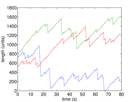
Figure 2: Length history plots of three arbitrarily selected MTs. Zero time here corresponds to 80 seconds from the start of the simulation. Here $K_{h}=10$, $c_{tot}=10$ and other parameters are listed in Table 2. See also Fig. 5.

2. Due to the two-state nature of the tubulin units inside the MT, the fluctuations in this length may be large and even in the (macroscopically) steady state each MT can repeatedly change its length all the way from zero to some characteristic length, or to the boundary. If no boundary is present and if free tubulin concentration stays high enough (if $K_{gT}$ and $K_{gD}$ are high enough) MTs can grow unbounded Dogterom93 ; Fygenson94 ; Dogterom95 . From a sawtooth-like evolution of an MT length four parameters can be extracted: the velocity/rate of growth, the velocity/rate of shortening, the average time of growth before switching to shortening, and the average time of shortening before switching to growth. The inverses of these times define the so-called catastrophe frequency and the rescue frequency, respectively. Note that brief growth or shortening intervals may pass unnoticed in the analysis of experimental data. Some models of dynamics of MTs use these four parameters as given constants for constructing analytical solutions Dogterom93 ; Govindan04 ignoring their microscopic origin. In Section III we use microscopic rates to derive the observable growth velocity and catastrophe frequency instead of setting them from the beginning.

III Cap model

Carlier and colleagues Carlier81 ; Melki90 ; Melki96 have provided experimental evidence that the GTP cap of the MTs is not restricted to the units at the very tip. This suggests that the hydrolysis is not instantaneous, a conclusion also supported by work on yeast tubulin Davis94 ; Dougherty98 . To incorporate this feature into our approach we develop a new model for the cap. In this section we show that using this model, based on the underlying microscopic laws, one can predict the observables: the catastrophe frequency and the velocity (rate) in the growth phase of MTs. In other words, the microscopic laws of the MT dynamics, governing single unit polymerization/depolymerization and hydrolysis, can be related to macro-scale (observable) dynamics of an MT.

When $K_{h}<\infty$, the MT cap in our model consists mainly of T units (cf. Fig. 1B) and possibly of a few D units and has some characteristic length (number of units) $\ell>1$. When $K_{h}\rightarrow\infty$ then $\ell=1$ because only the terminal unit is not allowed to hydrolyze and it is in a T state. Our approach is based on coarsening the resolution in the growth phase so that only blocks of the order of cap size, $n\sim\ell$, are added. By catastrophe we understand the loss of the cap. In what follows we will establish a connection between coarsened “observed” rate constants $K_{sT,gT}^{obs}$ of growing or shortening in the growth phase, and the original rates $K_{sT,gT}$ and $K_{h}$. There is no need to rescale $K_{sD,gD}$, if the free tubulin concentration is not too low. Therefore, we only consider a model for the MT cap and don’t alter the rest.

Let us consider the cap model in detail. In what follows we neglect the fluctuations in $\ell$ due to randomness in hydrolysis, and we assume that each T unit is hydrolyzed after staying an internal unit for a time $\Delta t_{h}=1/K_{h}$. After the rescue or nucleation event occurs the cap begins to grow. It has time $\Delta t_{g}+\Delta t_{h}$ to elongate, where $\Delta t_{g}=1/(K_{gT}+K_{sT})$ is the time of a single-unit step in the growth phase. After that its average length remains constant (under assumption that no catastrophe occurs during this time). For the catastrophe to occur the cap should be lost, due to fluctuations in cap size and in the growth velocity Hill84a ; Hill84b ; Odde96 . In our analysis we consider two scenarios for cap loss: (i) roughly half of the cap is lost due to random nature of MT’s growth, and the second half gets hydrolyzed during this time, or (ii) the whole cap is lost due to random fluctuations in MT growth. Keeping in mind that the terminal unit cannot be lost as a result of hydrolysis, in description (i) we require that $(\ell+1)/2$ and $(\ell-1)/2$ units are lost due to fluctuations in MT growth and propagation of hydrolysis front, respectively. We define

$$\rho=\frac{n-1}{\ell-1}.$$ (2)

In case (i) $n=(\ell+1)/2$ and $\rho=1/2$, while in case (ii) $n=\ell$ and $\rho=1$. It is important to stress that $\rho$ is introduced as a fixed parameter set a priori, based on the scenarios of cap loss similar to (i) and (ii). The two descriptions (i) and (ii) determine the duration of the coarsened step

$$\Delta t_{g}^{obs}\equiv\frac{1}{K_{gT}^{obs}+K_{sT}^{obs}}=\rho\Delta t_{h}+\Delta t_{g}\equiv\rho\cdot\frac{1}{K_{h}}+\frac{1}{K_{gT}+K_{sT}}.$$ (3)

For a given $n$, in order to rescale/coarsen the dynamics in the growth phase we require that both the average velocity and the diffusion coefficient of the MT tip remain unchanged. For a random walk on a line, with probability p to jump to the right and $q=1-p$ to jump to the left, the average velocity is $v=(p-q)\Delta x/\Delta t$ and the diffusion coefficient is $D=2pq\Delta x^{2}/\Delta t$. Here $\Delta x$ is the step length and $\Delta t$ is the time per step. In case of the original walk $p=p_{g}=K_{gT}\Delta t_{g}$, $\Delta x=1$ and $\Delta t=\Delta t_{g}$, while in case of the rescaled walk $p=K_{gT}^{obs}\Delta t_{g}^{obs}$, $\Delta x=n$ and $\Delta t=\Delta t_{g}^{obs}$ is given by eq. (3). After introducing the effective rates of adding or losing one unit (as opposed to one block),

$$K_{gT,sT}^{eff}\equiv nK_{gT,sT}^{obs},$$ (4)

and using conservation of $v$ and $D$ we obtain that

$$K_{gT}^{eff}-K_{sT}^{eff}=K_{gT}-K_{sT}$$ (5)

$$\frac{K_{gT}^{eff}K_{sT}^{eff}n}{K_{gT}^{eff}+K_{sT}^{eff}}=\frac{K_{gT}K_{sT}}{K_{gT}+K_{sT}}.$$ (6)

From eqs. (3) and (4) $n/(K_{gT}^{eff}+K_{sT}^{eff})$ can be found and substituted into eq. (6), resulting in

$$K_{gT}^{eff}K_{sT}^{eff}=\beta,$$ (7)

where

$$\beta\equiv\frac{K_{gT}K_{sT}}{1+\rho\cdot{\displaystyle\frac{K_{gT}+K_{sT}}{K_{h}}}}.$$ (8)

After solving Eqs. (5) and (7) and choosing only positive solutions we obtain that

$$K_{gT}^{eff}=\frac{K_{gT}-K_{sT}+\sqrt{(K_{gT}-K_{sT})^{2}+4\beta}}{2}$$ (9)

$$K_{sT}^{eff}=\frac{-K_{gT}+K_{sT}+\sqrt{(K_{gT}-K_{sT})^{2}+4\beta}}{2}.$$ (10)

Expression (9) displays some expected features. Namely, when $K_{h}\rightarrow\infty\Rightarrow K_{gT}^{eff}\rightarrow K_{gT}$ and when $K_{h}\rightarrow 0\Rightarrow K_{gT}^{eff}\rightarrow(K_{gT}-K_{sT}+|K_{gT}-K_{sT}|)/2=\left[\begin{array}[]{cc}K_{gT}-K_{sT},&K_{gT}\geq K_{sT}\\ 0,&K_{gT}\leq K_{sT}\end{array}\right.$. In general, $\max(0,K_{gT}-K_{sT})\leq K_{gT}^{eff}\leq K_{gT}$.

Eq. (6) combined with eqs. (9) and (10) yields

$$n=\frac{K_{gT}K_{sT}}{K_{gT}+K_{sT}}\frac{\sqrt{(K_{gT}-K_{sT})^{2}+4\beta}}{\beta}$$ (11)

and eq. (2) can now be used to determine $\ell$. On the other hand, $\ell$ can be approximated as follows:

$$\ell\approx K_{gT}^{eff}\Delta t_{h}+1=\frac{K_{gT}^{eff}}{K_{h}}+1,$$ (12)

where the term $K_{gT}^{eff}\Delta t_{h}$ approximates the number of added units after the beginning of a growth phase, before the hydrolysis front starts moving. In fact, eq. (12) can be used as a definition of $\ell$ and n can be found from eq. (2). Then there is no need for eq. (3) as eqs. (5), (6) and (12) form a closed set of equations. This approach, however, leads to a cubic equation for $K_{gT}^{eff}$, while in the above approach we need to solve a quadratic equation, which is much simpler. Nevertheless, the definition of $\ell$ through eq. (12) seems to work better in the limit of $K_{gT}\rightarrow 0$. Namely, substituting eq. (12) into eq. (2) yields $n=1+\rho K_{gT}^{eff}/K_{h}$ and the only non-negative solution of this equation together with eqs. (5) and (6), in the limit $K_{gT}\rightarrow 0$, is $K_{gT}^{eff}=0$, $K_{sT}^{eff}=K_{sT}$ and $n=1$. Indeed, it seems reasonable to postulate that $n\rightarrow 1$, i.e., there is no rescaling, when $K_{gT}\rightarrow 0$. This does not follow from eqs. (8) and (11), which lead to $n\rightarrow 1+\rho K_{sT}/K_{h}>1$ instead.

Using the above developments, it is possible to derive scaling behaviors of various quantities as functions of, e.g., c and $K_{h}$. For example, substituting eqs. (2) and (12) into eq. (8) and using eq. (7) together with eq. (4) leads to

$$\begin{array}[]{ccc}K_{sT}^{obs}&\approx&{\displaystyle\frac{1}{n}\cdot\frac{K_{gT}K_{sT}}{K_{gT}^{eff}+(n-1)(K_{gT}+K_{sT})}}\\ \\ &\approx&\left[\begin{array}[]{cc}{\displaystyle\frac{K_{sT}}{n^{2}}},&K_{gT}\gg K_{sT}\\ \\ {\displaystyle\frac{K_{sT}}{2n(n-1)}},&K_{gT}\gg K_{gT}^{eff}\end{array}\right.,\end{array}$$ (13)

so that the catastrophe rate (frequency) $K_{sT}^{obs}$ scales as $n^{-2}\propto\ell^{-2}$. This is characteristic of diffusive scaling because time to catastrophe is determined by diffusive movement of the hydrolysis front relative to the MT tip. If free tubulin concentration c is not too small, then eqs. (11), (8) and (1) yield $n\propto c$ and hence $K_{sT}^{obs}\propto c^{-2}$, which is in at least qualitative agreement with previous predictions Chen85b ; Mitchison87 . The scaling $K_{sT}^{obs}\propto n^{-2}$ might have been postulated, as well, which would have led us to an additional version of the solution of the cap model.

To provide another scaling example, let us now assume that $K_{h}$ is small and $K_{gT}\approx K_{sT}$. Then from eq. (8) it follows that $\beta\approx K_{h}K_{sT}/(2\rho)\propto K_{h}$. If $\beta\gg(K_{gT}-K_{sT})^{2}$, i.e., if $K_{h}$ is not too small, then eq. (11) yields $n\propto K_{h}^{-1/2}$ and hence $\ell\propto K_{h}^{-1/2}$ as well. Notice, that it is the same scaling as derived for actin polymers (Vavylonis05, , eq.3).

IV Ensemble dynamics of microtubules

In this section we treat cap as a single effective unit - cf. Fig. 1. Thus the model essentially reduces to the two-phase model proposed in Hill84b . First, we rederive length distribution of MTs, which are known in the literature. In particular, we study the role of upper bound (e.g., cell edge). We use these results for analyzing in the next section competition for a finite tubulin pool. We also consider the steady state critical concentration of free Tu.

In what follows, we use either the discrete or the continuous description of MT dynamics, whichever is convenient. We assume that the continuous model provides a good approximation of the discrete model. The continuous approach was discussed in Hill87 ; Verde92 ; Dogterom93 while an analogous discrete approach was developed in Hill84b ; Govindan04 . Following Dogterom93 we write down the equations for length distributions of MTs in growth and shortening phases in the form

$$\partial_{t}M_{g}=-K_{sT}^{obs}M_{g}+K_{gD}M_{s}-K_{gT}^{eff}\partial_{l}M_{g}$$ (14)

$$\partial_{t}M_{s}=K_{sT}^{obs}M_{g}-K_{gD}M_{s}+K_{sD}\partial_{l}M_{s},$$ (15)

where $M_{g,s}(l,t)$ are densities of MTs of length $l$ at time $t$, in the growing (g) and shortening (s) phases.

Equations (14) and (15) can be used to describe regular diffusion with drift, if we don’t distinguish between the phases (see also Maly02 ). However, it is important to stress that these equations don’t have diffusion terms for $M_{g,s}(l,t)$ and hence switching phases back and forth is the only mechanism of spreading of these distributions present. This is in agreement with our simulations in the case of instantaneous hydrolysis of internal units. Notice that diffusion terms are used in Hill84b .

First, consider a semi-infinite domain. Equations (14) and (15) with the boundary condition $M_{g,s}(l=\infty)=0$ have the following steady state solution

$$M_{g}=Ae^{-l/\lambda},$$ (16)

$$M_{s}=\frac{K_{gT}^{eff}}{K_{sD}}Ae^{-l/\lambda},$$ (17)

where

$$\frac{1}{\lambda}\equiv\frac{K_{sT}^{obs}}{K_{gT}^{eff}}-\frac{K_{gD}}{K_{sD}}.$$ (18)

The necessary condition for the existence of a steady state in the case without a boundary is given by $\lambda>0$. The prefactor $A$ is a normalization coefficient which depends on the total number of MT nucleation seeds present and on the nucleation probability.

We now add a constraint limiting the maximal length of MTs to be $L$. MTs cannot become longer due to a barrier, for example a cell edge, as is often the case in vivo, especially when the cell is in the interphase and the MTs are relatively long. For simplicity we assume that $L$ is identical for all MTs. We still can use eqs. (14) and (15) inside the domain, for $0<l<L$, and consider a steady state. Adding up these two equations then leads to $\partial_{l}(-K_{gT}^{eff}M_{g}+K_{sD}M_{s})=0,$ which means that the spatial derivative of the flux (of the MT tips, considered as random walkers) is zero meaning that the flux is uniform. However, in the closed system this flux must be zero and hence

$$M_{s}=\frac{K_{gT}^{eff}}{K_{sD}}M_{g}.$$ (19)

It follows that eqs. (16), (17) and (18) still hold inside the domain, except for $\lambda$ not being necessarily positive, which is in agreement with previous work Govindan04 . This means qualitatively that there might be a steady state distribution of MTs in which most of them are close to the upper boundary (e.g., cell edge), while only a few are short.

IV.1 Critical concentration of free tubulin

Let us consider the limiting case $1/\lambda=0$ (cf. eq. (18)). This defines the upper limit of the concentration of free tubulin $c_{eq}^{\infty}$ at which the steady state in the semi-infinite domain still exists (cf. Dogterom93 ). Let us use eq. (1) and define

$$\begin{array}[]{ccc}a={\displaystyle\frac{K_{sT}}{k_{gT}}},&&b={\displaystyle\sqrt{\frac{K_{sT}K_{sD}}{k_{gT}k_{gD}}}}.\end{array}$$ (20)

Because the MTs in the growth phase are less likely to shorten than are MTs in the shortening phase, $a<b$. In general, $c_{eq}^{\infty}\in[a,b]$. Notice that slowdown of hydrolysis reduces $c_{eq}^{\infty}(K_{h})$. When hydrolysis is instantaneous then c reaches its maximal value $c_{eq}^{\infty}(\infty)=b$. When there is no hydrolysis at all then $c_{eq}^{\infty}(K_{h})$ reaches its minimal value $c_{eq}^{\infty}(0)=a$ meaning that the average growth rate in this case, $k_{gT}c_{eq}^{\infty}(0)-K_{sT}$, is zero.

One can get a scaling estimate of $c_{eq}^{\infty}$ if it is far enough from both $a$ and $b$. Assume that $K_{gT}\gg K_{sT}$ and $K_{gT}\gg K_{h}$. Using eq. (1), then $K_{gT}^{eff}\approx K_{gT}\propto c$. Now, $\rho$ is of order of 1, so that from eq. (8) and eq. (11) it follows that $\beta\sim K_{sT}K_{h}\ll K_{gT}^{2}$ and $n\sim K_{gT}/K_{h}\propto c/K_{h}$, respectively. Hence $K_{sT}^{obs}\approx K_{sT}/n^{2}\propto(K_{h}/c)^{2}$. Substituting these scaling relations into $1/\lambda=0$ and using eq. (18) yields $c_{eq}^{\infty}\propto\sqrt{K_{h}}$.

Notice that if there are no rescues, $k_{gD}=0$, then $c_{eq}^{\infty}$ is infinite (see also Mitchison87 ) and unbounded growth can not happen. This is so because without rescues the MT depolymerizes completely after the catastrophe, no matter how long it was before.

V Competition for tubulin

In Section IV we have shown the existence of a steady state distribution of MTs inside a domain. It is conceivable that by sensing and controlling free tubulin concentration and the number of MTs the cell regulates MT dynamics, as suggested in Mitchison87 ; Gregoretti . In what follows we show in detail how to determine a steady state concentration of free tubulin c, which is the key to finding steady state characteristics of MTs in a closed system. The main goal of this section is to derive expressions for the average number of units per MT $m$, and a number of MTs $N_{MT}$ as functions of $c$ and the other parameters. These functions are needed to determine c from the conservation of total tubulin. Because m can not extend beyond the domains’ boundary, and because $N_{MT}$ is less or equal than a number of nucleation sites $N_{n}$, the number of polymerized units in a bounded domain stays restricted as the amount of total Tu grows.

In what follows we assume that the total amount of tubulin is constant and we consider bounded domain of volume $V$. We also assume instantaneous diffusion so that the concentration of free tubulin is uniform throughout the domain. Hence,

$$N_{tot}=N_{free}+mN_{MT},$$ (21)

where $N_{tot}$ is a total number of tubulin units in the domain and $N_{free}$ is a number of free tubulin units. By dividing this formula by $V$ we obtain expression for concentrations measured in micromolars ($\mu M$)

$$c_{tot}=c+\frac{mN_{MT}}{10^{-3}N_{A}V},$$ (22)

where $V$ is given in $m^{3}$ and $1\mu M$ is equal to $10^{-6}N_{A}$ units per liter or $10^{-3}N_{A}$ units per $m^{3}$; $N_{A}\approx 6.022\times 10^{23}\textrm{mol}^{-1}$ is the Avogadro’s constant. We will use this expression for studying MTs in cases of unbounded and bounded domains.

V.1 Unbounded domain

It has been shown in Section IV that the steady state distribution of MT lengths in this case is exponential as described by eqs. (16) and (17) with $\lambda$ representing mean length of a MT

$$m=\lambda.$$ (23)

To find $N_{MT}$ for a given $N_{n}$, we use a balance equation for the number of available nucleation sites $N_{0}\equiv N_{n}-N_{MT}$:

$$K_{sT}^{obs}M_{g}(l=1)+K_{sD}M_{s}(l=1)=K_{n}N_{0},$$ (24)

where $K_{n}$ is a nucleation rate, which in general depends on $c$. The left-hand side of eq. (24) describes the rate of production of available nucleation sites by completely depolymerizing MTs. The first term represents those MTs which experience a catastrophe, while the second term stands for those MTs which are already in the shortening phase. Using (16), (17), and assuming that $\lambda\gg 1$, yields

$$A(K_{sT}^{obs}+K_{gT}^{eff})\approx K_{n}N_{0}.$$ (25)

In addition, approximating summation by integration as follows

$$N_{MT}=\sum_{l=1}^{\infty}\left(M_{g}(l)+M_{s}(l)\right)\approx\left(1+\frac{K_{gT}^{eff}}{K_{sD}}\right)A\lambda$$ (26)

results in

$$N_{MT}\approx\frac{N_{n}}{1+{\displaystyle\frac{K_{sT}^{obs}+K_{gT}^{eff}}{\lambda K_{n}(1+K_{gT}^{eff}/K_{sD})}}}.$$ (27)

Substituting eqs. (23), (27) and (18) into eq. (22), and using dependence of the rates on concentration c, eq. (1), yields an equation $c_{tot}=F(c)$, at steady state. This equation relates free tubulin concentration c and total concentration $c_{tot}$, as a function of all given parameters.

V.2 Bounded domain

Here again we impose limitation on the maximal possible length of MTs not to exceed L. In the case of a bounded domain a steady state solution of eqs. (14) and (15) can be calculated, and then $m$ and $N_{MT}$ are determined in a way similar to the previous case. Notice that the steady state does exist even if $c>c_{eq}^{\infty}$. Since $0\leq m\leq L$ and $0\leq N_{MT}\leq N_{n}$ always hold, the second term in eq. (22) is non-negative and bounded. Therefore, when c goes from 0 to $\infty$ so does $c_{tot}$. If the right-hand side of eq. (22) monotonically increases with c then there is a unique physically meaningful c for each $c_{tot}$, at steady state.

It is shown in Appendix B that now

$$N_{MT}\approx\frac{N_{n}}{1+{\displaystyle\frac{K_{sT}^{obs}+K_{gT}^{eff}}{K_{n}\left[(1+K_{gT}^{eff}/K_{sD})(1-e^{-L/\lambda})\lambda+(K_{gT}^{eff}/K_{e})(1+K_{gD}/K_{sD})e^{-L/\lambda}\right]}}}$$ (28)

and

$$m\approx\frac{(1+K_{gT}^{eff}/K_{sD})\lambda(\lambda-e^{-L/\lambda}(L+\lambda))+L(K_{gT}^{eff}/K_{e})(1+K_{gD}/K_{sD})e^{-L/\lambda}}{(1+K_{gT}^{eff}/K_{sD})\lambda(1-e^{-L/\lambda})+(K_{gT}^{eff}/K_{e})(1+K_{gD}/K_{sD})e^{-L/\lambda}}.$$ (29)

When $\lambda>0$ and $L\rightarrow\infty$ eqs. (28) and (29) reduce to eqs. (27) and (23), respectively. When $K_{gT}^{eff}\rightarrow 0$ and $K_{gD}\rightarrow 0$, then $\lambda\downarrow 0$ (so that $\lambda>0$), $N_{MT}\rightarrow 0$ and $m\rightarrow 0$. When $K_{gT}^{eff}\rightarrow\infty$ and $K_{gD}\rightarrow\infty$, then $\lambda\uparrow 0$ (so that $\lambda<0$), $N_{MT}\rightarrow N_{n}$ and $m\rightarrow L$, as expected.

VI Discussion of the results

VI.1 Comparison with existing cap models

The cap model presented in this paper differs from the approaches used in Hill84a ; Hill84b ; Flyvbjerg94 ; Flyvbjerg96 . First, we don’t postulate catastrophe frequency and growth velocity, or derive them from numerical simulations, as was done in Hill84a ; Hill84b . Instead, we analytically derive these macroscopic rates from small-scale rates (such as chemical rate constants). Second, we employ only spontaneous hydrolysis and don’t use induced, or vectorial, hydrolysis; both types of hydrolysis were used in Flyvbjerg94 ; Flyvbjerg96 . Our model agrees with the experimental data analyzed in Flyvbjerg94 ; Flyvbjerg96 as can be seen from the main panel in Fig.

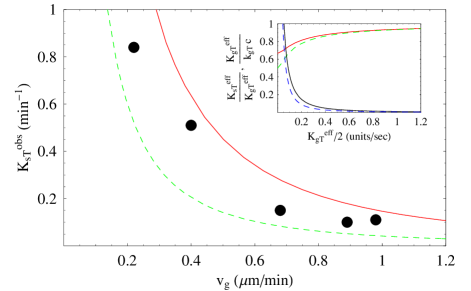
Figure 3: Frequency of catastrophe $K_{sT}^{obs}$ as a function of MT growth velocity $v_{g}$. Dots represent experimental data Drechsel92 ; Flyvbjerg94 . Solid and dashed lines correspond to $\rho=1/2$ and $\rho=1$, respectively, and were obtained using the model (Section III). Inset: Two upper curves on the right are $K_{gT}^{eff}/K_{gT}$ and two lower curves on the right are $K_{sT}^{eff}/K_{gT}^{eff}$.

3. Specifically, the predicted dependence of the catastrophe frequency on MT growth velocity is in agreement with experimental data.

The cap dynamics in the model proposed by Flyvbjerg et al. Flyvbjerg94 ; Flyvbjerg96 is modeled by addition of tubulin from the solution to the MT tip. This addition (polymerization) is faster than the propagation of the induced hydrolysis front (low end of the cap). Therefore, the cap length would grow infinite were it not for the spontaneous hydrolysis at some point inside the cap. When it occurs, the cap is redefined as an interval between this spontaneous hydrolysis point and the MT tip. In this way, the average cap size can be kept constant at steady state. According to Flyvbjerg et al. Flyvbjerg94 ; Flyvbjerg96 , catastrophe occurs when this cap is lost, and it is postulated that the remaining GTP-Tu units below the cap are not capable of rescuing the MT. This assumption is made in order to allow for catastrophe to occur. Otherwise, in many cases the rescue would immediately follow the cap loss. While this picture is widely accepted, in our alternative model the picture is even simpler. We use only one type of hydrolysis and we don’t need to make any additional assumptions. In our model, there is a hydrolysis front due to spontaneous hydrolysis of old enough units (see Section III). The velocity of this front is governed by the age of the units inside the MT and hence it is always approximately equal (with fluctuations) to the growth velocity. Faster growth velocity leads to a longer cap, reducing the catastrophe frequency.

Dilution experiments have shown that sharp reduction in the concentration of free Tu to low or zero values results in collapse of the MTs after a certain delay. Importantly, this delay is practically independent of the initial free Tu concentration Walker91 . Flyvbjerg et al. explain this phenomenon by arguing that the dilution results in domination of spontaneous hydrolysis which regulates the waiting time before the collapse. Therefore, this time is almost independent of the initial cap size. Our model yields the following simple explanation. When concentration of free Tu becomes very low, two events must occur for the cap to disappear. The terminal unit should be lost (rate $K_{sT}$) and the next unit should hydrolyze (rate $K_{h}$). If this next to last unit is old enough to hydrolyze then, with high probability, the rest of the cap has already hydrolyzed.

Dilution experiments reported in Walker91 and cited in Flyvbjerg94 determine the average waiting time before the catastrophe as roughly 5-10s. Therefore, in Fig. 3 we set $K_{h}=K_{sT}=0.15s^{-1}$. If the shortening velocity ($K_{sD}$) is much larger than $K_{sT}$, and if the loss of the terminal unit is conceptualized as a two-stage process of hydrolysis and then falling, the equality $K_{h}=K_{sT}$ would indicate that the hydrolysis rate of the terminal unit equals the hydrolysis rate of the internal unit. Notice that we were not able to fit the catastrophe frequency data if $K_{sT}$ and $K_{h}$ were significantly different. In the dilution experiments spatial resolution was about $0.25\mu m$ Walker91 , which is about 30 heterodimers (per protofilament), so that actual waiting time before losing the terminal unit (heterodimer) might be faster than the reported waiting time before the collapse. We used eq. (1) with $k_{gT}=0.3\mu M^{-1}s^{-1}$, however any value of $k_{gT}$ can be used, because it enters the formulas only through $K_{gT}=k_{gT}c$ and there is no explicit c-dependence in the figure. The unit length is taken to be the length of one heterodimer of Tu, 8nm and hence $1\,unit/s\approx 0.5\,\mu m/min$. Therefore $v_{g}\,(\mu m/min)\approx K_{gT}^{eff}/2\,(units/s)$. In the inset of Fig. 3 we show the values of $K_{sT}^{eff}/K_{gT}^{eff}$ and $K_{gT}^{eff}/K_{gT}$. It is seen that for $v_{g}>0.2$ one has $K_{sT}^{obs}<K_{sT}^{eff}\ll K_{gT}^{eff}$ and hence $v_{g}\propto K_{gT}^{eff}\propto c$.

VI.2 Competition for tubulin and the edge effect

Here we study competition for a limited pool of free tubulin and combine it together with the cap model. At steady state, the dependence of free tubulin concentration, c, on the total tubulin concentration, $c_{tot}$, is governed by tubulin mass conservation eq. (22). The resulting value of c, in turn, defines the dynamics of MTs and their ensemble distributions.

In the case of an unbounded spatial domain, we have reproduced the prediction of the Oosawa and Kasai model Oosawa62 including existence of a critical concentration of free tubulin $c_{eq}^{\infty}$ (see thin lines in Fig.

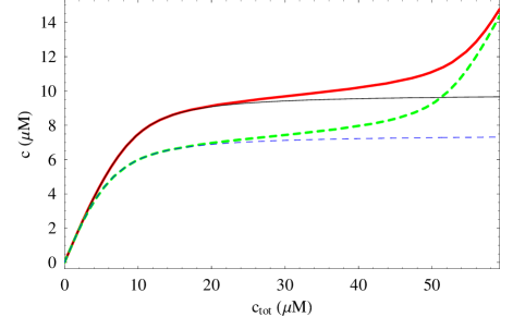
Figure 4: Steady state concentration of free vs. total Tu in the unbounded (thin lines) and bounded (thick lines) domains. For a bounded domain maximal MT length L is roughly 1400 units. For a bounded domain c reaches its asymptotic value $c_{eq}^{\infty}(K_{h})$. Hydrolysis rate is $K_{h}=10s^{-1}$. Full and dashed lines correspond to $\rho=1/2$ and $\rho=1$, respectively. Other parameters are $N_{n}=200$, $V=10^{-17}m^{3}=10^{-8}\mu\textrm{L}$, $k_{gT}=5\mu M^{-1}s^{-1}$, $K_{sT}=5s^{-1}$, $k_{gD}=0.5\mu M^{-1}s^{-1}$, $K_{sD}=500s^{-1}$, $K_{n}=K_{gD}$, $K_{e}=K_{sT}$, and we use eq. (1).

4). The steady state cannot exist above this value. Depending on the choice of parameters, the transition from almost linear growth of c, $c\approx c_{tot}$ for low $c_{tot}$, to the asymptotic value $c=c_{eq}^{\infty}$ can be made sharp or smooth. (In Oosawa model, this transition is assumed to be sharp meaning that when $c_{tot}<c_{eq}^{\infty}$ there are no MTs and when $c_{tot}>c_{eq}^{\infty}$ all the excess tubulin above $c_{eq}^{\infty}$ goes into polymerized state.) When the probability of rescue is zero then $c_{eq}^{\infty}\rightarrow\infty$, our model describes the situation considered in Mitchison87 .

If there is an upper bound on MT lengths, then at sufficiently high concentrations of total tubulin, this bound inhibits further polymerization of MTs (edge effect). Hence, the steady state free tubulin concentration can rise above its critical value. This edge effect is demonstrated by thick lines in Fig. 4 and was first discussed in Gregoretti . Under our reference conditions, it is seen that for $c_{tot}>20\mu M$ the edge starts playing an important role. At sufficiently high $c_{tot}$, the edge reestablishes linear growth of c with respect to $c_{tot}$. The implications of this effect are as follows. If $c_{tot}$ is high enough, the MTs grow persistently up until hitting the edge which triggers their catastrophe. This is consistent with recent experimental observations of persistent growth of MTs in vivo Komarova02 . From our model it follows that by changing the number of nucleation sites while keeping the total amount of Tu constant the cell could regulate the transition between mitotic (short) and interphase (long) MTs.

Next we compare in Table

Parameters			Simulated results				Theoretical estimates: $n=(\ell+1)/2$, $n=\ell$ (see text)
$K_{h}$	$c_{tot}$	$N_{n}$	$c$	$m$	$\frac{\#T}{N_{n}}$	$N_{MT}$	$c_{eq}^{\infty}$	$c$	$\lambda$	$\ell$	$\frac{K_{gT}^{eff}}{K_{h}}+1$	$N_{MT}$
$\infty$	36	2000	31.32	1416	0.759	1990	31.62	31.28	1430	1	1	1989
$\infty$	28	3000	27.46	117	0.734	2814	-”-	27.48	112	1	1	2797
$\infty$	28	$10^{4}$, T seed	26.48	92.7	0.780	9908	-”-	26.53	89.5	1	1	9909
$10^{5}$	36	2000	31.36	1401	0.997	1995	31.60, 31.57	31.25, 31.23	1437, 1444	1.0015	1.0016	1989
100	30	2000	20.78	2788	1.75	1992	21.05, 17.38	20.92, 17.29	2742, 3836	2.00, 1.82	2.03, 1.84	1994, 1996
30	15	2000	12.7	694	2.69	1969	14.7, 11.5	13.9, 11.2	347, 1139	3.16, 2.72	3.22, 2.77	1952, 1985
10	10	2000	7.51	758	3.94	1974	9.85, 7.48	9.02, 7.18	305, 857	5.04, 4.12	5.16, 4.20	1945, 1980
10	5	2000	4.91	35.1	2.25	1538	-”-	4.95, 4.85	21.9, 52.1	3.06, 2.98	3.20, 3.07	1420, 1722
3	5	2000	3.94	327	5.66	1954	6.08, 4.59	4.64, 3.99	115, 312	7.22, 6.09	7.42, 6.21	1868, 1952
1	4	2000	2.56	443	8.51	1958	3.90, 2.99	3.24, 2.63	237, 420	12.5, 9.42	12.77, 9.53	1941, 1970
0.3	5	2000	1.795	971	14.0	1988	2.50, 2.00	2.31, 1.86	817, 950	23.6, 16.1	23.7, 16.1	1986, 1990
0.1	3	2000	1.379	496	19.8	1970	1.782, 1.510	1.573, 1.368	433, 494	32.1, 21.5	31.6, 20.8	1982, 1988
0.03	3	2000	1.192	553	32.9	1969	1.368, 1.234	1.262, 1.163	526, 555	50.7, 33.2	48.5, 31.1	1991, 1994
0.01	2	2000	1.080	286	42.5	1937	1.179, 1.112	1.097, 1.058	273, 284	65.6, 43.2	58.4, 37.0	1992, 1995

Table 2: Comparison of simulated and theoretical results. All values reported here are at or very close to steady state. Cells containing two numbers show theoretical predictions for $\rho=1/2$ and 1, respectively. Domain size is $L_{x}=L_{y}=10^{-4}$ and $L_{z}=10^{-7}$ (m). It is ensured that the domain is long enough so that the MTs don’t reach the boundary for the given parameters. Here $k_{gT}=5$, $K_{sT}=5$, $k_{gD}=0.5$, $K_{sD}=500$, $K_{gT,gD}=k_{gT,gD}c$. For nucleation rate we use $K_{n}=K_{gD}$, i.e., a D seed, except for the third line, where it is a T seed, $K_{n}=K_{gT}$. $\#T/N_{n}$ is an estimate for the cap size - see Section VI.2. Initially all Tu is free and its concentration is $c_{tot}$. Notice that $c<c_{eq}^{\infty}$.

2 Monte Carlo simulations (see Appendix A) with the results obtained by using our continuous model. We choose large domain size so that MTs never reach the boundary and $m=\lambda$ (cf. Eq. (23)). We run simulations for different parameter sets until steady state is reached and then determine free tubulin concentration, number of MTs and their mean length, and estimate the cap size. Recall that only MTs in growth phase have caps. Therefore, we estimate the cap size $\ell$ of MTs in our simulations by $\ell\sim(1+K_{gT}^{eff}/K_{sD})\cdot\#T/N_{MT}$, where $\#T$ is the number of polymerized Tu units in T state. We also use eq. (19). For the parameter values used in Table 2 simplified formula for the estimated cap size $\ell\sim\#T/N_{n}$ has been used.

Table 2 also contains theoretical estimates corresponding to the simulated values discussed above. In addition, the table includes theoretical estimates of $c_{eq}^{\infty}$ and of the cap size based on eq. (12). In most cases the simulated results lie in between our two theoretical approximations, for $\rho=1/2$ and $\rho=1$ respectively, in agreement with the model description of cap evolution. These approximations are given as two adjacent numbers in the cells of the table displaying our theoretical estimates. When, however, $K_{h}$ becomes small, and c approaches a (eq. (20)), our approximations seem to consistently overestimate the number of MTs, $N_{MT}$. This should be improved by rescaling the rest of the rates, $K_{gD}$, $K_{sD}$, $K_{n}$ and $K_{e}$, which is outside of the scope of this paper.

VI.3 Non-steady-state phenomena

Our numerical simulations are also capable of reproducing and explaining two other phenomena observed in experiments. Specifically, (i) in some cases the non-exponential MT length distribution and (ii) decaying oscillations in free tubulin concentration have been observed.

MT length distributions. It is often mentioned in the literature that the steady state length distribution of MTs observed in the experiments is either exponential or bell-shaped Gliksman93 ; Gliksman92 ; Cassimeris86 ; Verde90 ; Bolterauer99a ; Bolterauer99b . Exponential distribution agrees with our model. Inability to obtain a bell-shaped distribution seems to indicate a limitation to our model. While we don’t exclude the possibility that some rates might depend on the MT length, as proposed by Bolterauer99a ; Bolterauer99b , or on time spent in a given phase Odde95 ; Odde98 , we suggest two alternative ways of obtaining bell-shaped distributions under certain conditions. First, one should be careful in determining when the system reaches the steady state in the experiment or simulation. As our simulations demonstrate, the system reaches the constant free tubulin concentration and MTs reach constant mean length relatively quickly. (The number of MTs does not change much henceforth.) By that time the MT length histogram is often bell-shaped as illustrated in Fig.

5 and Fig.

6. This can be explained as follows. When MTs start growing from nucleation sites there is an excess of free tubulin. Therefore, the growth is originally unbounded leading to a Gaussian shape. If the cell edge (upper boundary) is far away, in the course of this growth the free tubulin concentration drops and reaches its steady state value. At this time the shape can still be close to a Gaussian (cf. (Gliksman93, , fig. 4)). This is followed by a long process of a shape change of the MT length histogram with free tubulin being constant. Eventually, this results in an exponential shape and in system reaching true steady state. This situation is well described in OShaughnessy03a ; OShaughnessy03b .

A bell-shaped distribution can be also obtained in a bounded domain when the steady state concentration of free tubulin is high enough for unbounded growth of MTs if it were not for a cell edge (i.e., if $c>c_{eq}^{\infty}$). In this situation we predict positive exponential distribution of MT lengths, in the case when all MTs can reach identical maximal length restricted by the edge, consistent with Govindan04 ; Maly02 . As can be seen in experiments, however, MTs are curved and cell shape is not ideally spherical or circular, so that different MTs experience different restrictions (e.g., Cassimeris86 ; Komarova02 ). This can lead to an MT length histogram of a bell-shaped form, in true steady state.

Oscillations. In some of the simulations we observed an overshoot in free Tu concentration before the steady state was reached. Moreover, in some cases there were slight oscillations of free Tu concentration, as shown in Fig.

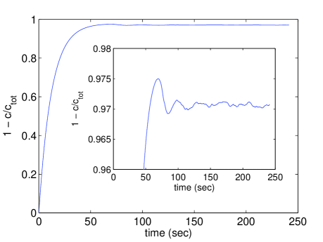
Figure 7: Small oscillations in the amount of polymerized Tu observed in numerical simulations for $K_{h}=0.1s^{-1}$, $c_{tot}=50\mu M$ and $N_{n}=10^{4}$. Other parameters are as in Table 2. Inset is a blowup of the region of oscillations.

7. Overshoots and large oscillations have been reported and modeled in the literature Carlier87 ; Chen87 ; Bayley89 ; Jobs97 ; Bolterauer99b ; Sept99 ; Sept00 ; Deymier05 . It is believed that slow conversion of D- into T-tubulin in solution, after the depolymerization, is the key to understanding of such oscillations. These oscillations occur if initial free Tu concentration is sufficiently large.

Free D-tubulin cannot polymerize. In our model we assume its conversion into T-tubulin to be instantaneous. We also use linear (and not higher order) dependence of nucleation rate on free Tu concentration, and a fixed number of nucleation sites. It is remarkable that under these restrictive assumptions the model produced some oscillations. We suggest the following explanation for their existence. If the hydrolysis is slow enough, the MTs grow quickly in the beginning, resulting in a large cap. When free Tu concentration changes quickly, the cap needs a relatively long time to adjust. This leads to a delayed response, and possibly to oscillations. Hence it might be that the ability to produce oscillations is inherent to MT structure, and that it can be magnified under certain experimental conditions.

VII Conclusions

In this paper we analyze a novel model of MT dynamics in a domain bounded by the cell edge which involved competition of individual MTs for tubulin. The model is based on a linear 1D approximation of a MT structure. We consider the role of the boundary and extended the model to incorporate finite hydrolysis.

One of the main results of the paper is an establishment of a link, by using analytical formulas, between microscopic parameters describing polymerization/depolymerization and hydrolysis of individual units, and macroscopic (observable) characteristics of the MT dynamics and ensemble. We demonstrate how to approximate macroscopic steady state behavior of MTs using microscopic rates and vice versa, extract microscopic rates from macroscopic behavior. Hence, it is possible to analytically and quantitatively predict the effect of changes in microscopic parameters on observable features, as well as to deduce microscopic changes from observed changes in macroscopic behavior, when relevant geometry and chemistry is taken into account.

We consider the cell edge, and derive expressions characterizing MT distributions in the case of a finite pool of tubulin units. We perform Monte Carlo simulations to compare with our theoretical results, and find a good agreement between the two.

The key ingredient in establishing a link between micro- and macro-parameters is the cap model, which allows one to replace the actual cap consisting of many units by an effective single unit. The cap model behavior agrees with experiments measuring catastrophe frequency as a function of free tubulin concentration as well as with dilution experiments.

We also use computational Monte Carlo model to provide an explanation for a non-exponential MT length distributions observed in experiments.

We plan to develop in future a detailed model for an individual MT which will take into account the MT protofilament structure, and to use this model for investigating effects of various MAPs on the dynamic instability.

Appendix A Computational model

In what follows we provide a short description of the numerical algorithm used for our simulations, which slightly differs from that used in Gregoretti . At time zero, MTs begin to grow from the nucleation seeds. At each simulation step, the time of this step is calculated by defining the rates of change in length (either growth or shortening) for each MT. If the MT tip is in T (D) state then this rate of change is $K=K_{gT(gD)}+K_{sT(sD)}$. We demand that the maximal average number of changes for each MT will be 1, which means that we find a maximal value among all $K$ and then set $\Delta t=1/\max_{MTs}\{K\}$ [a technical note - we set $\Delta t$ slightly below this value because the rate $K$ for a given MT can change slightly as c is affected after each MT changes its length; these changes in c are usually very small]. Then, in general, each MT will have a chance to grow, shorten, or retain its length during $\Delta t$. We don’t allow distribution of possible number of length changes for an MT during $\Delta t$ (only zero or one change is possible). After the length of each MT is updated, we update c accordingly; after updating the lengths of all MTs, the hydrolysis cycle runs through all internal units of all MTs. The probability that a unit will hydrolyze during time $\Delta t$ is taken as $1-e^{-K_{h}\Delta t}$, assuming Poisson statistics.

All MTs have their first unit in D state and this unit cannot be lost - this constitutes a simple nucleation seed with lower growth probability than when the MT tip is in T state (these units are not counted when calculating the lengths of the MTs). Similarly, when the edge is relevant we can assume $K_{e}=K_{sT}$. Such choices are made purely to reduce the number of parameters in the system, and are not essential for our purposes.

Appendix B Explicit solution in the bounded domain

In what follows we obtain expressions for $N_{MT}$ and $m$ in the bounded domain at the steady state. Notice that in our model all the MTs of the maximum length L are technically in the growing phase, because their terminal unit can never become internal and therefore does not hydrolyze. (These MTs cannot grow because of the edge.) The edge-induced catastrophe rate $K_{e}$ will be governed by the smallest of the rates $K_{sT}$, $K_{h}$. The discrete version of eqs. (14) and (15) determining a steady state at the boundary

$$0=-K_{e}M_{g}(L)+K_{gD}M_{s}(L-1)+K_{gT}^{eff}M_{g}(L-1),$$ (30)

$$0=K_{e}M_{g}(L)-K_{gD}M_{s}(L-1)-K_{sD}M_{s}(L-1).$$ (31)

After summing up these two equations we recover

$$M_{s}(L-1)=(K_{gT}^{eff}/K_{sD})M_{g}(L-1),$$ (32)

which is already known (cf. (19)) and so one of these equations is superfluous. Another way to find $M_{g,s}$ is to write the general solution of (14), (15): $M_{g}=Ae^{-z/\lambda}+B$, $M_{s}=(K_{gT}^{eff}/K_{sD})Ae^{-z/\lambda}+(K_{sT}^{obs}/K_{gD})B$ and plug it in (32) yielding $B=0$ unless $(K_{sT}^{obs}K_{sD})/(K_{gT}^{eff}K_{gD})=1$ in which case $B$ is arbitrary. But this last condition implies $\lambda\rightarrow\infty$ and hence $M_{g,s}$ are constant inside the domain. At the lower domain boundary, eq. (24) still holds.

The number of MTs is given now by

$$N_{MT}=\sum_{l=1}^{L-1}(M_{g}(l)+M_{s}(l))+M_{g}(L)=N_{n}-N_{0}.$$ (33)

Using eqs. (16), (17), (24) and (30) and replacing the summation by the integration from 0 to L we can determine A and hence $N_{MT}$, which is given in eq. (28).

Similarly, mean MT length is

$$m=\frac{{\displaystyle\sum_{l=1}^{L-1}}l(M_{g}(l)+M_{s}(l))+LM_{g}(L)}{{\displaystyle\sum_{l=1}^{L-1}}(M_{g}(l)+M_{s}(l))+M_{g}(L)}$$ (34)

leading to eq. (29).

References

- (1) Tim Mitchison and Marc Kirschner. Dynamic instability of microtubule growth. Nature, 312(15 Nov.):237–242, 1984.
- (2) Terrell L. Hill and Yi der Chen. Phase changes at the end of a microtubule with a gtp cap. Proc. Natl. Acad. Sci. USA, 81:5772–5776, 1984.
- (3) Joe Howard and Anthony A. Hyman. Dynamics and mechanics of the microtubule plus end. Nature, 422(17 Apr.):753–758, 2003.
- (4) Marie-France Carlier and Dominique Pantaloni. Kinetic analysis of guanosine 5’-triphosphate hydrolysis associated with tubulin polymerization. Biochemistry, 20:1918–1924, 1981.
- (5) Terrell L. Hill. Introductory analysis of the gtp-cap phase-change kinetics at the end of a microtubule. Proc. Natl. Acad. Sci. USA, 81:6728–6732, 1984.
- (6) Yi der Chen and Terrell L. Hill. Monte Carlo study of the gtp cap in a five-start helix model of a microtubule. Proc. Natl. Acad. Sci. USA, 82:1131–1135, 1985.
- (7) Marileen Dogterom and Stanislas Leibler. Physical aspects of the growth and regulation of microtubule structures. Phys. Rev. Lett., 70(9):1347–1350, 1993.
- (8) H. Bolterauer, H.-J. Limbach, and J. A. Tuszyński. Models of assembly and disassembly of individual microtubules: stochastic and averaged equations. J. Biological Physics, 25:1–22, 1999.
- (9) H. Bolterauer, H.-J. Limbach, and J. A. Tuszyński. Microtubules: strange polymers inside the cell. Bioelectrochemistry and Bioenergetics, 48:285–295, 1999.
- (10) N. R. Gliksman, R. V. Skibbens, and E. D. Salmon. How the transition frequencies of microtubule dynamic instability (nucleation, catastrophe, and rescue) regulate microtubule dynamics in the interphase mitosis: analysis using a Monte Carlo computer simulation. Molecular Biology of the Cell, 4:1035–1050, 1993.
- (11) Bindu S. Govindan and William B. Spillman, Jr. Steady states of microtubule assembly in a confined geometry. Phys. Rev. E, 70:032901, 2004.
- (12) Peter M. Bayley, Maria J. Schilistra, and Stephen R. Martin. A simple formulation of microtubule dynamics: quantitative implications of the dynamic instability of microtubule populations in vivo and in vitro. J. Cell Sci., 93:241–254, 1989.
- (13) Yi der Chen and Terrell L. Hill. Theoretical treatment of microtubules disappearing in solution. Proc. Natl. Acad. Sci. USA, 82:4127–4131, 1985.
- (14) Karl F. Freed. Analytical solution for steady-state populations in the self-assembly of microtubules from nucleating sites. Phys. Rev. E, 66:061916, 2002.
- (15) Ivan V. Maly. Diffusion approximation of the stochastic process of microtubule assembly. Bull. Math. Biol., 64:213–238, 2002.
- (16) Henrik Flyvbjerg, Timothy E. Holy, and Stanislas Leibler. Stochastic dynamics of microtubules: a model for caps and catastrophes. Phys. Rev. Lett., 73(17):2372–2375, 1994.
- (17) Henrik Flyvbjerg, Timothy E. Holy, and Stanislas Leibler. Microtubule dynamics: caps, catastrophes and coupled hydrolysis. Phys. Rev. E, 54(5):5538–5560, 1996.
- (18) Imre M. Jánosi, Denis Chrétien, and Henrik Flyvbjerg. Structural microtubule cap: stability, catastrophe, rescue and third state. Biophysical J., 83:1317–1330, 2002.
- (19) Vincent VanBuren, David J. Odde, and Lynne Cassimeris. Estimates of lateral and longitudinal bond energies within the microtubule lattice. Proc. Natl. Acad. Sci. USA, 99(9):6035–6040, 2002; correction: 101(41), 14989, 2004.
- (20) Vincent VanBuren, Lynne Cassimeris, and David J. Odde. Mechanochemical model of microtubule structure and self-assembly kinetics. Biophysical J., 89(5):2911–2926, 2005.
- (21) Evgeny B. Stukalin and Anatoly B. Kolomeisky. Simple growth models of rigid multifilament biopolymers. J. Chem. Phys., 121(2):1097–1104, 2004.
- (22) Maxim I. Molodtsov, Elena A. Ermakova, Emmanuil E. Shnol, Ekaterina L. Grishchuk, J. Richard McIntosh, and Fazly I. Ataullakhanov. A molecular-mechanical model of the microtubule. Biophysical J., 88:3167–3179, 2005.
- (23) Ivan V. Gregoretti, Gennady Margolin, Mark S. Alber, and Holly V. Goodson. Microtubule dynamics: Monte carlo model predicts emergent properties. (in preparation).
- (24) David J. Odde. Estimation of the diffusion-limited rate of microtubule assembly. Biophysical J., 73:88–96, 1997.
- (25) M. Dogterom, A. C. Maggs, and S. Leibler. Diffusion and formation of microtubule asters: physical processes versus biochemical regulation. Proc. Natl. Acad. Sci. USA, 92:6683–6688, 1995.
- (26) P. A. Deymier, Y. Yang, and J. Hoying. Effect of tubulin diffusion on polymerization of microtubules. Phys. Rev. E, 72:021906, 2005.
- (27) Deborah Kuchnir Fygenson, Erez Braun, and Albert Libchaber. Phase diagram of microtubules. Phys. Rev. E, 50(2):1579–1588, 1994.
- (28) Ronald Melki, Marie-France Carlier, and Dominique Pantaloni. Direct evidence for GTP and GDP-P_i intermediates in microtubule assembly. Biochemistry, 29:8921–8932, 1990.
- (29) Ronald Melki, Stéphane Fievez, and Marie-France Carlier. Continuous monitoring of P_i release following nucleotide hydrolysis in actin or tubulin assembly using 2-amino-6-mercapto-7-methylpurine ribonucleoside and purine-nucleoside phosphorylase as an enzyme-linked assay. Biochemistry, 35:12038–12045, 1996.
- (30) Ashley Davis, Carleton R. Sage, Cynthia A. Dougherty, and Kevin W. Farrell. Microtubule dynamics modulated by guanosine triphosphate hydrolysis activity of -tubulin. Science, 264(5160):839–842, 1994.
- (31) Cynthia A. Dougherty, Richard H. Himes, Leslie Wilson, and Kevin W. Farrell. Detection of GTP and P_i in wild-type and mutated yeast microtubules: implications for the role of the GTP/GDP-P_i cap in microtubule dynamics. Biochemistry, 37(31):10861–10865, 1998.
- (32) David J. Odde, Helen M. Buettner, and Lynne Cassimeris. Spectral analysis of microtubule assembly dynamics. AIChE J., 42(5):1434–1442, 1996.
- (33) T. J. Mitchison and M. W. Kirschner. Some thoughts on the partitioning of tubulin between monomer and polymer under conditions of dynamic instability. Cell Biophysics, 11:35–55, 1987.
- (34) Dimitrios Vavylonis, Qingbo Yang, and Ben O’Shaughnessy. Actin polymerization kinetics, cap structure, and fluctuations. Proc. Natl. Acad. Sci. USA, 102(24):8543–8548, 2005.
- (35) T. L. Hill. Linear aggregation theory in cell biology. New York, Springer-Verlag, 1987.
- (36) Fulvia Verde, Marileen Dogterom, Ernst Stelzer, Eric Karsenti, and Stanislas Leibler. Control of microtubule dynamics and length by cyclin a- and cyclin b-dependent kinases in Xenopus egg extracts. J. Cell Biol., 118(5):1097–1108, 1992.
- (37) D. N. Drechsel, A. A. Hyman, M. H. Cobb, and M. W. Kirschner. Modulation of the dynamic instability of tubulin assembly by the microtubule-associated protein tau. Mol. Biol. Cell, 3:1141–1154, 1992.
- (38) R. A. Walker, N. K. Pryer, and E. D. Salmon. Dilution of individual microtubules observed in real time in vitro: evidence that cap size is small and independent of elongation rate. J. Cell Biol., 114(1):73–81, 1991.
- (39) F. Oosawa and M. Kasai. A theory of linear and helical aggregations of macromolecules. J. Mol. Biol., 4(Jan):10–21, 1962.
- (40) Yulia A. Komarova, Ivan A. Vorobjev, and Gary G. Borisy. Life cycle of mts: persistent growth in the cell interior, asymmetric transition frequencies and effects of the cell boundary. J. Cell Science, 115:3527–3539, 2002.
- (41) Neal R. Gliksman, Stephen F. Parsons, and E. D. Salmon. Okadaic acid induces interphase to mitotic-like microtubule dynamic instability by inactivating rescue. J. Cell Biol., 119(5):1271–1276, 1992.
- (42) Lynne U. Cassimeris, Patricia Wadsworth, and E. D. Salmon. Dynamics of microtubule depolymerization in monocytes. J. Cell Biol., 102:2023–2032, 1986.
- (43) Fulvia Verde, Jean-claude Labbé, Marcel Dorée, and Eric Karsenti. Regulation of microtubule dynamics by cdc2 protein kinase in cell-free extracts of xenopus eggs. Nature, 343:233–238, 1990.
- (44) David J. Odde, Lynne Cassimeris, and Helen M. Buettner. Kinetics of microtubule catastrophe assessed by probabilistic analysis. Biophysical J., 69:796–802, 1995.
- (45) David J. Odde and Helen M. Buettner. Autocorrelation function and power spectrum of two-state random processes used in neurite giudance. Biophysical J., 75:1189–1196, 1998.
- (46) Ben O’Shaughnessy and Dimitrios Vavylonis. The ultrasensitivity of living polymers. Phys. Rev. Lett., 90(11):118301, 2003.
- (47) B. O’Shaughnessy and D. Vavylonis. Dynamics of living polymers. Eur. Phys. J. E, 12:481–496, 2003.
- (48) M. F. Carlier, R. Melki, D. Pantaloni, T. L. Hill, and Y. Chen. Synchronous oscillations in microtubule polymerization. Proc. Natl. Acad. Sci. USA, 84:5257–5261, 1987.
- (49) Yi der Chen and Terrell L. Hill. Theoretical studies on oscillations in microtubule polymerization. Proc. Natl. Acad. Sci. USA, 84:8419–8423, 1987.
- (50) Elmar Jobs, Dietrich E. Wolf, and Henrik Flyvbjerg. Modeling microtubule oscillations. Phys. Rev. Lett., 79(3):519–522, 1997.
- (51) D. Sept. Model for spatial microtubule oscillations. Phys. Rev. E, 60(1):838–841, 1999.
- (52) D. Sept and J. A. Tuszyński. A Landau-Ginzburg model of the co-existence of free tubulin and assembled microtubules in nucleation and oscillations phenomena. J. Biological Physics, 26:5–15, 2000.