Chaotic hopping between attractors in neural networks

Abstract

We present a neurobiologically–inspired stochastic cellular automaton whose state jumps with time between the attractors corresponding to a series of stored patterns. The jumping varies from regular to chaotic as the model parameters are modified. The resulting irregular behavior, which mimics the state of attention in which a systems shows a great adaptability to changing stimulus, is a consequence in the model of short–time presynaptic noise which induces synaptic depression. We discuss results from both a mean–field analysis and Monte Carlo simulations.

1 Introduction

Analysis of electroencephalogram time series, though perhaps not conclusive yet, suggest that some of the brain high level tasks might require chaotic activity and itinerancy (Barrie et al.,, 1996; Tsuda,, 2001; Korn and Faure,, 2003; Freeman,, 2003). As a matter of fact, following the observation of constructive chaos in many natural systems (Kiel and Elliot,, 1996; Kaneko and Tsuda,, 2001; Strogatz,, 2003), it has been reported some evidence that chaos may, for example, enhance sensitivity by inducing a critical state of synchronization during expectation and attention (Hansel and Sompolinsky,, 1996), and perhaps provide an efficient means to discriminate different (e.g.) olfactory stimuli (Ashwin and Timme,, 2005). Consequently, there has recently been some effort in incorporating constructive chaos in neural network modeling (Wang et al.,, 1990; Bolle and Vink,, 1996; Dominguez and Theumann,, 1997; Caroppo et al.,, 1999; Poon and Barahona,, 2001; Mainieri and Jr.,, 2002; Katayama et al.,, 2003). Concluding on the significance of chaos in neurobiological systems is still an open issue (Rabinovich and Abarbanel,, 1998; Faure and Korn,, 2001; Korn and Faure,, 2003), however.

As a new effort towards better understanding this problem, in the present paper we present, and study both analytically and numerically, a neural automaton which exhibits chaotic behavior. More specifically, it shows sort of dynamic associative memory, consisting of chaotic hopping between the stored memories, which mimics the brain states of attention and searching. The model is a neurobiologically inspired cellular automaton, in which dynamics concerns the whole, which is simultaneously updated —instead of sequentially updating a small neighborhood at each time step. This automaton (or Little dynamics) strategy has already revealed efficient in modeling several aspects of associative memory (Ganguly et al.,, 2003; Cortes et al.,, 2004). Interesting enough, concerning this property, neural automata often exhibit more interesting behavior than their Hopfield–like, sequentially–updated counterparts, in spite of the fact that any two successive states are stronger correlated in the sequential case. Therefore, we extend here to cellular automata our recent study of the effects of synaptic “noise” on the stability of attractors in Hopfield–like networks (Cortes et al.,, 2006). We demonstrate that, in our automaton, a certain type of synaptic fluctuations determine an interesting retrieval process. The model synaptic fluctuations are coupled to the presynaptic activity in such a way that synaptic depression occurs. This phenomenon, which has been observed in actual systems, consists in a lowering of the neurotransmitters release after a period of intense presynaptic activity (Tsodyks et al.,, 1998; Pantic et al.,, 2002). Our model fluctuations happen to destabilize the memory attractors and are shown to induce, eventually, regular and even chaotic dynamics between the stored patterns. Confirming expectations mentioned above, we also show that our model behavior implies a high adaptability to a changing environment, which seems to be one of the nature strategies for efficient computation (Lu et al.,, 2003; Schweighofer et al.,, 2004).

2 The model

Let a set of $N$ binary neurons, $\mathbf{S=}\{s_{i}=\pm 1;i=1,\ldots,N\},$ connected by synapses of intensity:

$$w_{ij}=w_{ij}^{\mathrm{L}}x_{j},\,\,\,\,\forall i,j.$$ (1)

Here, $x_{j}$ stands for a random variable, and $w_{ij}^{\mathrm{L}}$ is an average weight. The specific choice for the latter is not essential here but, for simplicity and reference purposes, we shall consider a Hebbian learning rule (Amit,, 1989). That is, we shall assume in the following that synapses store a set of $M$ binary patterns, $\mathbf{\xi}^{\mu}=\left\{\xi_{i}^{\mu}=\pm 1;i=1,\ldots,N\right\},$ $\mu=1,...,M,$ according to the prescription, $w_{ij}^{\mathrm{L}}=M^{-1}\sum_{\mu}\xi_{i}^{\mu}\xi_{j}^{\mu}.$

The set $\mathbf{X=}\{x_{j}\}$ of random variables is intended to model some reported fluctuations of the synaptic weights. To be more specific, the multiplicative noise in (1), which was recently used to implement a variation of the Hopfield model (Cortes et al.,, 2006), may have different competing causes in practice, ranging from short–length stochasticities, e.g., those associated with the opening and closing of the vesicles and with local variations in the neurotransmitters concentration, to time lags in the incoming long–length signals (Franks et al.,, 2003). These effects will result in short–time, i.e., relatively fast microscopic noise. As a matter of fact, the typical synaptic variability is reported to occur on a time scale which is small compared with the characteristic system relaxation (Zador,, 1998). Therefore, as far as $\mathbf{X}$ corresponds to microscopic fast noise, neurons will evolve as in presence of a steady distribution, say $P^{\mathrm{st}}(\mathbf{X}|\mathbf{S}).$ It follows that such noise will modify the local fields, $h_{i}(\mathbf{S},\mathbf{X})=\sum_{j\neq i}w_{ij}x_{j}s_{j},$ i.e., the total presynaptic current which arrives to the postsynaptic neuron $s_{i},$ which one may assume to be given in practice by

$$\overline{h_{i}}(\mathbf{S})=\int_{\mathbf{X}}h_{i}(\mathbf{S},\mathbf{X})P^{\mathrm{st}}(\mathbf{X}|\mathbf{S})\mathbf{\mathrm{d}}\mathbf{X}.$$ (2)

This, which is a main feature of our automaton, amounts to assume that each neuron endures an effective field which is, in fact, the average contribution of all possible different realizations of the actual field (Bibitchkov et al.,, 2002). This situation has been formally discussed in detail in Refs.(Torres et al.,, 1997; Marro and Dickman,, 1999). It may be noticed that, consistently with the choice of a binary, $\pm 1$ code for the neurons activity, we are assuming zero thresholds, $\theta_{i}=0,$ $\forall i,$ in the following; this is relevant when comparing this work with some related one, as discussed below.

Next, one needs to model the noise steady distribution. Motivated by some recent neurobiological findings, we would like this to mimic short–term synaptic depression (Tsodyks et al.,, 1998; Pantic et al.,, 2002). This refers to the observation that the synaptic weight decreases under repeated presynaptic activation. The question is how such mechanism may affect the automata (and, in turn, actual systems) dynamics. For simplicity, we shall assume factorization of the noise distribution, i.e., we assume the simplest case $P^{\mathrm{st}}(\mathbf{X}|\mathbf{S})=\prod_{j}P(x_{j}|\mathbf{S}),$ and

$$P(x_{j}|\mathbf{S})=\zeta\left(\vec{m}\right)\mathrm{\ }\delta(x_{j}+\Phi)+\left[1-\zeta\left(\vec{m}\right)\right]\mathrm{\ \ }\delta(x_{j}-1).$$ (3)

Here, $\vec{m}=\vec{m}(\mathbf{S})$ stands for the overlap vector of components $m^{\mu}(\mathbf{S})=N^{-1}\sum_{i}\xi_{i}^{\mu}s_{i},$ and $\zeta\left(\vec{m}\right)$ is an increasing function of $\vec{m}$ to be determined. The choice (3) amounts to assume that, with probability $\zeta\left(\vec{m}\right),$ i.e., more likely the larger $\vec{m}$ is, which implies a larger net current arriving to the postsynaptic neurons, the synaptic weight will be depressed by a factor $-\Phi.$ Otherwise, the weight is given the chosen average value, see equation (1). Interesting enough, (3) clearly induces some non–trivial correlations between synaptic noise and neural activity. This is an additional bonus of our choice, as it conforms the general expectation that processing of information in a network will depend on the noise affecting the communication lines and vice versa (Cortes et al.,, 2006). Looking for an increasing function of the total presynaptic current with proper normalization, a simple choice for the probability in (3) is $\zeta\left(\vec{m}\right)=\left(1+\alpha\right)^{-1}\sum_{\mu}\left[m^{\mu}\left(\mathbf{S}\right)\right]^{2},$ where $\alpha=M/N$ is the load parameter or network capacity. It then follows after some simple algebra that the resulting fields are

$$\overline{h_{i}}(\mathbf{S})=\left\{1-\gamma\sum_{\mu}\left[m^{\mu}\left(\mathbf{S}\right)\right]^{2}\right\}\sum_{\nu}\xi_{i}^{\nu}m^{\nu}\left(\mathbf{S}\right),$$ (4)

where $\gamma\equiv\left(1+\Phi\right)\left(1+\alpha\right)^{-1}.$ Notice that this precisely reduces for $\Phi\rightarrow-1$ to the local fields in the Hopfield model in which the synaptic weights do not fluctuate but are constant in time (Amit,, 1989).

Time evolution is due to competition between these fields, which contain the effects of synaptic noise, and some additional natural stochasticity of the neural activity. In accordance with a familiar hypothesis, we shall assume this stochasticity controlled by a “temperature” parameter, $T,$ which characterizes an underlying “thermal bath” (Marro and Dickman,, 1999). Consequently, evolution is by the stochastic equation $\Pi_{t+1}(\mathbf{S})=\sum_{\mathbf{S^{\prime}}}\Pi_{t}(\mathbf{S^{\prime}})\Omega(\mathbf{S^{\prime}}\rightarrow\mathbf{S}),$ where the probability per unit time of a transition is

$$\Omega(\mathbf{S^{\prime}}\rightarrow\mathbf{S})=\prod_{i=1}^{N}\omega(s_{i}^{\prime}\rightarrow s_{i}).$$ (5)

For simplicity and concreteness, we take $\omega(s_{i}^{\prime}\rightarrow s_{i})\propto\Psi\left[\beta_{i}\left(s_{i}^{\prime}-s_{i}\right)\right],$ where $\beta_{i}\equiv T^{-1}\overline{h_{i}}(\mathbf{S^{\prime}}),$ and $\overline{h_{i}}(\mathbf{S^{\prime}})$ independent of $s_{i}^{\prime}$, which is a good approximation for a sufficiently large network (technically, this is an exact property in the thermodynamic limit $N\rightarrow\infty$). The function $\Psi$ is arbitrary except that, in order to obtain well defined limits, we require that $\Psi(u)=\Psi(-u)\exp(u),$ $\Psi(0)=1$ and $\Psi(\infty)=0,$ which holds for a normalized exponential function (Marro and Dickman,, 1999). Then, consistent with the condition $\sum_{\mathbf{S}}\Omega(\mathbf{S^{\prime}}\rightarrow\mathbf{S})=1,$ we take

$$\omega(s_{i}^{\prime}\rightarrow s_{i})=\Psi[\beta_{i}(s_{i}^{\prime}-s_{i})]\left[1+\Psi\left(2\beta_{i}s_{i}^{\prime}\right)\right]^{-1}.$$ (6)

3 Main results

It is obvious that the above may be adapted to cover other, more involved cases (Cortes et al.,, 2006), but this is enough to our purposes here. In fact, Monte Carlo simulations reveal some new interesting facts as compared with the case of sequential updating (Cortes et al.,, 2006). To begin with, figure 1 illustrates a much varied landscape, namely, the occurrence of fixed points, cycles, regular and irregular hopping between the attractors. This may also be obtained analytically in the mean–field approximation $s_{i}=\langle s_{i}\rangle$ $\forall i$ (Amit,, 1989). We then obtain for $M=1$ a discrete map which describes time evolution of the overlap $m\equiv m^{1}$ as

$$m_{t+1}=\tanh\{T^{-1}m_{t}[1-m_{t}^{2}(1+\Phi)]\}.$$ (7)

As one varies here the “temperature” $T$ and the depressing parameter $\Phi,$ it follows a varying situation in perfect agreement with the Monte Carlo simulations, as one should have expected for a fully connected network. In particular, figure 2 shows the occurrence of chaos in a case in which thermal fluctuations are small compared to the synaptic noise. That is, the Lyapunov exponent, $\lambda,$ corresponding to the dynamic mean–field map shows different chaotic windows, i.e., $\lambda>0,$ as one varies $\Phi$ for a fixed $T.$ As illustrated also in figure 2, dynamics is stable for $\Phi=-1$, i.e., in the absence of any synaptic noise, and the only solutions then correspond to the ones that characterize the familiar Hopfield case with parallel updating. As $\Phi$ is increased, however, the system tends to become unstable, and transitions between $m=1$ and $m=-1$ then eventually occur that are fully chaotic.

There is also chaotic hopping between the attractors when the system stores several patterns, i.e., for $M>1.$ In this case, we obtain the more complex, multidimensional map:

$$m^{\nu}(\mathbf{S})(t+1)=\frac{1}{N}\sum_{i}\xi^{\nu}_{i}\tanh[\beta\overline{h_{i}}(\mathbf{S})(t)]\quad\forall\nu=1,\ldots M.$$ (8)

This is to be numerically iterated. The simplest order parameter to monitor this is:

$$\zeta=\frac{1}{1+\alpha}\sum_{\mu}\left(m^{\mu}(\mathbf{S})\right)^{2}.$$ (9)

This is shown in figure 3 as a function of $\Phi.$ The graph clearly illustrates a region of irregular behavior which has a width $\Delta\Phi_{c}$ defined as the distance, in terms of $\Phi,$ from the first bifurcation to the last one. Interesting enough, we find that the width of this region is practically independent of the number of patterns; that is, we find that $\Delta\Phi_{c}=0.575\pm 0.005$ as $M$ is varied within the range $M\in\left[1,50\right].$ This suggests that the chaotic behavior which occurs for depressing fast synaptic fluctuations, i.e., for any $\Phi>-1,$ does not critically depend on the automaton capacity but the model properties are rather robust and perhaps independent of the number of stored patterns within a wide range. One may expect, however, that some of the interesting model properties will tend to wash out as the load parameter increases macroscopically, i.e., as $M\rightarrow\infty.$

4 Discussion and further results

Motivated by the fact that analysis of brain waves provides some indication that the chaos–theory concept of strange attractor may be relevant to describe some of the neural activity, we presented here a neurobiologically–inspired model which exhibits chaotic behavior. The model is a (microscopic) cellular automaton with only two parameters, $T$ and $\Phi,$ which control the thermal stochasticity of the neural activity and the depressing effect of (coupled) fast synaptic fluctuations, respectively. Our system reduces to the Hopfield case with Little dynamics (parallel updating) only for $\Phi=-1.$

Our main result is that, as described in detail in the previous section, the automaton eventually exhibits chaotic behavior for $\Phi\neq-1,$ but not for $\Phi=-1,$ nor in the case of sequential, single–neuron updating irrespective of the value of $\Phi$ (Cortes et al.,, 2006). It also follows from our analysis above that further study of this system and related automata is needed in order to determine other conditions for chaotic hopping. For example, one would like to know if synchronization of all variables is required, and the precise mechanism for moving from regular to irregular behavior as $\Phi$ is slightly modified. We are pursuing the present effort along this line (Cortes et al.,, 2006), and present some related preliminary conclusions below.

This is not the first time in which chaos is reported to occur during the retrieval process in attractor neural networks; see, for instance, (Wang et al.,, 1990; Bolle and Vink,, 1996; Dominguez and Theumann,, 1997; Poon and Barahona,, 2001; Caroppo et al.,, 1999; Mainieri and Jr.,, 2002; Katayama et al.,, 2003). One may say, however, that we provide in this paper a more general and microscopic setting than before and, in fact, the onset of chaos here could not be phenomenologically predicted. That is, the same microscopic mechanism, namely (1) and (3), does not imply chaotic behavior if updating is by a sequential single–variable process (Cortes et al.,, 2006). Another possible comparison is by noticing that, in any case, whether one proceeds more or less phenomenologically, the result is a map $m_{t+1}=G(m_{t}).$ We obtained the gain function $G$ after coarse graining of (4)–(6), and the Monte Carlo simulations fitting the map behavior just involve neurons subject to the local fields (2), so that we are only left in the two cases with the noise parameter $\Phi$ to be tuned. In contrast, some related works, in order to deepen more directly on the possible origin of chaos, use the gain function itself as a parameter. It is also remarkable that, e.g., in (Dominguez and Theumann,, 1997) and some related work (Caroppo et al.,, 1999; Mainieri and Jr.,, 2002; Katayama et al.,, 2003), the gain function is phenomenologically controlled by tuning the neuron threshold for firing, $\theta_{i}.$ The threshold function thus becomes a relevant parameter, and it ensues that any meaningful chaos in this context requires non–zero threshold. This is because, in these cases, the local fields and, consequently, the overlaps, are lineal, which forces one to induce chaos by other means. Interesting enough, our gain function in (7) has either a sigmoid shape or an oscillating one, as illustrated for $T=0$ in figure 4. Only the latter case allows for hopping between the attractors and, eventually, for chaotic behavior.

Finally, we demonstrate an interesting property of our automaton during retrieval. This is the fact that, in the chaotic regime, the system is extremely susceptible to external influences. A rather stringent test of this is its behavior concerning mixture or spin–glass steady states, which are unsuited in relation with associative memory. Even though these states may occur at low $T,$ this system —unlike other cases— easily escapes from them under a very small external stimulus. This is illustrated in figure 5 which also demonstrates a general feature, namely, some strong correlation between chaos and a vivid response to the environment. This nicely conforms expectations mentioned above, in the introduction of this paper, that chaotic itinerancy might be a rather general strategy of nature.

5 Acknowledgments

We acknowledge with thanks very useful discussions with David R.C. Domínguez, Pedro L. Garrido, Sabine Hilfiker and Hilbert J. Kappen, and financial support from MEyC and FEDER, project No. FIS2005-00791.

Figure Captions

Figure 1: Monte Carlo time–evolution of the overlap between the automaton current state and the given stored pattern for $M=1,$ $N=10$${}^{\mbox{4}}$ neurons, $T=0.1,$ and different values of $\Phi,$ as indicated. This illustrates, from top to bottom, the fixed point solution in the absence of any synaptic noise, i.e., $\Phi=-1$, a cyclic behavior, the onset of irregular periodic behavior, and fully irregular and regular jumping between the two attractors corresponding, respectively, to the given pattern, $m\equiv m^{1}=1,$ and its anti–pattern $m=-1$ —the only possibilities in this case with $M=1.$

Figure 2: Bifurcation diagram and associated Lyapunov exponent demonstrating chaotic activity for some (but not all) values of the depressing coefficient $\Phi.$ The upper graph shows, for $M=1,$ the steady overlap between the current state and the given pattern as a function of $\Phi.$ This is from Monte Carlo simulations of a network with $N=10^{4}$ neurons. The bottom graph depicts the corresponding Lyapunov exponent, $\lambda$, as obtained from the map (7). This confirms the existence of chaotic windows, in which $\lambda>0$. The temperature parameter is set $T=0.1$ in both cases; this is low enough so that the effect of thermal fluctuations is negligible compared to that of synaptic noise.

Figure 3: The function $\zeta\left(\Phi\right),$ as defined in the main text, obtained from Monte Carlo simulations at $T=0.15$ for $N=10^{4}$ neurons and $M=20$ stored patterns generated at random. A region of irregular behavior which extends for $\Delta\Phi_{c},$ as indicated, is depicted. The insets show the time evolution of four out of the 20 overlaps within the irregular region, namely, for $\Phi=0.11.$

Figure 4: The gain function in (7) versus $m_{t}$ for $T=0$ and different values of $\Phi$, as indicated. It is to be remarked that this function is non-sigmoidal, namely, oscillatory, which allows for hopping between the attractors for $\Phi>0,$ while it is monotonic in the Hopfield case $\Phi=-1.$

Figure 5: Time evolution of the overlap $m^{\mu}$ in a Monte Carlo simulation with $N=$10⁴ neurons, $M=4$ stored (random) patterns, $T=0.05,$ and, from top to bottom, $\Phi=-0.2,$ $-0.1,$ $0.12,$ and $0.2.$ This illustrates that, under regular behavior (as for the first two top graphs and the bottom one), the system is unable to respond to a week external stimulus. This is simulated as an extra local field, $h_{i}^{\mbox{\footnotesize ext}}=\delta\xi_{i}^{\mu}$, where $\delta=0.05$ and $\mu$ changes $(\mu=1,$ $2,$ $3,$ $4,$ $1)$ every 40 MCS as indicated by P_μ above the top graph. The situation is qualitatively different when the regime is chaotic, as for $\Phi=0.12$ in this figure. After some wandering in the evolution that we show here, the system activity is trapped in a mixture state around $t=80$ MCS. However, the external stimulus induces jumping to the more correlated attractor, and so on. That is, chaos importantly enhances the network sensitivity. To obtain a similar behavior during the regular regimes, one needs to increase considerably the external force $\delta.$

Figure 1:

Figure 2:

Figure 3:

Figure 4:

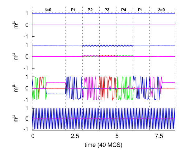
Figure 5:

References

- Amit, (1989) Amit, D. J. (1989). Modeling brain function: the world of attractor neural network. Cambridge University Press.
- Ashwin and Timme, (2005) Ashwin, P. and Timme, M. (2005). When instability makes sense. Nature, 56:36–37.
- Barrie et al., (1996) Barrie, J. M., Freeman, W. J., and Lenhart, M. (1996). Modulation by discriminative training of spatial patterns of gamma EEG amplitude and phase in neocortex of rabbits. J. Neurophysiol., 76:520–539.
- Bibitchkov et al., (2002) Bibitchkov, D., Herrmann, J. M., and Geisel, T. (2002). Pattern storage and processing in attractor networks with short-time synaptic dynamics. Network: Comput. Neural Syst., 13:115–129.
- Bolle and Vink, (1996) Bolle, D. and Vink, B. (1996). On the dynamics of analogue neurons with nonsigmoidal gain functions. Physica A, 223:293–308.
- Caroppo et al., (1999) Caroppo, D., Mannarelli, M., Nardulli, G., and Stramaglia, S. (1999). Chaos in neural networks with a nonmonotonic transfer function. Phys. Rev. E, 60:2186–2192.
- Cortes et al., (2004) Cortes, J. M., Garrido, P. L., Marro, J., and Torres, J. J. (2004). Switching between memories in neural automata with synaptic noise. Neurocomputing, 58-60:67–71.
- Cortes et al., (2006) Cortes, J. M., Torres, J. J., Marro, J., Garrido, P. L., and Kappen, H. J. (2006). Effects of fast presynaptic noise in attractor neural networks. Neural Comp., 13:614–633.
- Dominguez and Theumann, (1997) Dominguez, R. R. C. and Theumann, W. (1997). Generalization and chaos in a layered neural network. J. Phys. A: Math. Gen., 30:1403–1414.
- Faure and Korn, (2001) Faure, P. and Korn, H. (2001). Is there chaos in the brain? i. concepts of nonlinear dynamics and methods of investigation. C. R. Acad. Sci. III, 324:773–793.
- Franks et al., (2003) Franks, K. M., Stevens, C. F., and Sejnowski, T. J. (2003). Independent sources of quantal variability at single glutamatergic synapses. J. Neurosci., 23:3186–3195.
- Freeman, (2003) Freeman, W. J. (2003). Evidence from human scalp electroencephalograms of global chaotic itinerancy. Chaos, 13:1067–1077.
- Ganguly et al., (2003) Ganguly, N., Das, A., Maji, P., Sikdar, B. K., and Chaudhuri, P. P. (2003). Evolving cellular automata based associative memory for pattern recognition. In Monien, B., Prasanna, V., and Vajapeyam, S., editors, High Performance Computing - HiPC 2001 : 8th International Conference, volume 2228, pages 115–124. Springer-Verlag.
- Hansel and Sompolinsky, (1996) Hansel, D. and Sompolinsky, H. (1996). Chaos and synchrony in a model of a hypercolumn in visual cortex. J. Comput. Neurosci., 3:7–34.
- Kaneko and Tsuda, (2001) Kaneko, K. and Tsuda, I. (2001). Complex Systems: Chaos and Beyond. A Constructive Approach with Applications in Life Sciences. Springer.
- Katayama et al., (2003) Katayama, K., Sakata, Y., and Horiguchi, T. (2003). Layered neural networks with non-monotonic transfer functions. Physica A, 317:270–298.
- Kiel and Elliot, (1996) Kiel, L. D. and Elliot, E., editors (1996). Chaos Theory in the Social Sciences: Foundations and Applications. The University of Michigan Press.
- Korn and Faure, (2003) Korn, H. and Faure, P. (2003). Is there chaos in the brain? ii. experimental evidence and related models. C. R. Biol., 326:787–840.
- Lu et al., (2003) Lu, Q., Shen, G., and Yu, R. (2003). A chaotic approach to maintain the population diversity of genetic algorithm in network training. Comput. Biol. Chem., 27:363–371.
- Mainieri and Jr., (2002) Mainieri, M. and Jr., R. E. (2002). Retrieval and chaos in extremely diluted non-monotonic neural networks. Physica A, 311:581–589.
- Marro and Dickman, (1999) Marro, J. and Dickman, R. (1999). Nonequilibrium Phase Transitions in Lattice Models. Cambridge University Press.
- Pantic et al., (2002) Pantic, L., Torres, J. J., Kappen, H. J., and Gielen, S. C. A. M. (2002). Associative memory with dynamic synapses. Neural Comp., 14:2903–2923.
- Poon and Barahona, (2001) Poon, C. S. and Barahona, M. (2001). Titration of chaos with added noise. Proc. Natl. Acad. Sci. USA, 98:7107–7112.
- Rabinovich and Abarbanel, (1998) Rabinovich, M. I. and Abarbanel, H. D. I. (1998). The role of chaos in neural systems. Neuroscience, 87:5–14.
- Schweighofer et al., (2004) Schweighofer, N., Doya, K., Fukai, H., Chiron, J. V., Furukawa, T., and Kawato, M. (2004). Chaos may enhance information transmission in the inferior olive. Proc. Natl. Acad. Sci. USA, 101:4655–4660.
- Strogatz, (2003) Strogatz, S. (2003). Sync: The Emerging Science of Spontaneous Order. Hyperion, N.Y.
- Torres et al., (1997) Torres, J. J., Garrido, P. L., and Marro, J. (1997). Neural networks with fast time-variation of synapses. J. Phys. A: Math. Gen., 30:7801–7816.
- Tsodyks et al., (1998) Tsodyks, M. V., Pawelzik, K., and Markram, H. (1998). Neural networks with dynamic synapses. Neural Comp., 10:821–835.
- Tsuda, (2001) Tsuda, I. (2001). Toward an interpretation of dynamic neural activity in terms of chaotic dynamical systems. Behav. Brain Sci., 24:793–810.
- Wang et al., (1990) Wang, L., Pichler, E. E., and Ross, J. (1990). Oscillations and chaos in neural networks: An exactly solvable model. Proc. Natl. Acad. Sci. USA, 87:9467–9471.
- Zador, (1998) Zador, A. (1998). Impact of synaptic unreliability on the information transmitted by spiking neurons. J. Neurophysiol., 79:1219–1229.