Competition between synaptic depression and facilitation in attractor neural networks

Abstract

We study the effect of competition between short-term synaptic depression and facilitation on the dynamical properties of attractor neural networks, using Monte Carlo simulation and a mean field analysis. Depending on the balance between depression, facilitation and the noise, the network displays different behaviours, including associative memory and switching of the activity between different attractors. We conclude that synaptic facilitation enhances the attractor instability in a way that (i) intensifies the system adaptability to external stimuli, which is in agreement with experiments, and (ii) favours the retrieval of information with less error during short–time intervals.

1 Introduction and model

Recurrent neural networks are a prominent model for information processing and memory in the brain. (Hopfield, 1982; Amit, 1989). Traditionally, these models assume synapses that may change on the time scale of learning, but that can be assumed constant during memory retrieval. However, synapses are reported to exhibit rapid time variations, and it is likely that this finding has important implications for our understanding of the way information is processed in the brain (Abbott and Regehr, 2004). For instance, Hopfield–like networks in which synapses undergo rather generic fluctuations have been shown to significantly improve the associative process, e.g., (Marro et al., 1998). In addition, motivated by specific neurobiological observations and their theoretical interpretation (Tsodyks et al., 1998), activity–dependent synaptic changes which induce depression of the response have been considered (Pantic et al., 2002; Bibitchkov et al., 2002). It was shown that synaptic depression induces, in addition to memories as stable attractors, special sensitivity of the network to changing stimuli as well as rapid switching of the activity among the stored patterns (Pantic et al., 2002; Cortes et al., 2004; Marro et al., 2005; Torres et al., 2005; Cortes et al., 2006). This behaviour has been observed experimentally to occur during the processing of sensory information (Laurent et al., 2001; Mazor and Laurent, 2005; Marro et al., 2006).

In this paper, we present and study networks that are inspired in the observation of certain, more complex synaptic changes. That is, we assume that repeated presynaptic activation induces at short times not only depression but also facilitation of the postsynaptic potential (Thomson and Deuchars, 1994; Zucker and Regehr, 2002; Burnashev and Rozov, 2005). The question, which has not been quite addressed yet, is how a competition between depression and facilitation will affect the network performance. We here conclude that, as for the case of only depression (Pantic et al., 2002; Cortes et al., 2006), the system may exhibit up to three different phases or regimes, namely, one with standard associative memory, a disordered phase in which the network lacks this property, and an oscillatory phase in which activity switches between different memories. Depending on the balance between facilitation and depression, novel intriguing behavior results in the oscillatory regime. In particular, as the degree of facilitation increases, both the sensitivity to external stimuli is enhanced and the frequency of the oscillations increases. It then follows that facilitation allows for recovering of information with less error, at least during a short interval of time and can therefore play an important role in short–term memory processes. We are concerned in this paper with a network of binary neurons. Previous studies have shown that the behaviour of such a simple network dynamics agree qualitatively with the behaviour that is observed in more realistic networks, such as integrate and fire neuron models of pyramidal cells (Pantic et al., 2002).

Let us consider $N$ binary neurons, $s_{i}=\{1,0\},$ $i=1,...,N,$ endowed of a probabilistic dynamics, namely,

$$\mathrm{Prob}\left\{s_{i}\left(t+1\right)=1\right\}=\frac{1}{2}\left\{1+\tanh\left[2\beta h_{i}\left(t\right)\right]\right\},$$ (1)

which is controlled by a temperature parameter, $T\equiv 1/\beta;$ see, for instance, (Marro and Dickman, 2005) for details. The function $h_{i}\left(t\right)$ denotes a time–dependent local field, i.e., the total presynaptic current arriving to the postsynaptic neuron $i.$ This will be determined in the model following the phenomenological description of nonlinear synapses reported in (Markram et al., 1998; Tsodyks et al., 1998), which was shown to capture well the experimentally observed properties of neocortical connections. Accordingly, we assume that

$$h_{i}\left(t\right)=\sum_{j=1}^{N}\omega_{ij}\mathcal{D}_{j}\left(t\right)\mathcal{F}_{j}\left(t\right)s_{j}\left(t\right)-\theta_{i},$$ (2)

where $\theta_{i}$ is a constant threshold associated to the firing of neuron $i,$ and $\mathcal{D}_{j}(t)$ and $\mathcal{F}_{j}(t)$ are functions —to be determined— which describe the effect on the neuron activity of short–term synaptic depression and facilitation, respectively. We further assume that the weight $\omega_{ij}$ of the connection between the (presynaptic) neuron $j$ and the (postsynaptic) neuron $i$ are static and store a set of patterns of the network activity, namely, the familiar covariance rule:

$$\omega_{ij}=\frac{1}{Nf\left(1-f\right)}\sum_{\nu=1}^{P}\left(\xi_{i}^{\nu}-f\right)\left(\xi_{j}^{\nu}-f\right).$$ (3)

Here, $\mathrm{\xi}^{\nu}=\left\{\xi_{i}^{\nu}\right\},$ with $\nu=1\ldots,P,$ are different binary–patterns of average activity $\langle\xi_{i}^{\nu}\rangle\equiv f$. The standard Hopfield model is recovered for $\mathcal{F}_{j}=\mathcal{D}_{j}=1$, $\forall j=1,\ldots,N.$

We next implement a dynamics for $\mathcal{F}_{j}$ and $\mathcal{D}_{j}$ after the prescription in (Markram et al., 1998; Tsodyks et al., 1998). A description of varying synapses requires, at least, three local variables, say $x_{j}\left(t\right)$, $y_{j}\left(t\right)$ and $z_{j}\left(t\right),$ to be associated to the fractions of neurotransmitters in recovered, active, and inactive states, respectively. A simpler picture consists in dealing with only the $x_{j}\left(t\right)$ variable. This simplification, which seems to describe accurately both interpyramidal and pyramidal interneuron synapses, corresponds to the fact that the time in which the postsynaptic current decays is much shorter than the recovery time for synaptic depression, say $\tau_{\mathrm{rec}}$ (Markram and Tsodyks, 1996) (Time intervals are in milliseconds hereafter). Within this approach, one may write that

$$x_{j}\left(t+1\right)=x_{j}\left(t\right)+\frac{1-x_{j}\left(t\right)}{\tau_{\mathrm{rec}}}-\mathcal{D}_{j}\left(t\right)\mathcal{F}_{j}\left(t\right)s_{j}\left(t\right),$$ (4)

where

$$\mathcal{D}_{j}\left(t\right)=x_{j}\left(t\right)$$ (5)

and

$$\mathcal{F}_{j}\left(t\right)=U+\left(1-U\right)\,u_{j}\left(t\right).$$ (6)

The interpretation of this ansatz is as follows. Concerning any presynaptic neuron $j,$ the product $\mathcal{D}_{j}\mathcal{F}_{j}$ stands for the total fraction of neurotransmitters in the recovered state which are activated either by incoming spikes, $U_{j}x_{j},$ or by facilitation mechanisms, $\left(1-U_{j}\right)x_{j}u_{j};$ for simplicity, we are assuming that $U_{j}=U\in\left[0,1\right]$ $\forall j.$ The additional variable $u_{j}\left(t\right)$ is assumed to satisfy, as in the quantal model of transmitter release in (Markram et al., 1998), that

$$u_{j}\left(t+1\right)=u_{j}\left(t\right)-\frac{u_{j}\left(t\right)}{\tau_{\mathrm{fac}}}+U\left[1-u_{j}\left(t\right)\right]s_{j}\left(t\right),$$ (7)

which describes an increase with each presynaptic spike and a decay to the resting value with relaxation time $\tau_{\mathrm{fac}}$ (that is given in milliseconds) Consequently, facilitation washes out ($u_{j}\rightarrow 0,F_{j}\rightarrow U$) as $\tau_{\mathrm{fac}}\rightarrow 0,$ and each presynaptic spike uses a fraction $U$ of the available resources $x_{j}\left(t\right).$ The effect of facilitation increases with decreasing $U,$ because this will leave more neurotransmitters available to be activated by facilitation. Therefore, facilitation is not controlled only by $\tau_{\mathrm{fac}}$ but also by $U.$

The Hopfield case with static synapses is recovered after using $x_{j}=1$ in eq.(5) and $u_{j}=0$ in eq.(6) or, equivalently, $\tau_{\mathrm{rec}}=\tau_{\mathrm{fac}}=0$ in eqs. (4) and (7). In fact, the latter imply fields $h_{i}\left(t\right)=\sum_{j}\omega_{ij}Us_{j}\left(t\right)-\theta_{i},$ so that one may simply rescale both $\beta$ and the threshold.

The above interesting phenomenological description of dynamic changes has already been implemented in attractor neural networks (Pantic et al., 2002) for pure depressing synapses between excitatory pyramidal neurons (Tsodyks and Markram, 1997). We are here interested in the consequences of a competition between depression and facilitation. Therefore, we shall use $T,U,\tau_{\mathrm{rec}}$ and $\tau_{\mathrm{fac}}$ in the following as relevant control parameters.

2 Mean–field solution

Let us consider the mean activities associated, respectively, with active and inert neurons in a given pattern $\nu,$ namely,

$$m_{+}^{\nu}(t)\equiv\frac{1}{Nf}\sum_{j\in\text{Act}(\nu)}s_{j}(t),\quad m_{-}^{\nu}(t)\equiv\frac{1}{N(1-f)}\sum_{j\not\in\text{Act}(\nu)}s_{j}(t).$$ (8)

It follows for the overlap of the network activity with pattern $\nu$ that

$$m^{\nu}(t)\equiv\frac{1}{Nf\left(1-f\right)}\sum_{i}\left(\xi_{i}^{\nu}-f\right)s_{i}(t)=m_{+}^{\nu}(t)-m_{-}^{\nu}(t),$$ (9)

$\forall\nu.$ One may also define the averages of $x_{i}$ and $u_{i}$ over the sites that are active and inert, respectively, in a given pattern $\nu,$ namely,

$$\begin{array}[]{c}x_{+}^{\nu}(t)\equiv\dfrac{1}{Nf}\sum_{j\in\text{Act}(\nu)}x_{j}(t),\quad x_{-}^{\nu}(t)\equiv\dfrac{1}{N(1-f)}\sum_{j\not\in\text{Act}(\nu)}x_{j}(t)\\ u_{+}^{\nu}(t)\equiv\dfrac{1}{Nf}\sum_{j\in\text{Act}(\nu)}u_{j}(t),\quad u_{-}^{\nu}(t)\equiv\dfrac{1}{N(1-f)}\sum_{j\not\in\text{Act}(\nu)}u_{j}(t),\end{array}$$ (10)

$\forall\nu,$ which describe depression (the $x$s) and facilitation (the $u$s), each concerning a subset of neurons, e.g., $N/2$ neurons for $f=1/2.$ The local fields then ensue as

$$h_{i}(t)=\sum_{\nu=1}^{P}\left(\xi_{i}^{\nu}-f\right)M^{\nu}\left(t\right),$$ (11)

$M^{\nu}(t)\equiv\left[U+\left(1-U\right)\,u_{+}^{\nu}(t)\right]\,x_{+}^{\nu}(t)\,m_{+}^{\nu}(t)-\left[U-\left(1-U\right)\,u_{-}^{\nu}(t)\right]\,x_{-}^{\nu}(t)\,m_{-}^{\nu}(t).$

One may solve the model (1)–(7) in the thermodynamic limit $N\rightarrow\infty$ under the standard mean-field assumption that $s_{i}\approx\langle s_{i}\rangle.$ Within this approximation, we may also substitute $x_{i}$ ($u_{i}$) by the mean–field values $x_{\pm}^{\nu}$ ($u_{\pm}^{\nu}$). (Notice that one expects, and it will be confirmed below by comparisons with direct simulation results, that the mean–field approximation is accurate away from any possible critical point.) Assuming further that patterns are random with mean activity $f=1/2,$ one obtains the set of dynamic equations:

$$\qquad\quad x_{\pm}^{\nu}(t+1)=x_{\pm}^{\nu}(t)+\frac{1-x_{\pm}^{\nu}(t)}{\tau_{\mathrm{rec}}}-\left[U+\left(1-U\right)\,u_{\pm}^{\nu}(t)\,\right]\,x_{\pm}^{\nu}(t)\,m_{\pm}^{\nu}(t),$$

$$u_{\pm}^{\nu}(t+1)=u_{\pm}^{\nu}(t)-\frac{u_{\pm}^{\nu}(t)}{\tau_{\mathrm{fac}}}+U\,[1-u_{\pm}^{\nu}(t)]\,m_{\pm}^{\nu}(t),\qquad\qquad$$

$$\qquad m_{\pm}^{\nu}(t+1)=\frac{1}{N}{\sum_{i}}\left\{1\pm\tanh\left(\beta\left[M^{\nu}\left(t\right)\pm\sum_{\mu\neq\nu}\epsilon_{i}^{\mu}M^{\mu}\left(t\right)\right]\right)\right\},$$

$$m^{\nu}(t+1)=\frac{1}{N}\sum_{i}\epsilon_{i}^{\nu}\tanh\left[\beta\sum_{\mu}\epsilon_{i}^{\mu}M^{\mu}\left(t\right)\right],\qquad\qquad\qquad$$ (12)

where $\epsilon_{i}^{\mu}\equiv 2\xi_{i}^{\mu}-1.$ This is a $6P$–dimensional coupled map whose analytical treatment is difficult for large $P,$ but it may be integrated numerically, at least for not too large $P.$ One may also find the fixed–point equations for the coupled dynamics of neurons and synapses; these are

$$x_{\pm}^{\nu} = \left\{1+\,\left[U\,+\,\left(1-U\right)\,\,u_{\pm}^{\nu}\right]\,\tau_{\mathrm{rec}}\,m_{\pm}^{\nu}\right\}^{-1},$$

$$u_{\pm}^{\nu} = U\,\,\tau_{\mathrm{fac}}\,\,m_{\pm}^{\nu}\left(1\,\,+\,\,U\,\,\tau_{\mathrm{fac}}\,\,m_{\pm}^{\nu}\right)^{-1},$$

$$2m_{\pm}^{\nu} = 1\pm\frac{2}{N}{\sum_{i}}\tanh\left[\beta\left(M^{\nu}\pm\sum_{\mu\neq\nu}\epsilon_{i}^{\mu}M^{\mu}\right)\right],$$

$$m^{\nu} = \frac{1}{N}\sum_{i}\epsilon_{i}^{\nu}\tanh\left(\beta\sum_{\mu}\epsilon_{i}^{\mu}M^{\mu}\right).$$ (13)

The numerical solution of these transcendental equations describes the resulting order as a function of the relevant parameters. Determining the stability of these solutions for $\alpha=P/N\neq 0$ is a more difficult task, because it requires to linearize (12) and the dimensionality diverges in the thermodynamical limit (see however (Torres et al., 2002)). In the next section we therefore deal with the case $\alpha\rightarrow 0.$

3 Main results

Consider a finite number of stored patterns $P,$ i.e., $\alpha=P/N\rightarrow 0$ in the thermodynamic limit. In practice, it is sufficient to deal with $P=1$ to illustrate the main results (therefore, we shall suppress the index $\nu$ hereafter).

Let us define the vectors of order parameters $\vec{y}\equiv(m_{+},m_{-},x_{+},x_{-},u_{+},u_{-})$, its stationary value $\vec{y}_{st}$ that is given by the solution of Eq. 13, and $\vec{F}$ whose components are the functions on the right hand side of (12). The stability of (12) around the steady state (13) follows from the first derivative matrix $D\equiv\left(\partial\vec{F}\diagup\partial\vec{y}\right)_{\vec{y}_{\mathrm{st}}}.$ This is

$$D=\left(\begin{array}[]{cccccc}\bar{\beta}A_{+}&-\bar{\beta}A_{-}&\bar{\beta}B_{+}&-\bar{\beta}B_{-}&\bar{\beta}C_{+}&-\bar{\beta}C_{-}\\ -\bar{\beta}A_{+}&\bar{\beta}A_{-}&-\bar{\beta}B_{+}&\bar{\beta}B_{-}&-\bar{\beta}C_{+}&\bar{\beta}C_{-}\\ -A_{+}&0&\tau-B_{+}&0&-C_{+}&0\\ 0&-A_{-}&0&\tau-B_{-}&0&-C_{-}\\ D_{+}&0&0&0&\tau-E_{+}&0\\ 0&D_{-}&0&0&0&\tau-E_{-}\end{array}\right)$$ (14)

where $\bar{\beta}\equiv 2\beta m_{+}m_{-},$ $A_{\pm}\equiv\left[U+\left(1-U\right)\,u_{\pm}\right]\,x_{\pm},$ $B_{\pm}\equiv\left[U+\left(1-U\right)\,u_{\pm}\right]\,m_{\pm},$ $C_{\pm}\equiv\left(1-U\right)\,x_{\pm}m_{\pm},$ $D_{\pm}\equiv U(1-u_{\pm}),$ $\tau\equiv 1-\tau_{\mathrm{rec}}^{-1},$ and $E_{\pm}\equiv Um_{\pm}.$ After noticing that $m_{+}+m_{-}=1,$ one may numerically diagonalize $D$ and obtain the eigenvalues $\lambda_{n}$ for a given set of control parameters $T,U,\tau_{\mathrm{rec}},\tau_{\mathrm{fac}}.$ For $\left|\lambda_{n}\right|<1$ $(\left|\lambda_{n}\right|>1),$ the system is stable (unstable) close to the fixed point $y_{n}$. The maximum of $\left|\lambda_{n}\right|$ determines the local stability: for $\left|\lambda_{n}\right|_{\mathrm{max}}<1,$ the system (12) is locally stable, while for $\left|\lambda_{n}\right|_{\mathrm{max}}>1$ there is at least one direction of instability, and the system consequently becomes locally unstable. Therefore, varying the control parameters one crosses the line $|\lambda|_{\mathrm{max}}=1$ that signals the bifurcation points.

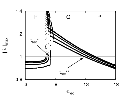
Figure 1: The three relevant regions, denoted F, O and P, respectively, that are depicted by the absolute value of the maximum eigenvalue $\left|\lambda_{n}\right|_{\mathrm{max}}$ of the stability matrix $D$ in (14) when plotted as a function of the recovering time $\tau_{\mathrm{rec}}$ for different values of the facilitation time $\tau_{\mathrm{fac}}.$ Here, $\tau_{\mathrm{fac}}=10,$ 15, 20 and 25 for different curves from bottom to top, respectively, in the F and P regions. The stationary solutions lack of any local stability for $\tau_{\mathrm{rec}}^{\ast}<\tau_{\mathrm{rec}}<\tau_{\mathrm{rec}}^{\ast\ast}$ (O), and the network activity then undergoes oscillations. The arrows signal $\tau_{\mathrm{rec}}^{\ast}$ and $\tau_{\mathrm{rec}}^{\ast\ast}$ for $\tau_{\mathrm{fac}}=10.$ This graph is for $U=0.1$ and $T=0.1.$

Figure 2: This illustrates how the different regimes of the network activity depend on the balance between depression and facilitation. Top graphs: Phase diagram ($\tau_{\mathrm{rec}},\tau_{\mathrm{fac}}$) for $\alpha=0$ and $U=0.1$ at temperature $T=0.1$ (left) and $0.05$ (right). The dashed (solid) line is for $\tau_{\mathrm{rec}}^{\ast}$ ($\tau_{\mathrm{rec}}^{\ast\ast}$) signaling the first–order (second–order) phase transitions between the O and F(P) phases. The insets show the resulting width of the oscillatory region, $\delta\equiv\tau_{\text{rec}}^{\ast\ast}-\tau_{\text{rec}}^{\ast},$ as a function of $\tau_{\mathrm{fac}}.$ Bottom graphs: Phase diagram ($\tau_{\mathrm{rec}},U$) for $\alpha=0$ and $T=0.1,$ and $\gamma\equiv\tau_{\mathrm{fac}}/\tau_{\mathrm{rec}}=1$ (left) and $0.25$ (right).

The resulting situation is summarized in figure 1 for specific values of $U,$ $T$ and $\tau_{\mathrm{fac}},$. Eqs. (13) have three solutions, two of which are memory states corresponding to the pattern and anti-pattern and the other a so-called paramagnetic state that has no overlap with the memory pattern. The stability of the two solutions depends on $\tau_{\mathrm{rec}}$. The region $\tau_{\mathrm{rec}}>\tau_{rec}^{\ast\ast}$ corresponds to the non-retrieval phase, where the paramagnetic solution is stable and the memory solutions are unstable. In this phase, the average network behaviour has no significant overlap with the stored memory pattern. The region $\tau_{\mathrm{rec}}<\tau_{\mathrm{rec}}^{*}$ corresponds to the memory phase, where the paramagnetic solution is unstable and the memory solutions are stable. The network retrieves one of the stored memory patterns. For $\tau_{\mathrm{rec}}^{\ast}<\tau_{\mathrm{rec}}<\tau_{\mathrm{rec}}^{\ast\ast}$ (denoted “O” in the figure) none of the solutions is stable. The activity of the network in this regime keeps moving from one to the other fixed–points neighborhood (the pattern and anti-pattern in this simple example). This rapid switching behaviour is typical for dynamical synapses and does not occur for static synapses. A similar oscillatory behavior was reported in (Pantic et al., 2002; Cortes et al., 2004) for the case of only synaptic depression. A main novelty is that the inclusion of facilitation importantly modifies the phase diagram, as discussed below (figure 2). On the other hand, the phases for $\tau_{\mathrm{rec}}<\tau_{\mathrm{rec}}^{\ast}$ (F) and $\tau_{\mathrm{rec}}>\tau_{\mathrm{rec}}^{\ast\ast}$ (P) correspond, respectively, to a locally–stable regime with associative memory ($m\neq 0$) and to a disordered regime without memory (i.e., $m\equiv m^{1}=0$).

The values $\tau_{\mathrm{rec}}^{\ast}$ and $\tau_{\mathrm{rec}}^{\ast\ast}$ which, as a function of $\tau_{\mathrm{fac}},$ $U$ and $T,$ determine the limits of the oscillatory phase correspond to the onset of condition $|\lambda_{n}|_{\mathrm{max}}>1.$ This condition defines lines in the parameter space ($\tau_{\text{rec}},\tau_{\text{fac}}$) that are illustrated in figure 2. This reveals that $\tau_{\text{rec}}^{\ast}$ (separation between the F and O regions) in general decreases with increasing facilitation, which implies a larger oscillatory region and consequently a reduction of the memory phase. On the other hand, $\tau_{\text{rec}}^{\ast\ast}$ (separation between O and P regions) in general increases with facilitation, thus broadening further the width of the oscillatory phase $\delta\equiv\tau_{\text{rec}}^{\ast\ast}-\tau_{\text{rec}}^{\ast}.$ The behavior of this quantity under different conditions is illustrated in the insets of figure 2.

Another interesting consequence of facilitation are the changes in the phase diagram as one varies the facilitation parameter $U$ which measures the fraction of neurotransmitter that are not activated by the facilitating mechanism. In order to discuss this, we define the ratio between the time scales, $\gamma\equiv\tau_{\mathrm{fac}}/\tau_{\mathrm{rec}},$ and monitor the phase diagram ($\tau_{\mathrm{rec}},U$) for varying $\gamma.$ The result is also in figure 2 —see the bottom graphs for $\gamma=1$ (left) and $0.25$ (right) which correspond, respectively, to a situation in which depression and facilitation occur in the same time scale and to a situation in which facilitation is four times faster. The two cases exhibit a similar behavior for large $U,$ but they are qualitatively different for small $U.$ In the case of faster facilitation, there is a range of $U$ values for which $\tau_{\text{rec}}^{\ast}$ increases, in such a way that one passes from the oscillatory to the memory phase by slightly increasing $U.$ This means that facilitation tries to drive the network activity to one of the attractors ($\tau_{\mathrm{fac}}<\tau_{\mathrm{rec}}$) and, for weak depression ($U$ small), the activity will remain there. Decreasing $U$ further has then the effect of increasing effectively the system temperature, which destabilizes the attractor. This only requires small $U$ because the dynamics (7) rapidly decreases the second term in $\mathcal{F}_{j}$ to zero.

Figure 3: For $U=T=0.1$ as in figure 1, these graphs illustrate results from Monte Carlo simulations (symbols) and mean–field solutions (curves) for the case of associative memory under competition of depression and facilitation. This shows $m\equiv m^{1}$ as a function of $\tau_{\mathrm{rec}}$ (horizontal axis) and $\tau_{\mathrm{fact}}$ (different curves as indicated) corresponding to regimes in which the limiting value $\tau_{\mathrm{rec}}^{\ast}$ decreases (left graph) or increases (right graph) with increasing $\tau_{\mathrm{fac}},$ the two situations that are discussed in the main text.

Figure 3 shows the variation with both $\tau_{\mathrm{rec}}$ and $\tau_{\mathrm{fac}}$ of the stationary locally–stable solution with associative memory, $m\neq 0$, computed this time both in the mean field approximation and using Monte Carlo simulation. This Monte Carlo simulation consists of iterating eqs. (1), (4) and (7) using parallel dynamics. This shows a perfect agreement between our mean–field approach above and Monte Carlo simulations as long as one is far from the transition, a fact which is confirmed below (in figure 5). This is because, near $\tau_{\mathrm{rec}}^{\ast},$ the simulations describe hops between positive and negative $m$ which do not compare well with the mean–field absolute value $\left|m\right|.$

Figure 4: Phase diagram $(T,\tau_{\mathrm{fac}})$ for $U=0.1$ and $\tau_{\mathrm{rec}}=3$ms. This illustrates the potential high adaptability of the network to different tasks, e.g., around $T=0.22,$ by simply varying its degree of facilitation.

The most interesting behavior is perhaps the one revealed by the phase diagram $(T,\tau_{\mathrm{fac}})$ in figure 4. Here we depict a case with $U=0.1,$ in order to clearly visualize the effect of facilitation —facilitation has practically no effect for any $U>0.5,$ as shown above— and $\tau_{\mathrm{rec}}=3$ms in order to compare with the situation of only depression in Pantic et al. (2002). A main result here is that, for appropriate values of the working temperature $T$, one may force the system to undergo different types of transitions by simply varying $\tau_{\mathrm{fac}}.$ First note, that the line $\tau_{\mathrm{fac}}=0$ corresponds roughly to the case of static synapses, since $\tau_{\mathrm{rec}}$ is very small. In this limit the transition between retrieval (F) and non-retrieval (P) phases is at $T=U=0.1$ At low enough $T,$ there is transition between the non–retrieval (P) and retrieval phases (F) as facilitation is increased. This reveals a positive effect of facilitation on memory at low temperature, and suggests improvement of the network storage capacity which is usually measured at $T=0,$ a prediction that we have confirmed in preliminary simulations. At intermediate temperatures, e.g., $T\approx 0.22$ for $U=0.1,$ the systems shows no memory in the absence of facilitation, but increasing $\tau_{\mathrm{fac}}$ one may describe consecutive transitions to a retrieval phase (F), to a disordered phase (P), and then to an oscillatory phase (O). The latter is associated to a new instability induced by a strong depression effect due to the further increase of facilitation. At higher $T,$ facilitation may drive the system directly from complete disorder to an oscillatory regime.

Figure 5: Left graph: Half period of oscillations as a function of $\tau_{\text{fac}}$, for $\tau_{\text{rec}}=10,$ $U=T=0.1$ and $P=1,$ as obtained from the mean–field solution (solid curve) and from simulations (symbols). Right graph: For the same conditions than in the left graph, this shows the maximum of the absolute value of $m$ during oscillations. The simulation results in both graphs correspond to an average over $10^{3}$ peaks of the stationary series for $m$. The fact the statistical errors are small confirms a periodic behavior.

In addition to its influence on the onset and width of the oscillatory region, $\tau_{\text{fac}}$ determines the frequency of the oscillations of $m.$ In order to study this effect, we computed the average time between consecutive minimum and maximum of these oscillations, i.e., a half period. The result is illustrated in the left graph of figure 5. This shows that the frequency of the oscillations increases with the facilitation time. This means that the access of the network activity to the attractors is faster with increasing facilitation, though the system then remains a shorter time near each attractor due to an stronger depression. On the other hand, we also computed the maximum of $m$ during oscillations, namely, $|m|_{\mathrm{max}}.$ This, which is depicted in the right graph of figure 5, also increases with $\tau_{\text{fac}}.$ The overall conclusion is that not only the access to the stored information is faster under facilitation but that increasing facilitation will also help to retrieve information with less error.

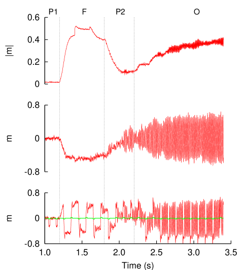
Figure 6: Time series for the overlap function, $m,$ at $T=0.22$ (horizontal dotted line in figure 4) as one increases the value of $\tau_{\text{fac}}$ in order to visit the different regimes (separated here by vertical lines). The simulations started with $\tau_{\text{fac}}=1$ at $t=1$ and $\tau_{\text{fac}}$ was then increased by 10 units every 200 ms. The bottom graph corresponds to a case in which the system is under the action of an external stimulus (as described in the main text). The middle graph depicts an individual run when the system is without any stimulus, and the top graph corresponds to the average of $\left|m\right|$ over 100 independent runs of the unperturbed system.

In order to deepen further on some aspects of the system behavior, we present in figures 6 and 7 a detailed study of specific time series. The middle graph in figure 6 corresponds to a simulation of the system evolution for increasing values of $\tau_{\text{fac}}$ as one describes the horizontal line for $T=0.22$ in figure 4. The system thus visits consecutively the different regions (separated by vertical lines) as time goes on. That is, the simulation starts with the system in the stable paramagnetic phase, denoted P1 in the figure, and then successively moves by varying $\tau_{\text{fac}}$ into the stable ferromagnetic phase F, into another paramagnetic phase, P2, and, finally, into the oscillatory phase O.

We interpret that the observed behavior in P2 is due to competition between the facilitation mechanism, which tries to bring the system to the fixed–point attractors, and the depression mechanism, which tends to desestabilize the attractors. The result is a sort of intermittent behavior in which oscillations and convergence to a fixed point alternates, in a way which resembles (but is not) chaos. The top graph in figure 6, which corresponds to an average over independent runs, illustrates the typical behaviour of the system in these simulations; the middle run depicts an individual run.

Further interesting behavior is shown in the bottom graph of figure 6. This corresponds to an individual run in the presence of a very small and irregular external stimulus which is represented by the (green) line around $m=0.$ This consist of an irregular series of positive and negative pulses of intensity $\pm 0.03\xi^{1}$ and duration of 20 ms. In addition to a great sensibility to weak inputs from the environment, this reveals that increasing facilitation tends to significantly enhance the system response.

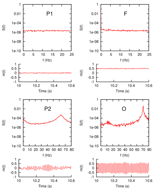
Figure 7: Spectral analysis of the cases in figure 6. On top of each of the small panels, which show typical time series for $\tau_{\text{fac}}=2,$ 20, 50 and 100, respectively, from top to bottom and from left to right, the square panels show the corresponding power spectra. Details of the simulations as in figure 6.

Figure 7 shows the power spectra of typical time series such as the ones in figure 6, namely, describing the horizontal line for $T=0.22$ in figure 4 to visit the different regimes. We plot here time series $m\left(t\right)$ obtained, respectively, for $\tau_{\text{fac}}=2,$ 20, 50 and 100 and, on top of each of them, the corresponding spectra. This reveals a flat, white–noise spectra for the P1 phase and also for the stable fixed–point solution in the F regime. However, the case for the intermittent P2 phase depicts a small peak around 65 Hz. The peak is much sharper and it occurs at 70 Hz in the oscillatory case.

4 Conclusion

We have shown that the dynamical properties of synapses have profound consequences on the behaviour, and the possible functional role, of recurrent neural networks. Depending on the relative strength of the depression, the facilitation and the noise in the network, one observes attractor dynamics to one of the stored patterns, non-retrieval where the neurons fire largely at random in a fashion that is uncorrelated to the stored memory patterns, or switching where none of the stored patterns is stable and the network switches rapidly between (the neighborhoods of) all of them. These three behaviours were also observed in our previous work where we studied the role of depression.

The particular role of facilitation is the following. The transitions between these possible phases are controlled by two facilitation parameters, namely, $\tau_{\mathrm{fac}}$ and $U.$ Analysis of the oscillatory phase reveals that the frequency of the oscillations, as well as the maximum retrieval during oscillations increase when the degree of facilitation increases. That is, facilitation favours in the model a faster access to the stored information with a noticeably smaller error. This suggests that synaptic facilitation might have an important role in short–term memory processes.

There is increasing evidence in the literature that similar jumping processes could be at the origin of the animals ability to adapt and rapidly response to the continuously changing stimuli in their environment. We therefore believe that the network behaviour that is the consequence of dynamic synapses as presented in this paper may have important functional implications.

References

- Abbott and Regehr (2004) L. F. Abbott and W. G. Regehr. Synaptic computation. Nature, 431:796–803, 2004.
- Amit (1989) D. J. Amit. Modeling brain function: The world of attractor neural networks. Cambridge University Press, 1989.
- Bibitchkov et al. (2002) D. Bibitchkov, J. M. Herrmann, and T. Geisel. Pattern storage and processing in attractor networks with short-time synaptic dynamics. Network: Comput. Neural Syst., 13:115–129, 2002.
- Burnashev and Rozov (2005) N. Burnashev and A. Rozov. Presynaptic Ca2+ dynamics, Ca2+ buffers and synaptic efficacy. Cell Calcium, 37:489–495, 2005.
- Cortes et al. (2004) J. M. Cortes, P. L. Garrido, J. Marro, and J. J. Torres. Switching between memories in neural automata with synaptic noise. Neurocomputing, 58-60:67–71, 2004.
- Cortes et al. (2006) J. M. Cortes, J. J. Torres, J. Marro, P. L. Garrido, and H. J. Kappen. Effects of Fast Presynaptic Noise in Attractor Neural Networks. Neural Comp., 18(3):614–633, 2006.
- Hopfield (1982) J. J. Hopfield. Neural Networks and Physical Systems with Emergent Collective Computational Abilities. Proc. Natl. Acad. Sci. USA, 79:2554–2558, 1982.
- Laurent et al. (2001) G. Laurent, M. Stopfer, R. W. Friedrich, M. I. Rabinovich, A. Volkovskii, and H. D. I. Abarbanel. Odor encoding as an active, dynamical process: experiments, computation and theory. Annu. Rev. Neurosci., 24:263–297, 2001.
- Markram and Tsodyks (1996) H. H. Markram and M. V. Tsodyks. Redistribution of synaptic efficacy between pyramidal neurons Nature, 382:807–810, 1996.
- Markram et al. (1998) H. H. Markram, Y. Wang, and M. V. Tsodyks. Differential signaling via the same axon of neocortical pyramidal neurons. Proc. Natl. Acad. Sci. USA, 95:5323–5328, 1998.
- Marro and Dickman (2005) J. Marro and R. Dickman. Nonequilibrium phase transitions in lattice models. Cambridge University Press, 2005.
- Marro et al. (1998) J. Marro, P. L. Garrido, and J. J. Torres. Effect of correlated fluctuations of synapses in the performance of neural networks. Phys. Rev. Lett., 81:2827–2830, 1998.
- Marro et al. (2005) J. Marro, J. J. Torres, and J. M. Cortes. Chaotic hopping between attractors in neural automata. Submitted, 2005.
- Marro et al. (2006) J. Marro, J. J. Torres, J. M. Cortes, B. Wemmenhove, and H. J. Kappen. Sensitivity, itinerancy and chaos in partly–synchronized weighted networks. To be published, 2006.
- Mazor and Laurent (2005) O. Mazor and G. Laurent. Transient Dynamics versus Fixed Points in Odor Representations by Locust Antennal Lobe Projection Neurons. Neuron, 48:661–673, 2005.
- Pantic et al. (2002) L. Pantic, J. J. Torres, H. J. Kappen, and S. C. A. M. Gielen. Associative Memory with Dynamic Synapses. Neural Comp., 14:2903–2923, 2002.
- Thomson and Deuchars (1994) A. M. Thomson and J. Deuchars. Temporal and spatial properties of local circuits in neocortex. Trends Neurosci., 17:119–126, 1994.
- Torres et al. (2005) J. J. Torres, J. Marro, P. L. Garrido, J. M. Cortes, F. Ramos, and M. A. Munoz. Effects of static and dynamic disorder on the performance of neural automata. Biophysical Chemistry, 115:285–288, 2005.
- Torres et al. (2002) J. J. Torres, L. Pantic, and H. J. Kappen. Storage capacity of attractor neural networks with depressing synapses. Phys. Rev. E., 66:061910, 2002.
- Tsodyks et al. (1998) M. Tsodyks, K. Pawelzik, and H. Markram. Neural networks with dynamic synapses. Neural Comp., 10:821–835, 1998.
- Tsodyks and Markram (1997) M. V. Tsodyks and H. H. Markram. The neural code between neocortical pyramidal neurons depends on neurotransmitter release probability. Proc. Natl. Acad. Sci. USA, 94:719–723, 1997.
- Zucker and Regehr (2002) R.S. Zucker and W. G. Regehr. Short–time synaptic plasticity. Annu. Rev. Physiol., 64:355–405, 2002.