Solitons in Yakushevich-like models of DNA dynamics with improved intrapair potential

Summary. The Yakushevich model provides a very simple pictures of DNA torsion dynamics, yet yields remarkably correct predictions on certain physical characteristics of the dynamics. In the standard Yakushevich model, the interaction between bases of a pair is modelled by a harmonic potential, which becomes anharmonic when described in terms of the rotation angles; here we substitute to this different types of improved potentials, providing a more physical description of the H-bond mediated interactions between the bases. We focus in particular on soliton solutions; the Yakushevich model predicts the correct size of the nonlinear excitations supposed to model the “transcription bubbles”, and this is essentially unchanged with the improved potential. Other features of soliton dynamics, in particular curvature of soliton field configurations and the Peierls-Nabarro barrier, are instead significantly changed.

Introduction

In the DNA transcription process, a specialized enzyme (RNA-Polymerase) binds to a specific site of the DNA double helix and unwinds it in a local region of 15-20 bases, thus creating a “transcription bubble”; the RNAP and the bubble travel then along the DNA, copying its sequence and producing a RNA-Messenger to be later used to express genes or replicate the local sequence.

This process requires a very finely tuned coordination of the motion of RNAP – and production of the RNA-Messenger – with the dynamics of the DNA double chain. In a pioneering paper appeared in 1980, Englander, Kallenbach, Heeger, Krumhansl and Litwin [8] suggested that nonlinear excitations in the DNA double chain could be instrumental in this process and allow the motion of the transcription bubble to occur at near-zero energy cost.

In particular, as the fundamental motion undergone by DNA nucleotides in this process is a roto/torsional one, they suggested to model the DNA molecule as a double chain of coupled pendulums; the relevant nonlinear excitations would then be (topological) solitons pretty much like those well known in the sine-Gordon equation. We refer to their work for detail.

Their suggestion was taken up by a number of author, producing several variants of their fundamental model (these are reviewed in [25], to which the reader is referred for detail and discussion). In particular, a simple model was put forward by L.V. Yakushevich [23], see also [24, 25, 26] for further results and extensions; this is recalled and discussed in sect.1 below.

The Yakushevich (Y) model has its appeal, and at the same time weakness, in its simplicity; it is remarkable that despite such simplicity it predicts correct orders of magnitude for a number of physical features, such as timescales of small oscillations and – most relevant in the wake of the approach of Englander et al. – size of the nonlinear excitations: in fact, this corresponds to the experimental size of the transcription bubble.

At the same time, the Yakushevich model is a first-grade (i.e. one degree of freedom per nucleotide [24]), idealized (i.e. DNA is considered as a homogeneous chain [24]), and nearly-linear model: interaction between successive nucleotides is via a harmonic potential, and the intrapair interaction (i.e. interaction between bases in a Watson-Crick pair, and though these between the corresponding nucleotides) is also modelled by a potential which is harmonic in the distance, and becomes anharmonic when described in terms of the relevant degrees of freedom, i.e. rotation angles.

While the first two features are nearly unavoidable (but see [20]) in models to be analyzed in analytical – and not just numerical – terms, near-linearity raises more perplexity even from the point of view of a mathematical approach, in particular since the motions we are mainly interested in are fully nonlinear.

In this note we consider a modified Y model, in which the intrapair potential is no longer near-linear. Our main motivation in this study was to understand how much of the prediction of Y model survives a fully nonlinear modelling of the intrapair potential. Note in this respect that the Peyrard-Bishop (PB) model [19] considers a fully nonlinear Morse potential for this interaction. In this case we should also consider the directionality of H bonding, which plays no role in the “straight” motions considered in the PB model and is not taken into account by the Morse-PB potential.

More radical modifications of the standard Yakushevich model, modifying the other features mentioned above, could also be considered; these will be studied elsewhere [3].

As the interaction between bases in a pair is mediated by H bonds, we argue that a more realistic approximation is that of a potential describing H-bond interactions. This could be a Morse potential as in the PB model, better if modified by taking into account directionality effects; or even – as we will do in the first instance – given that H bonds results from essentially dipolar forces, a dipole-dipole interaction. This is not entirely correct, since as bases rotate the charge distribution is also modified, but takes into account several features of H bonding, in particular its directionality, and of the motion geometry, which are not considered in the standard Y model. In a way, the dipole-dipole potential tests an approximation which is orthogonal to the one represented by the Yakushevich potential.

It should be mentioned that this work continues investigation described in [13], where we considered how the nonlinear dynamics of the Y model is affected by dropping the contact approximation $\ell_{0}=0$; as in the present case, we have shown there that albeit the linear dynamics of the Y model is strongly affected by the approximations this model assumes, the physical features of fully nonlinear excitations are remarkably robust i.e. survive when we drop those approximations (that of $\ell_{0}=0$ in [13], that of a harmonic intrapair potential here). The same does not hold when one touches other features of the model, as will be shown in forthcoming work [3, 20].

In the following, after describing the standard Y model, including also “helicoidal” terms [5, 9] (sect.1), we discuss in some detail the case of general Y-like models and in particular the reduced equations describing soliton solutions (sect.2). These equations depend on the intrapair potential $V$ modelling H-bond interactions; we also focus on the special case of soliton solutions of topological indices (1,0) and (0,1), see below for definitions. In sections 3–5 we consider different cases for the intrapair potential: the dipole-dipole potential in sect.3, the Morse-PB potential in sect.4, and a Morse potential modified by introducing a directional term in sect.5. In all cases, we use the detailed discussion of sect.2 and tackle directly the effective equations obtained there; these provide a description of the special soliton equations which can be compared – as we do – with those provided by the standard Y model. All this discussion is conducted on continuous models, but the DNA chain is intrinsically discrete; in sect.6 we evaluate numerically a relevant parameter providing some measure of the relevance of discreteness effects, i.e. the height of the Peierls-Nabarro barrier. The final sect.7 is devoted to a discussion of the results obtained and to drawing some conclusions.

Acknowledgements

This work received support by the Italian MIUR (Ministero dell’Istruzione, Università e Ricerca) under the program COFIN2004, as part of the PRIN project “Mathematical Models for DNA Dynamics ($M^{2}\times D^{2}$)”. I would like to thank M. Cadoni, R. De Leo and G. Saccomandi for useful discussions.

1 Yakushevich model

The Yakushevich model (Y model) is an “ideal” DNA model [25]. That is, the DNA double chain is considered to be of infinite length, and all bases are considered as being equal.

In the Yakushevich model, each nucleotide is considered as a single unit, and its state described in terms of an angular variable. That is, each nucleotide is seen as a rigid disk of radius $r$ which can rotate around an axis and has a moment of inertia $I$ around this axis; the rotation of the nucleotide at site $i\in{\bf Z}$ on the chain $a$ ($a=1,2$) is described by an angle $\vartheta^{(a)}_{i}$. When we are referring to a specific base pair, we write simply $\vartheta_{1},\vartheta_{2}$ for $\vartheta^{(1)}_{i},\vartheta^{(2)}_{i}$. The axes of rotation of the two disks lie a distance $A\geq r$ away.

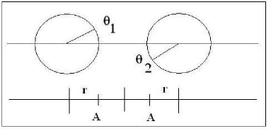
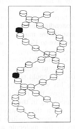
Figure 1: Left: A base pair in the Yakushevich model. Nucleotides are represented as disks of radius $r$; here $A=r+\ell_{0}/2$ is the distance between the centers of disks and the axis of the double helix. Right: Bases which are half-pitch of the helix away and on opposite chains are actually near enough in space, and Bernal-Fowler filaments [6] joining them can form; they mediate the “helicoidal interactions” described by (1.3).

The model is better described by a Lagrangian $L=T-U$. In this, the kinetic energy is obviously given by

$$T\ =\ \sum_{a}\,\sum_{i}{I\over 2}\,({\dot{\vartheta}}^{(a)}_{i})^{2}\ .$$

The potential energy $U$ is the sum of two terms, or three if we consider the so-called “helicoidal” version of the model [5, 9, 25]. These are the stacking ($U_{s}$) term, the pairing one $(U_{p}$), and maybe the helicoidal one $U_{h}$; the latter is relevant only in small amplitude dynamics and in the dispersion relations. Thus

$$U\ =\ U_{s}\,+\,U_{h}\,+\,U_{p}\ .$$

The first two terms correspond to harmonic potentials and depend on dimensional coupling constants $K_{s}$ and $K_{h}$. The first, describing backbone torsion and stacking interactions between bases at nearby sites on the same chain, is given by

$$U_{s}\ =\ {K_{s}\over 2}\ \sum_{a}\,\sum_{i}\,\left(\vartheta^{(a)}_{i+1}-\vartheta^{(a)}_{i}\right)^{2}\ .$$

The helicoidal term describes interactions between bases which are nearby in space due to helical geometry, and mediated in real DNA by Bernal-Fowler filaments (chains of hydrogen bonded water molecules [6]), which join a base and the one on the other chain half-pitch of the helix away, see fig.1b; in B-DNA, this means a distance of $h=5$ sites along the DNA double chain. These are very weak interactions, and are also modelled by a harmonic potential:

$$U_{h}\ =\ {K_{s}\over 2}\ \sum_{a}\,\sum_{i}\,\left(\vartheta^{(\widehat{a})}_{i+h}-\vartheta^{(a)}_{i}\right)^{2}\ .$$

This term has no effect on fully nonlinear dynamics [14], but introduces qualitative changes in small amplitude dynamics and dispersion relations; we will thus drop it when considering fully nonlinear excitations.

As for the $U_{p}$ term, it describes the nonlinear interactions between bases in a pair, i.e.

$$U_{p}\ =\ \sum_{i}\ V(\vartheta^{(1)}_{i},\vartheta^{(2)}_{i})$$

with $V$ the intrapair potential.

We will call the models of the class described so far, with general $V$, Yakushevich -like models; we denote the original Yakushevich model (with $V$ given by (1.5) below) as the “standard” Y-model.

In the standard Y model it is assumed that

$$V\ =\ (1/2)\,K_{p}\ (\ell-\ell_{0})^{2}\ ,$$

where $\ell$ is the distance between the atoms bridged by the H bonds, and $\ell_{0}$ is this distance in the equilibrium configuration described by $\vartheta^{(a)}_{i}=0$. Note $r+\ell_{0}/2=A$.

This harmonic potential becomes anharmonic in terms of the angles $\vartheta^{(a)}_{i}$. Indeed, with simple algebra (and writing, for ease of notation, $\vartheta_{a}$ for $\vartheta^{(a)}_{i}$) we have $\ell^{2}=(\ell_{0}^{2}+4\ell_{0}r+6r^{2})-2r(\ell_{0}+2r)[\cos\vartheta_{1}+\cos\vartheta_{2}]+2r^{2}\cos(\vartheta_{1}-\vartheta_{2})$.

In the usual treatments of the Y model, one considers the approximation $\ell_{0}=0$, also called “contact approximation” (a discussion of the usual Y model beyond the contact approximation is given in [13]). With this, $r\simeq A$ and

$$(\ell-\ell_{0})^{2}\ =\ \ell^{2}\ =\ 2r^{2}[3-2(\cos(\vartheta_{1})+\cos(\vartheta_{2}))+\cos(\vartheta_{1}-\vartheta_{2})]\ ;$$

expanding around the equilibrium we get $\ell^{2}\approx r^{2}(\vartheta_{1}+\vartheta_{2})^{2}$. Thus,

$$V\ =\ K_{p}r^{2}\ \left[\cos(\vartheta^{(1)}_{i}-\vartheta^{(2)}_{i})-2\,\left(\cos\vartheta^{(1)}_{i}+\cos\vartheta^{(2)}_{i}\right)+3\right]\ .$$

The intrapair potential term $U_{p}$ reads from this and (1.4). This completes the description of the Yakushevich model..

In studying the Y model it is convenient to pass to variables

$$\psi_{n}=\left(\vartheta^{(1)}_{n}+\vartheta^{(2)}_{n}\right)/2\ ,\ \chi_{n}=\left(\vartheta^{(1)}_{n}-\vartheta^{(2)}_{n}\right)/2$$

(thus $\vartheta^{(1)}_{n}=\psi_{n}+\chi_{n}$ and $\vartheta^{(2)}_{n}=\psi_{n}-\chi_{n}$), and introduce

$$a=K_{s}/I\ ,\ b=K_{h}/I\ ,\ c=2r^{2}(K_{p}/I)\ .$$

The Euler-Lagrange equations stemming from the Yakushevich Lagrangian are

$$\begin{array}[]{rl}{\ddot{\psi}}_{n}\ =&\ a\,(\psi_{n+1}-2\psi_{n}+\psi_{n-1})\ +\ b(\psi_{n+h}-2\psi_{n}+\psi_{n-h})\ +\\ &\ -\ c\,\sin\psi\,\cos\chi\ ,\\ {\ddot{\chi}}_{n}\ =&\ a\,(\chi_{n+1}-2\chi_{n}+\chi_{n-1})\ -\ b(\chi_{n+h}+2\chi_{n}+\chi_{n-h})\ +\\ &\ -\ c\,\sin\chi\,\left(\cos\psi-\cos\chi\right)\ .\end{array}$$

Linearizing these about the equilibrium $\psi_{n}=\chi_{n}=0$ and writing $\psi_{n}=f_{q\omega}\exp[i(qn+\omega t)]$, $\chi_{n}=g_{q\omega}\exp[i(qn+\omega t)]$, $q=k\delta$, yields the dispersion relations

$$\begin{array}[]{l}\omega^{2}_{\psi}\ =\ 2a\,(1-\cos(k\delta))\ +\ 2b(1-\cos(k\delta h))\ +\ c\ ;\\ \omega^{2}_{\chi}\ =\ 2a\,(1-\cos(k\delta))\ +\ 2b(1+\cos(k\delta h))\ .\end{array}$$

As for the dimensional parameters appearing in the model, we adopt those suggested in [12], i.e.

$$\begin{array}[]{c}r=A=5.5\,{\rm\AA}\ ,\ \ \delta=3.4\,{\rm\AA}\ ;\ \ I=3\cdot 10^{-37}{\rm cm}^{2}\cdot{\rm g}\ ;\\ K_{s}=0.13{\rm eV/rad}^{2}\ ,\ K_{p}r^{2}=0.025{\rm eV/rad}^{2}\ ,\ K_{h}=0.009{\rm eV/rad}^{2}\ .\end{array}$$

The choice for $K_{p}$ corresponds to an energy of $0.1{\rm eV}$ for the breaking of the intrapair coupling (this is $\Delta E=V(\pi,\pi)-V(0,0)$); this corresponds to 2.5 times the energy needed for breaking a H bond, i.e. is intermediate between the A-T and the G-C cases.

The full equations admit travelling wave solutions; these are better discussed in the continuum approximation in which the arrays $\{\vartheta^{(1)}_{i},\vartheta^{(2)}_{i}\}$, and hence $\{\psi_{i}(t)\}$ and $\{\chi_{i}(t)\}$, are promoted to fields $\vartheta_{a}(x,t)$, $\phi(x,t)$, $\xi(x,t)$. The finite energy condition require that each $\vartheta_{a}(x,t)$ goes to a multiple of $2\pi$ (with vanishing $x$ derivative) for $|x|\to\infty$; hence finite energy travelling wave solutions are indexed by two integer rotation numbers $(m,n)$. It turns out that there is a maximum speed $v_{0}=\sqrt{a}\delta$ for these.

The fundamental soliton solutions can be easily determined analytically. They are given, respectively, by

$$\begin{array}[]{ll}\varphi(z)\ =\ 4\,{\rm arctan}[e^{\kappa z}]\ ,&\ \xi=0\ ;\\ \xi(z)\ =\ 2\,{\rm arccos}\left({-\kappa z/\sqrt{1+\kappa^{2}z^{2}}}\right)\ ,&\varphi=0\ .\end{array}$$

Here we have written $\kappa:=\sqrt{c/(a\delta^{2}-Iv^{2})}$; for $v=0$ and with the above choices for the parameters, this yields

$$\kappa\ =\ \delta^{-1}\,\sqrt{2K_{p}r^{2}/K_{s}}\ \approx\ 0.62\,\delta^{-1}\ \approx\ 0.18\,{\rm\AA}^{-1}\ .$$

We refer e.g. to [14, 25] for further detail.

2 General Y-like models

As mentioned above, a general Y-like model is obtained when we substitute (1.5) with a general intrapair potential $V(\vartheta_{1},\vartheta_{2})$ having a minimum in $\vartheta_{1}=\vartheta_{2}=0$ (and only there, up to $2\pi$ periodicity), and symmetric under the exchange of the two chains, $V(\vartheta_{1},\vartheta_{2})=V(\vartheta_{2},\vartheta_{1})$.

The analysis conducted for the standard Yakushevich model can be to a certain extent generalized to this wider class of models. From now on, we will use the term “Yakushevich model” in the generalized sense.

2.1 Equations of motion

The equations of motion – i.e. the Euler-Lagrange equations arising from the modified Lagrangian – are

$$\begin{array}[]{rl}I{\ddot{\vartheta}}^{(a)}_{n}=&K_{s}\left(\vartheta^{(a)}_{n+1}-2\vartheta^{(a)}_{n}+\vartheta^{(a)}_{n-1}\right)+K_{h}\left(\vartheta^{(\widehat{a})}_{n+h}-2\vartheta^{(a)}_{n}+\vartheta^{(\widehat{a})}_{n-h}\right)\ +\\ &\ -\partial V(\vartheta^{(1)}_{n},\vartheta^{(2)}_{n})/\partial\vartheta^{(a)}_{n}\ .\end{array}$$

We now pass to the $\psi,\chi$ variables, and write $V_{a}$ for $V$ expressed in terms of these to avoid any misunderstanding, i.e. $V_{a}(\psi,\chi)=V(\psi+\chi,\psi-\chi)$. We get (note the sign differences in the $K_{h}$ term and the $1/2$ factor in the $V_{a}$ terms)

$$\begin{array}[]{rl}I{\ddot{\psi}}_{n}\ =&\ K_{s}\,\left(\psi_{n+1}-2\psi_{n}+\psi_{n-1}\right)\ +\ K_{h}\left(\psi_{n+h}-2\psi_{n}+\psi_{n-h}\right)\ +\\ &\ -\ (1/2)\left(\partial V_{a}(\psi,\chi)/\partial\psi\right)\ ,\\ I{\ddot{\chi}}_{n}\ =&\ K_{s}\,\left(\chi_{n+1}-2\chi_{n}+\chi_{n-1}\right)\ -\ K_{h}\left(\chi_{n+h}+2\chi_{n}+\chi_{n-h}\right)\ +\\ &\ -\ (1/2)\left(\partial V_{a}(\psi,\chi)/\partial\chi\right)\ .\end{array}$$

2.2 Small oscillations

In order to analyze small amplitude dynamics around the $\vartheta^{(a)}_{i}=0$ equilibrium, we consider the quadratic approximation $V_{0}$ for $V$. Due to the symmetry property required of $V$, see above, this will be decomposable as a symmetric and an antisymmetric part for $\vartheta_{1}\rightleftharpoons\vartheta_{2}$; hence we can write $V_{0}=c_{+}(\vartheta_{1}+\vartheta_{2})^{2}+c_{-}(\vartheta_{1}-\vartheta_{2})^{2}$ or, in terms of the $\psi,\chi$ variables,

$$V_{a,0}(\psi,\chi)\ =\ (1/2)[(8c_{+})\,\psi^{2}\ +\ (8c_{-})\,\chi^{2}\ .$$

The dispersion relations are obtained setting $\psi_{n}(t)=f_{q\omega}\exp[i(qn+\omega t)]$, $\psi_{n}(t)=g_{q\omega}\exp[i(qn+\omega t)]$, and working at the linear level. In this way, (2.2) yields

$$\begin{array}[]{l}\omega^{2}_{\psi}\ =\ 2a[1-\cos(q)]+2b[1-\cos(qh)]+c_{\psi}\\ \omega^{2}_{\chi}\ =\ 2a[1-\cos(q)]+2b[1+\cos(qh)]+c_{\chi}\end{array}$$

for the $\psi$ and the $\chi$ equations respectively; in these we have used $a$ and $b$ as defined in (1.6), and introduced the constants

$$c_{\psi}\ :=\ 8c_{+}/I\ ,\ \ c_{\chi}\ :=\ 8c_{-}/I\ .$$

Note that the $\psi$ branch is acoustical (i.e. $\lim_{q\to 0}\omega(q)=0$) or optical (i.e. $\lim_{q\to 0}\omega(q)\not=0$) according to the vanishing or otherwise of the constant $c_{\psi}$, while for the $\chi$ branch this depends on the constant $4b+c_{\chi}$.

2.3 Continuum approximation

We will now consider the full nonlinear dynamics (2.2). In the study of the standard Yakushevich model, the “helicoidal” term turns out to be irrelevant in the fully nonlinear regime; on the other hand, they make difficult a discussion of soliton solutions. We will therefore drop these (i.e. set $K_{h}=0$) from now on.

Having set $K_{h}=0$, eqs. (2.2) reduce to

$$\begin{array}[]{rl}I{\ddot{\psi}}_{n}\ =&\ K_{s}\,\left(\psi_{n+1}-2\psi_{n}+\psi_{n-1}\right)\ -\ (1/2)\left(\partial V_{a}(\psi,\chi)/\partial\psi\right)\ ,\\ I{\ddot{\chi}}_{n}\ =&\ K_{s}\,\left(\chi_{n+1}-2\chi_{n}+\chi_{n-1}\right)\ -\ (1/2)\left(\partial V_{a}(\psi,\chi)/\partial\chi\right)\ .\end{array}$$

In discussing these, it is convenient to promote the arrays $\{\psi_{n}(t)\}$ and $\{\chi_{n}(t)\}$ ($n\in{\bf Z}$) to fields $\Phi(x,t)$ and $\Xi(x,t)$, the correspondence being given by

$$\psi_{n}(t)\ \simeq\ \Phi(n\delta,t)\ ,\ \ \chi_{n}(t)\ \simeq\ \Xi(n\delta,t)\ .$$

Here $\delta$ represents the spacing between successive sites; in B-DNA, $\delta=3.4$ Å.

With this, and $\widehat{V}=(1/2)V_{a}$, (2.6) reads

$$\begin{array}[]{rl}I\Phi_{tt}(x,t)=&K_{s}\left(\Phi(x+\delta,t)-2\Phi(x,t)+\Phi(x-\delta,t)\right)-\left(\partial\widehat{V}(\Phi,\Xi)/\partial\Phi\right)(x,t)\ ,\\ I\Xi_{tt}(x,t)=&K_{s}\left(\Xi(x+\delta,t)-2\Xi(x,t)+\Xi(x-\delta,t)\right)-\left(\partial\widehat{V}(\Phi,\Xi)/\partial\Xi\right)(x,t)\ .\end{array}$$

If now we assume that $\Phi$ and $\Xi$ vary slowly in space compared with the length scale set by lattice spacing, we can write

$$\begin{array}[]{l}\Phi(x\pm\delta,t)=\Phi(x,t)\pm\delta\Phi_{x}(x,t)+(\delta^{2}/2)\Phi_{xx}(x,t)\ ,\\ \Xi(x\pm\delta,t)=\Xi(x,t)\pm\delta\Xi_{x}(x,t)+(\delta^{2}/2)\Xi_{xx}(x,t)\ .\end{array}$$

Inserting these into (2.8), we finally obtain the field equation for the improved Yakushevich model in the continuum approximation:

$$\begin{array}[]{rl}I\Phi_{tt}(x,t)\ =&\ K_{s}\,\delta^{2}\,\Phi_{xx}(x,t)\ -\ \left(\partial\widehat{V}(\Phi,\Xi)/\partial\Phi\right)(x,t)\ ,\\ I\Xi_{tt}(x,t)\ =&\ K_{s}\,\delta^{2}\Xi_{xx}(x,t)\ -\ \left(\partial\widehat{V}(\Phi,\Xi)/\partial\Xi\right)(x,t)\ .\end{array}$$

We can from now on omit to write the point $(x,t)$ at which functions should be evaluated, as all of them refer to the same point.

The (2.10) being PDEs, they should be supplemented with a side condition determining the function space to which the acceptable solutions belong. The physically natural condition is that of finite energy; that is, we should require that the integral

$$\int_{-\infty}^{+\infty}\left[{1\over 2}\left(I(\Phi_{t}^{2}+\Xi_{t}^{2})+K_{s}(\Phi_{x}^{2}+\Xi_{x}^{2})\right)\ +\ \widehat{V}(\Phi,\Xi)\right]\ {\rm d}x$$

is finite; note that if this condition is satisfied at $t=0$, it will be so for any $t$.

It should also be mentioned that considering a continuum version of the model leads to disappearance of the Peierls-Nabarro barrier [18] for soliton motion.

2.4 Travelling wave solutions

Next we focus on travelling wave solution for (2.10). That is, we restrict (2.10) to a space of functions

$$\Phi(x,t)\ =\ \varphi(x-vt)\ ,\ \Xi(x,t)\ =\ \eta(x-vt)$$

(we should further restrict this in order to take into account the finite energy condition). We will also write simply $z:=x-vt$, and introduce the parameter

$$\mu\ :=\ I\,v^{2}\ -\ K_{s}\,\delta^{2}\ .$$

With this, (2.10) reduce to two ODEs, i.e.

$$\begin{array}[]{rl}\varphi^{\prime\prime}\ =&\ -\,\left(\partial W(\varphi,\eta)/\partial\varphi\right)\ ,\\ \eta^{\prime\prime}\ =&\ -\,\left(\partial W(\varphi,\eta)/\partial\eta\right)\ ,\end{array}$$

where we have of course defined

$$W(\varphi,\eta)\ :=\ \mu^{-1}\ \widehat{V}(\varphi,\eta)\ .$$

Tracing back the definition of $W$ in terms of the original intrapair potential $V$, we obtain

$$W(\varphi,\eta)\ =\ {1\over 2\mu}\ V(\varphi+\eta,\varphi-\eta)\ .$$

That is, travelling wave solutions are described by the motion of a point particle of unit mass in the potential $W$, with $z$ playing the role of time for this motion. Note that $\mu$ could be negative, which will actually be the relevant case. The conservation of energy reads

$${1\over 2}\left((\varphi^{\prime})^{2}+(\eta^{\prime})^{2}\right)\ +\ W(\varphi,\eta)\ =\ E\ .$$

2.5 Soliton solutions

Let us come to the finite energy condition (2.11). In terms of our functions $\varphi(z)$, $\eta(z)$, we require that

$$\lim_{z\to\pm\infty}\varphi^{\prime}(z)\ =\ \lim_{z\to\pm\infty}\eta^{\prime}(z)\ =\ 0\ ;$$

moreover, the functions $\varphi$ and $\eta$ themselves should go to a point of minimum for the potential $\widehat{V}$.

Note that if $\mu>0$, the minima of $\widehat{V}$ are the same as the minima of $W$; but if $\mu<0$, then minima of $\widehat{V}$ are the same as the maxima of $W$. As one cannot have nontrivial motions which reach asymptotically in time (that is, in $z$) a minimum of the effective potential, in order to have travelling wave solutions satisfying (6.6’) and going to minima of $\widehat{V}$ for $z\to\pm\infty$ we need $\mu<0$; we assume this from now on, and write

$$\mu\ =\ -\,1/\tau^{2}\ .$$

In turn, $\mu<0$ implies that there is a maximum speed for travelling waves:

$$|v|\ <\ (\sqrt{K_{s}/I})\,\delta\ :=\ v_{max}\ .$$

The minima of $\widehat{V}$, i.e. the maxima of $W$, are for $\vartheta_{i}=2\pi\sigma_{i}$, i.e. $\varphi=2n\pi$, $\eta=2m\pi$ with $m,n$ half-integers, $n=(s_{1}+s_{2})/2$, $m=(s_{1}-s_{2})/2$; thus the finite energy condition requires

$$\begin{array}[]{l}\lim_{z\to\pm\infty}\varphi(z)\ =\ 2n_{\pm}\pi\ ,\ \lim_{z\to\pm\infty}\eta(z)\ =\ 2m_{\pm}\pi\ ;\\ n_{\pm}={1\over 2}(s_{1}^{\pm}+s_{2}^{\pm})\ ,\ m_{\pm}={1\over 2}(s_{1}^{\pm}-s_{2}^{\pm})\ .\end{array}$$

The integers $\sigma_{i}:=s_{i}^{+}-s_{i}^{-}$ are rotation numbers, counting the number of complete turns made by the angles $\vartheta_{i}$ in between $z=-\infty$ and $z=+\infty$; they thus represent a topological index and separate functions satisfying the finite energy condition into distinct topological sectors. The same applies to

$$n:=n_{+}-n_{-}\ \ {\rm and}\ \ m:=m_{+}-m_{-}$$

(we can always take $n_{-}=m_{-}=0$ by suitably choosing the origin for the angles $\varphi$ and $\eta$). The solutions with nonzero $(m,n)$ will correspond to topological solitons. As the problem admits a variational formulation, we are sure there are solutions in each topological sector [7].

In terms of the dynamical system describing the evolution in “time” $Z$ in the potential $W$, they represent heteroclinic solutions connecting the point $(0,0)$ at $z=-\infty$ with the point $(2\pi n,2\pi m)$ at $z=+\infty$. It is thus no surprise that the analytic determination of such solutions is in general impossible.

2.6 Special soliton solutions

The soliton solutions with indices $(1,0)$ (i.e. $\sigma_{1}=\sigma_{2}=1$) and $(0,1)$ (i.e. $\sigma_{1}=1=-\sigma_{2}$) are special and can be determined explicitly.

These are special in that they make vary only one of the two fields. That is, the $(1,0)$ solution will have $\eta(z)\equiv 0$, and the $(0,1)$ solution will have $\varphi(z)\equiv 0$. Thus, they correspond to one-dimensional motions in the effective potential $W(\varphi,\eta)$, and as such they can be exactly integrated, as we now discuss.

By adding a constant we can always set $V(0,0)=0$ and hence $W(0,0)=0$, see (2.15), so we assume this to be the case.

The (1,0) soliton corresponds to $\eta=0$, so we define

$$\widehat{P}(\varphi)\ :=\ W(\varphi,0)\ ,$$

and rewrite the conservation of energy (2.16) as

$${1\over 2}\left({{\rm d}\varphi\over{\rm d}z}\right)^{2}\ +\ \widehat{P}(\varphi)\ =\ E\ .$$

We are interested in the motion with $E=E_{0}=W(0,0)$; we assumed this to be $E_{0}=0$.

Eq.(2.21) yields then the separable equation

$${{\rm d}\varphi\over{\rm d}z}\ =\ \sqrt{-2\,\widehat{P}(\varphi)}\ ,$$

or equivalently

$${{\rm d}\varphi\over\sqrt{2\widehat{P}(\varphi)}}\ =\ {\rm d}z\ .$$

Introducing the reduced effective potential (the second equality follows from (2.15))

$$P(\varphi)\ :=\ 2\mu\ \widehat{P}(\varphi)\ =\ V(\varphi,\varphi)$$

and recalling (2.18), we get immediately the equation for the (1,0) soliton:

$${{\rm d}\varphi\over\sqrt{P(\varphi)}}\ =\ \tau\,{\rm d}z\ .$$

Denoting by $f$ the integral of the l.h.s.,

$$f(\varphi)\ :=\ \int{{\rm d}\varphi\over\sqrt{P(\varphi)}}\ ,$$

we get hence

$$f(\varphi)=\tau(z-z_{0})\ ,\ \ \varphi=f^{-1}[\tau(z-z_{0})]\ .$$

The same approach allows to obtain the (0,1) soliton, for which $\varphi=0$. In this case we define

$$\widehat{Q}(\eta)\ :=\ W(0,\eta)\ ,$$

and rewrite the conservation of energy (2.16) as

$${1\over 2}\left({{\rm d}\eta\over{\rm d}z}\right)^{2}\ +\ \widehat{Q}(\eta)\ =\ E\ .$$

We again consider $E=E_{0}=0$; eq.(2.28) yields then

$${{\rm d}\eta\over\sqrt{2\widehat{Q}(\eta)}}\ =\ {\rm d}z\ ,$$

and introducing, see again (2.15) for the second equality,

$$Q(\eta)\ :=\ 2\mu\ \widehat{Q}(\eta)\ =\ V(\eta,-\eta)\ ,$$

we get immediately the equation for the (0,1) soliton:

$${{\rm d}\varphi\over\sqrt{Q(\varphi)}}\ =\ \tau\,{\rm d}z\ .$$

Denoting by $g$ the integral of the l.h.s.,

$$g(\eta)\ :=\ \int{{\rm d}\eta\over\sqrt{Q(\eta)}}\ ,$$

we get hence

$$g(\eta)=\tau(z-z_{0})\ ,\ \ \eta=g^{-1}[\tau(z-z_{0})]\ .$$

It may be worth recalling, as a final remark in our general discussion, that in view of (2.23) and (2.30), the equations (2.22) and (2.31) obeyed by the (1,0) and the (0,1) solitons are also written in terms of the original intrapair potential $V(\vartheta_{1},\vartheta_{2})$ as

$${\rm d}\varphi/{\rm d}\zeta\ =\ \sqrt{V(\varphi,\varphi)}$$

for the (1,0) soliton, and

$${\rm d}\eta/{\rm d}\zeta\ =\ \sqrt{V(\eta,-\eta)}$$

for the (0,1) soliton. Here we introduced the rescaled variable

$$\zeta\ :=\ \tau\ z\ =\ z/\sqrt{|\mu|}\ =\ z/(\delta\sqrt{K_{s}-I(v/\delta)^{2}})\ ;$$

the latter equality follows from (2.13).

3 Improving the intrapair potential I.
Dipole-dipole interaction

The intrapair potential $V$ is due to the H bonds between complementary bases. As H bonding is ultimately a dipolar interaction, on a physical basis it appears preferable to consider $V$ as a dipole-dipole potential rather than simply a harmonic potential depending on variations of the euclidean distance of the involved atoms.

Our first improved model will therefore be described as follows: on the edge of the disks representing nucleotides in the Yakushevich model sits dipole of fixed strength and whose orientation follows the bases orientation. For $\vartheta_{1}=\vartheta_{2}=0$, the dipole have the same orientation in space; as the angles change, they at the same time acquire discordant orientation and vary their mutual distance. The potential corresponding to given angles can be easily computed by elementary trigonometry.

3.1 Intrapair potential

We consider an intrapair potential due to a dipole-dipole interaction; this is obtained by expanding the full dipole-dipole interaction potential – obtained proceeding as described above – in terms of the dipole momentum and keeping only second order terms. Proceeding in this way we obtain, with $\gamma$ a dimensional parameter and $c_{0}$ an arbitrary constant

$$\begin{array}[]{rl}V\ =&\ c_{0}\ +\ \gamma\ \left[14Ar(\cos\vartheta_{1}+\cos\vartheta_{2})+2Ar[\cos(\vartheta_{1}-2\vartheta_{2})+\cos(\vartheta_{2}-2\vartheta_{1})]+\right.\\ &\left.-4(A^{2}+2r^{2})\cos(\vartheta_{1}-\vartheta_{2})-12A^{2}\cos(\vartheta_{1}+\vartheta_{2})+\right.\\ &\left.-r^{2}\cos(2(\vartheta_{1}-\vartheta_{2}))-7r^{2}\right]\times\\ &\times\left[2\sqrt{2}\left(2A^{2}+r^{2}(1+\cos(\vartheta_{1}-\vartheta_{2}))-2Ar(\cos\vartheta_{1}+\cos\vartheta_{2})\right)^{5/2}\right]^{-1}\ .\end{array}$$

We are of course assuming that $A\not=r$, i.e. we are not adopting the Yakushevich approximation $\ell_{0}=0$.

The above will be our choice for the intrapair potential, hence we will have

$$U_{p}\ =\ \sum_{i}\,V(\vartheta^{(1)}_{i},\vartheta^{(2)}_{i})\ .$$

As for the other potential terms, we retain Yakushevich’s expressions.

In terms of the $\psi$ and $\chi$ variables defined above, $V$ reads

$$\begin{array}[]{rl}V_{a}\ =&c_{0}\ -\ \gamma\ \left[7r^{2}+12A^{2}\cos(2\psi)+4(A^{2}+2r^{2})\cos(2\chi)+r^{2}\cos(4\chi)+\right.\\ &\left.-16Ar\cos\psi\cos\chi\left(1+\cos^{2}\chi\right)\right]\times\\ &\times\left[16\,\left(A^{2}+r^{2}\cos^{2}\chi-2Ar\cos\psi\cos\chi\right)^{5/2}\right]^{-1}\ .\end{array}$$

The potential is plotted in fig.2. Note that it has the properties we should expect from a potential representing H bonding: it is strongly directional, and the atoms are essentially free when their position is not near enough to the equilibrium position.

The potential $V$ (or $V_{a}$) depends on three dimensional parameters, i.e. the coupling constant $\gamma$ and the two distances $A$ and $r$. It may be convenient – in particular, in order to compare the results for this model with those for the standard Yakushevich model – to write it in terms of $\gamma$, $A$ and the adimensional constant $\lambda=r/A\leq 1$. In this way, (3.1) reads

$$\begin{array}[]{rl}V\ =&\ c_{0}\ +\ \gamma\ \,\left[2\lambda[7(\cos\vartheta_{1}+\cos\vartheta_{2})+\cos(\vartheta_{1}-2\vartheta_{2})+\cos(\vartheta_{2}-2\vartheta_{1})]+\right.\\ &\left.-4(1+2\lambda^{2})\cos(\vartheta_{1}-\vartheta_{2})-12\cos(\vartheta_{1}+\vartheta_{2})+\right.\\ &\left.-\lambda^{2}[7+\cos(2(\vartheta_{1}-\vartheta_{2}))]\right]\times\\ &\times\left[2\sqrt{2}A^{3}\left(2+\lambda^{2}(1+\cos(\vartheta_{1}-\vartheta_{2}))-2\lambda(\cos\vartheta_{1}+\cos\vartheta_{2})\right)^{5/2}\right]^{-1}\ .\end{array}$$

We also note that in order to have $V(0,0)=0$, the additive constant $c_{0}$ should be chosen as

$$c_{0}\ =\ -\,\gamma/[A(1-\lambda)]^{3}\ .$$

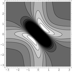
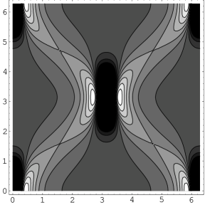
Figure 2: Left: The potential $V(\vartheta_{1},\vartheta_{2})$ as given by (3.1). Here we set $\gamma=1$ and use the geometrical parameters $A=5.5$ Å, $r=4.0$ Å. Darker areas correspond to lower potential energy. Right: The intrapair potential $V_{a}(\psi,\chi)$ in terms of $\psi$ and $\chi$ (parameters as above). Note that beside the $2\pi$ periodicity in $\psi$ and in $\chi$, expressed by $V_{a}(\psi,\chi)=V_{a}(\psi+2\pi,\chi)=V_{a}(\psi,\chi+2\pi)$, there is also a periodicity for simultaneous $\pi$ translations in $\psi$ and $\chi$, i.e. $V_{a}(\psi,\chi)=V_{a}(\psi+\pi,\chi+\pi)$; this follows immediately from (1.5).

3.2 Model parameters

Our model depends on several parameters. Some of these – i.e. $A$, $K_{s}$ and $K_{h}$ are common to the standard Yakushevich model, and we will retain the values given in sect.1 for these.

Note that now $r$ is no longer coinciding with $A$; as the length of H bonds is $\ell_{0}\simeq 3{\rm\AA}$ and $2r=2A-\ell_{0}$, we take $r=4.0{\rm\AA}$; that is, we choose

$$r=4.0{\rm\AA}\ ,\ \ell_{0}=3.0{\rm\AA}\ ,\ A=5.5{\rm\AA}\ ;\ \ \ \lambda=(r/A)\ \simeq\ 0.7272...\ .$$

In order to select a value for $\gamma$, we note that the equilibrium corresponds to $\vartheta_{1}=0=\vartheta_{2}$, while the “maximally open” state of the base pair is obtained for $\vartheta_{1}=\pi=\vartheta_{2}$. Thus $V(\pi,\pi)-V(0,0)$ should be of the order of the energy $\Delta E$ needed to break the base pair; with the choice already accepted for the standard Yakushevich model, we should thus have $V(\pi,\pi)-V(0,0)=\Delta E\simeq 0.1{\rm eV}$.

On the other hand, (3.1) yields

$$V(0,0)\ =\ c_{0}\ -\ \gamma/(A-r)^{3}\ ,\ \ V(\pi,\pi)\ =\ c_{0}\ -\ \gamma/(A+r)^{3}\ ;$$

hence

$$V(\pi,\pi)-V(0,0)=\gamma\left({1\over(A-r)^{3}}-{1\over(A+r)^{3}}\right)={\gamma\over A^{3}}\left({1\over(1-\lambda)^{3}}-{1\over(1+\lambda)^{3}}\right)\ ;$$

thus $\gamma$ should be chosen according to

$$\gamma\ =\ (\Delta E)\ {(A^{2}-r^{2})^{3}\over 2r(3A^{2}+r^{2})}\ =\ (\Delta E)\ A^{3}\ {(1-\lambda^{2})^{3}\over 2\lambda(3+\lambda)}.$$

The relevant parameter for $V$ is $\gamma/4A^{3}$, and by (3.9) we have

$${\gamma\over 4A^{3}}\ =\ {(1-\lambda^{2})^{3}\over 8\lambda(3+\lambda)}\ (\Delta E)\ .$$

With the values given above for $\Delta E$, $A$ and $r$, this yields

$$\gamma\approx 0.34\,{\rm\AA^{3}\,eV}\ ;\ \ \ {\gamma\over 4A^{3}}\ \approx\ 5.1\cdot 10^{-4}\ {\rm eV}\ .$$

3.3 Special soliton solutions

As discussed in sect.2, soliton solutions are obtained as motions in the effective potential $W(\varphi,\eta)$, see (2.14); in the present case $W$ is given – as follows from (2.15) – by

$$\begin{array}[]{rl}W(\varphi,\eta)\ =&-\,c_{0}/(2|\mu|)\ +\\ &+\ [\gamma/(2|\mu|A^{3})]\,\left[7\lambda^{2}+12\cos(2\psi)+4(1+2\lambda^{2})\cos(2\chi)+\right.\\ &\left.+\lambda^{2}\cos(4\chi)-16\lambda\cos\psi\cos\chi\left(1+\cos^{2}\chi\right)\right]\times\\ &\times\left[16\,\left(1+\lambda^{2}\cos^{2}\chi-2\lambda\cos\psi\cos\chi\right)^{5/2}\right]^{-1}\ .\end{array}$$

It is convenient, for the computations to follow, to set $c_{0}$ as given in (3.5).

Figure 3: On the left: The potential $V_{a}(\psi,\chi)$ as a function of $\psi$ for $\chi=0$ (solid line) and as a function of $\chi$ for $\psi=0$ (dashed line); we have used the values $A=5.5$ Å, $r=4$ Åand set $\mu=-1$. On the right: The effective potentials $\widehat{P}(\varphi)=W(\varphi,0)$ (solid) and $\widehat{Q}(\eta)=W(0,\eta)$ (dashed) entering in the determination of the (1,0) and the (0,1) solitons. The additive constant $c_{0}$ has been chosen here so to have $V(0,0)=0$, and energy is measured in units such that $V(\pi,\pi)-V(0,0)=\Delta E=1$.

3.3.1 The (1,0) soliton

The (1,0) soliton is obtained, as discussed in sect.2, by considering $P(\varphi):=V(\varphi,\varphi)$ and solving (2.24). In the present case it results

$$P(\varphi)\ =\ {\gamma\over 4A^{3}}\ \left[{4\over(1-\lambda)^{3}}\ -\ {1+3\cos(2\varphi)-8\lambda\cos(\varphi)+4\lambda^{2}\over(1-2\lambda\cos\varphi+\lambda^{2})^{5/2}}\right]\ ,$$

where we have also used (3.5); we have then to solve

We were not able to perform the integration (2.24) analytically. On the other hand the equivalent equation

$${{\rm d}\varphi\over{\rm d}z}\ =\ \tau\ \sqrt{P(\varphi)}\ ,$$

can be integrated numerically. The result of this integration is shown in fig.4a, where it is also compared with the standard Yakushevich (1,0) soliton.

3.3.2 The (0,1) soliton

The (0,1) soliton is obtained, as discussed in sect.2, by considering $Q(\eta):=V(\eta,-\eta)$ and solving (2.31). In the present case it results

$$Q(\eta)\ =\ {\gamma\over 4A^{3}}\ \left[{4\over(1-\lambda)^{3}}\ -\ {2(1+\cos^{2}\eta)\over(1-2\lambda\cos\eta+\lambda^{2})^{5/2}}\right]\ ,$$

where we have also used (3.5). Again we were not able to perform the integration (2.31) analytically, but the equivalent equation

$${{\rm d}\eta\over{\rm d}z}\ =\ \tau\ \sqrt{Q(\eta)}$$

can be integrated numerically. The result of this integration is shown in fig.4b, where it is also compared with the standard Yakushevich (0,1) soliton.

Figure 4: Comparison of the (1,0) (left) and the (0,1) (right) solitons for the standard Yakushevich model (dotted) and our modified model (solid lines). Despite a certain difference in shape, the size of the (1,0) soliton – corresponding to symmetric motions in the two helices – is remarkably similar in the two models.

4 Improving the intrapair potential II.
Morse potential

The problem of modelling intrapair interactions mediated by H bonds has been tackled in all attempts to provide dynamical models of DNA; among these, the Peyrard-Bishop model (and later improvements by Dauxois [5] and by Barbi, Cocco and Peyrard [1, 2]) has a special relevance in view of its success in describing DNA denaturation [18]. In this, intrapair interactions are described by means of a Morse potential

$$V(r)\ =\ \alpha\ \left[\left(e^{-k(r-r_{0})}-1\right)^{2}-1\right]$$

where $r$ is the distance between (reference atoms belonging to) bases in the given pair.

Note that $V$ has a minimum at $r=r_{0}$ with $V(r_{0})=-\alpha$ and $\lim_{r\to\infty}V(r)=0$, so that $\alpha$ represents the binding energy. We also have $V^{\prime\prime}(r_{0})=2\alpha k^{2}$.

Figure 5: Left: The Morse-PB potential (4.1); here $D=1$, $k=1$ $x_{0}=1$, and we add a constant so that $V(x_{0})=0$. Right: the resulting potential in terms of the rotation angle $\vartheta$, for $\vartheta_{1}=\vartheta_{2}$ (solid) and for $\vartheta_{1}=-\vartheta_{2}$ (dashed).

Thus, albeit the Peyrard-Bishop (PB) model aims at describing a different process undergone by DNA, it is quite natural to consider their modelization of the intrapair potential.

It should be noted that – as pointed out in (4.1) – the Morse-PB potential depends only on the distance between H-bonded atoms, and not on their alignement. This is no surprise, since in the PB model and later improvements the bases lie on a straight line passing through the axis of the double helix.

In our case we have to consider rotational motions, and thus the latter conditions is not holding any more. This raises the question of modelling angular dependence of H bonds in this context; in this section we will consider the isotropic Morse-PB potential (4.1), while in the next section we introduce an angular dependence.

Also, for our purposes it is more convenient to set additive constants in $V$ so that $V(0,0)=0$. Doing this, and denoting as in previous section the distance between (relevant atoms in) the two bases of the pair as $\ell$, and the distance equilibrium as $\ell_{0}$, the Morse-PB potential reads

$$V(\vartheta_{1},\vartheta_{2})\ =\ \alpha\ \left(e^{-k(\ell(\vartheta_{1},\vartheta_{2})-\ell_{0})}-1\right)^{2}\ .$$

Here we have pointed out explicitly the dependence on the angles $\vartheta_{i}$. We also write, for ease of notation,

$$\rho(\vartheta_{1},\vartheta_{2})\ :=\ \ell(\vartheta_{1},\vartheta_{2})\,-\,\ell_{0}\ ,$$

so that (4.2) reads

$$V(\vartheta_{1},\vartheta_{2})\ =\ \alpha\ \left(e^{-k\rho(\vartheta_{1},\vartheta_{2})}-1\right)^{2}\ .$$

4.1 Soliton solutions

With our choice of variables, the distance $\ell$ is written as

$$\ell\ =\ 2A\left[1-\lambda(\cos\vartheta_{1}+\cos\vartheta_{2})+(\lambda^{2}/2)\left(1+\cos(\vartheta_{1}-\vartheta_{2})\right)\right]^{1/2}$$

and of course $\ell_{0}=2A(1-\lambda)$.

By standard computation,

$$\begin{array}[]{l}\rho(\varphi,\varphi)\ =\ 2\,A\ \left(\sqrt{1-2\lambda\cos\varphi+\lambda^{2}}\,-\,(1-\lambda)\right)\ ,\\ \rho(\eta,-\eta)\ =\ 2\,A\ \left(\sqrt{1-2\lambda\cos\eta+\lambda^{2}\cos^{2}\eta}\,-\,(1-\lambda)\right)\ .\end{array}$$

This and (4.4) immediately provide the symmetric and antisymmetric reductions, $P(\varphi)$ and $Q(\eta)$, of the intrapair potential which determine the (1,0) and (0,1) solitons via (2.34) and (2.35); see (2.10) below.

4.2 Model parameters

The intrapair Morse-PB potential $V_{p}$ and hence the effective potential $W$ depend on the two parameters $\alpha$ and $k$; this is at variance with the Yakushevich potential and the dipole-dipole potential considered in sect.3: they both depend on a single parameter.

We can therefore impose two physical conditions in order to fix these parameters; we will retain the values adopted above for the other parameters.

As pointed out above, $\alpha$ represents the dissociation energy for the Morse interaction, supposed to model the H-bond; hence we should have

$$\alpha\ =\ \Delta E\ \simeq\ 0.1\,{\rm eV}\ .$$

We also pointed out that for $\ell\simeq\ell_{0}$, $V\simeq\alpha k^{2}(\ell-\ell_{0})^{2}$; comparing this with (1.5), we require that

$$2\,\alpha\,k^{2}\ =\ K_{p}\ .$$

Here $K_{p}$ should be chosen as in (1.10), taking into account our choice for $r$. This yields

$$k\ =\ \sqrt{K_{p}/(2\alpha)}\ =\ r^{-1}\,\sqrt{K_{p}r^{2}/(2\Delta E)}\ \simeq\ 0.09\,{\rm\AA}^{-1}\ .$$

4.3 Special soliton solutions

The relevant reduced potentials are now

$$\begin{array}[]{l}P(\varphi)\ =\ V(\varphi,\varphi)\ =\ \alpha\,\left(\exp\left[-2Ak\lambda(\sqrt{1-2\lambda\cos\varphi}-(1-\lambda))\right]-1\right)^{2}\ ;\\ Q(\eta)\ =\ V(\eta,-\eta)\ =\ \alpha\,\left(\exp\left[-2Ak\lambda(1-\cos\eta)\right]\right)^{2}\ .\end{array}$$

The equations (2.34) and (2.35) governing the special (1,0) and (0,1) soliton solutions are again impossible to solve analytically, but can be integrated numerically. The results of these integration are shown in fig.6, where we also plot the standard Yakushevich solitons of the same topological number for comparison. Quite remarkably, again the overall size is about the same as with the standard Yakushevich model.

Figure 6: Special soliton solutions for Morse intrapair potential (solid lines) compared with standard Yakushevich solitons (dotted). Left: the (1,0) soliton; right: the (0,1) soliton. See text for parameters values; we plot solutions for $v=0$.

5 Improving the intrapair potential III.
Morse potential with a directional term

As mentioned in the beginning of the previous section, the Morse-PB potential provides an “isotropic” description of the H-bond mediated intrapair interaction. On the other hand, as discussed in the Introduction, once we allow rotational motions, hence the possibility that the alignment between the atoms intervening in the H-bond is broken, we should consider the directional nature of the H-bonds. This makes that the bases are essentially free (as far as this interaction is concerned) once they are more than a few degrees away from the equilibrium position.

It should be stressed that in our model the bases cannot come any nearer than their equilibrium distance; that is, we do not have to worry about the region on the left of the minimum of $V_{p}(r)$.

A simple way to modify the Morse-PB potential in order to take into account the angular dependence of H-bonds is to introduce a prefactor $A(\vartheta_{1},\vartheta_{2})$ which is unity at equilibrium and goes rather quickly to zero when at least one of the bases rotate away from this. It is convenient to choose a smooth function for this $A$; it should moreover be $2\pi$-periodic in both its argument.

The natural candidate for a prefactor with these features is a gaussian-like function: we choose (no confusion should be possible with the $\gamma$ used in sect.3)

$$A(\vartheta_{1},\vartheta_{2})\ :=\ \exp[-\gamma((1-\cos\vartheta_{1})+(1-\cos\vartheta_{2}))]\ .$$

We thus have a modified Morse-PB potential

$$V\ =\ A(\vartheta_{1},\vartheta_{2})\ \left[\alpha\left((e^{-k\rho(\vartheta_{1},\vartheta_{2})}-1)^{2}-1\right)\right]$$

where we have used notation introduced in sect.4 above. Adding a constant $\alpha$ so that $V(0,0)=0$, the explicit expression for this is

$$V\ =\ \alpha\ \exp[-\gamma(1-\cos\vartheta_{1})(1-\cos\vartheta_{2})]\ \left[\left(1-\exp[-k\rho(\vartheta_{1},\vartheta_{2})]-1\right)^{2}-1\right]+\alpha\ .$$

We will take the same values as in the previous sections for the parameters of the Morse potential. As for the newly introduced parameter $\gamma$, this should be chosen so that the H-bond interaction is conveniently reduced when the relevant atoms are not properly aligned. A natural criterion is to require $A(\theta_{0},\theta_{0})=a_{0}$ with somewhat arbitrary values for $\theta_{0}$ and $a_{0}$. If we choose $\theta_{0}=\pi/4$ and $a_{0}=1/10$, we get

$$\gamma\ \simeq\ 4\ ;$$

this will be our choice. The resulting potential is plotted in fig.7.

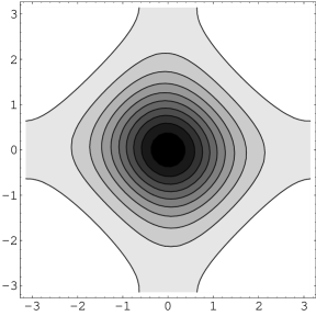
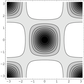
Figure 7: The Morse directional potential $V(\vartheta_{1},\vartheta_{2})$ as given by (5.3) with $\gamma=4$ (left); and the same in adapted coordinates $\psi,\chi$, i.e. $V_{a}(\psi,\chi)=V(\psi+\chi,\psi-\chi)$ (right). These can be compared with fig.2.

Special soliton solutions are obtained as usual by numerically solving equations (2.34) and (2.35). The relevant reduced effective potentials are in this case

$$\begin{array}[]{rl}P(\varphi)\ =&\alpha\left[1\ +\ e^{-2\gamma(1-\cos\varphi)}\,\left((\exp[-2kAF]-1)^{2}\,-\,1\right)\right]\ ,\\ Q(\eta)\ =&\alpha\left[1\ +\ e^{-2\gamma(1-\cos\eta)}\,\left((\exp[-2kAG]-1)^{2}\,-\,1\right)\right]\ ,\end{array}$$

where we have defined, for ease of writing,

$$F\,=\,\sqrt{1-2\lambda\cos\varphi+\lambda^{2}}\,-\,(1-\lambda)\ ,\ G\,=\,\lambda\,(1-\cos\eta)\ .$$

Figure 8: The (1,0) soliton (left) and the (0,1) soliton (right) solutions for the Morse intrapair potential with directional term (5.3) (solid lines) and, for comparison purposes, for the standard Yakushevich model. Here parameters of the Morse potential and geometrical parameters are as in section 4, i.e. $A=5.5$ Å, $r=4.0$ Å, $\lambda=0.73$, $\alpha=0.1$ eV, $k=0.088$ ${\rm\AA}^{-1}$, and $\gamma=4$.

Needless to say, our choice for the parameter $\gamma$ was to a large extent arbitrary; we should then check that the resulting soliton solutions are not strongly dependent on such arbitrary choice. To this purpose, we have integrated the equations also using different values for $\gamma$, and it resulted that the soliton solutions are very little dependent on this. The results of integration with $\gamma=1$ and for $\gamma=10$ are shown, together with the solution obtained for $\gamma=4$, in fig.9.

Figure 9: Dependence of the (1,0) (left) and (0,1) (right) soliton solutions for the Morse intrapair potential with directional term on the value of the parameter $\gamma$. Keeping all other parameters equal (values as in fig.8 above), we plot solutions for $\gamma=4$ (solid line) together with those for $\gamma=1$ (dashed) and for $\gamma=10$ (dotted). Solutions are extremely similar.

6 Discreteness effects

We have described solitons in the continuum approximation; our original model was however a discrete one and as well known, going back to a discretized description the soliton propagation results to be hindered by the Peierls-Nabarro barrier [18].

The intrapair potentials considered in this note lead to effective potentials which are steeper than the one corresponding to the original Yakushevich potential near the equilibrium position, but have a nearly flat region at larger amplitude of the $\theta_{i}$ fields; moreover, they lead to soliton solutions which have a much larger curvature at the interface between the nearly quiescent region and the “transition” region (in which the field passes from 0 to $2\pi$), and a nearly zero curvature in the transition region. These effects lead to opposite variation, and so the net effect should be evaluated quantitatively in order to understand which contribution is larger.

We thus want to evaluate the Peierls barrier for the different potentials we have considered; we will focus on the (1,0) special soliton solutions. The Peierls barrier for a given travelling wave can be evaluated as follows.

First of all, we can just consider static solutions $\phi(z)=\varphi(x)$, i.e. set $v=0$; for these the energy of the configuration will not include the kinetic term, and reduce (see sect.1) to

$$H\ =\ U_{s}\ +U_{p}\ .$$

Note that the balance between these two contribution is only marginally dependent on the model we consider: indeed parameters were determined by the strength of the stacking and the pairing interactions, as they result from experiments.

The field $\varphi(x)$ should now be replaced by the array of values

$$\phi_{n}\ :=\ \varphi(n\delta)\ .$$

The stacking energy $U_{s}$ is given by (1.2). As in our case $\vartheta_{1}(x)=\vartheta_{2}(x)=\varphi(x)$, the latter reads simply

$$U_{s}\ =\ K_{s}\ \sum_{n}\,(\phi_{n+1}-\phi_{n})^{2}\ ;$$

note this holds for any Y-like model, and in particular for all the models we have considered.

The pairing energy $U_{p}$ depends on the intrapair potential $V$, and is given, see again sect.1 and in particular (1.4), by the sum of the pairing energy of all base pairs. In our case,

$$U_{p}\ =\ \sum_{n}\,V(\phi_{n},\phi_{n})\ =\ \sum_{n}\,P(\phi_{n})\ .$$

Using (6.2), we can express the energy for the chain configuration in terms of the soliton field configuration; indeed (6.3) and (6.4) are also written as

$$U_{s}\,=\,K_{s}\,\sum_{n}\,[\varphi((n+1)\delta)-\varphi(n\delta)]^{2}\ ,\ U_{p}\,=\,\sum_{n}\,P[\varphi(n\delta)]\ .$$

We introduce now a shift parameter $s\in[0,1]$, and compute the energy when the configuration is shifted by $s\delta$:

$$H(s)\ :=\ K_{s}\ \sum_{n}\,[\varphi((n+1+s)\delta)-\varphi((n+s)\delta)]^{2}\ +\ \sum_{n}\,P[\varphi((n+s)\delta)]\ .$$

The Peierls barrier is then given by the different between the maximum and the minimum over $s\in[0,1]$ of the function

$$B(s)\ :=\ H(s)-H(0)\ .$$

We have computed this for the different models considered here; the results are summarized in the table below:

Intrapair potential	Peierls barrier
Standard Y	$4.3\cdot 10^{-5}$ eV
Dipole	$2.3\cdot 10^{-2}$ eV
Morse-PB	$3.2\cdot 10^{-7}$ eV
Directional Morse ($\gamma=4$)	$1.1\cdot 10^{-2}$ eV
Directional Morse ($\gamma=1$)	$3.5\cdot 10^{-4}$ eV

It results that considering directional rather than isotropic potentials (that is, dipole-dipole rather than the standard Y potential; or directional Morse rather than isotropic Morse-PB) leads to a higher Peierls barrier, i.e. isotropic potentials make us underestimate its height.

On the other hand, a Morse-type potential (Morse-PB rather than standard Y; or directional Morse rather than dipole-dipole) lead to a lower Peierls barrier.

7 Discussion and conclusions

We have considered the Yakushevich model for DNA torsion dynamics, in a version modified by introducing different expressions for the intrapair potential $V(\vartheta_{1},\vartheta_{2})$; these were:

(a) a dipole-dipole interaction, which takes into account the essentially dipolar nature of the H bonds mediating the intrapair interaction between bases in a pair;

(b) a Morse-type potential, as often used to model H-bonds;

(c) a Morse-type potential modified by introducing a prefactor which takes into account the directional nature of the essentially dipolar interaction at the origin of H-bonds.

We have focused on travelling soliton solutions, in particular the special ones – with topological indices (1,0) and (0,1) respectively – in which only one of the fields $\psi$ and $\chi$ varies from the equilibrium configuration.

We found that these solutions vary quite little when we consider these different expressions for the potential (on the other hand, the Peierls barrier is quite different in the different cases considered). In particular, the width of the soliton is, provided we choose parameters appearing in the model following the same physical criteria, of the same order of magnitude.

This should not be too surprising: after all, once we fix boundary conditions – i.e. the topological indices – the solution results from a balance between the stacking interaction (which would favor very smooth transitions from one vacuum to the other) and the on-site intrapair potential (which would favor as little bases as possible being away from minima of this potential). Thus, the width of the soliton depends essentially on the ration between strength of these two interactions.

The Yakushevich model is concerned with DNA torsion dynamics; according to the pioneering proposal of Englander et al. [8], topological (kink) solitons in this dynamics should somehow correspond to the “transcription bubbles” which are formed when RNA-Polymerase binds to the DNA double chain; from this point of view, the main success of the Yakushevich model was to provide the correct size for these nonlinear excitations.

We found that the soliton solutions have a different shape in the standard and in the modified Yakushevich models; but their size is not very different in the different models. We have also computed the Peierls barrier for the different models, finding a quite large range of variability.

In conclusion, our study suggests that:

• (A) The standard Yakushevich model captures to a large extent the essential part of DNA dynamics as it can be described by simple models with a single degree of freedom per nucleotide.

• (B) On the other hand, study of the standard Yakushevich model can have led to an overestimation of the Peierls-Nabarro barrier to be overcome by the topological solitons to move along the discrete DNA double chain.

Point (B) suggests that solitons with too low speed could actually be unable to propagate along the chain, and thus set also a minimum speed – and not just a maximum one, see sect.2 – for such solutions, at variance with the analysis of purely continuous solitonic excitations in the Yakushevich model [11].

Point (A) shows that it is pointless to attempt an improvement of the standard Yakushevich model – e.g. to reconcile the predictions of the model with different physical requirements, which leads to contrasting tuning of the parameter values [26] – simply by improving the expressions of the intrapair (pairing) potential.

Albeit we have not considered this point here, the results of this study and the qualitative discussion above seem to suggest that the same applies to some extent for improved expressions of the stacking potential. In this respect we recall, however, that recent work by Saccomandi and Sgura [20] points out new phenomena appearing as a nonlinear stacking potential is considered.

Thus the main result of our investigation is that in order to go over the limitation of the standard Yakushevich model we should not try to investigate more and more detailed description of the interactions between different parts of the DNA molecule within the description provided by the standard Yakushevich model, but rather consider a more detailed model, maybe with equally rough approximation of the interactions. In the language of [24], we should go to a higher level in the hierarchy of DNA models.

This will be done in a different note [3], where a Y-type model with more degrees of freedom will be considered. On the other hand, the investigation reported in the present paper suggests that the new model can be tackled, in the first approximation, considering very simple expressions for interaction potentials.

References

- [1] M. Barbi, S. Cocco and M. Peyrard, “Helicoidal model for DNA opening”, Phys. Lett. A 253 (1999), 358-369
- [2] M. Barbi, S. Cocco, M. Peyrard and S. Ruffo, “A twist-opening model of DNA”, J. Biol. Phys. 24 (1999), 97-114
- [3] M. Cadoni, R. De Leo and G. Gaeta, “A composite Y model of DNA torsion dynamics”; forthcoming paper
- [4] C. Calladine and H. Drew, Understanding DNA, Academic Press (London) 1992; C. Calladine, H. Drew, B. Luisi and A. Travers, Understanding DNA ( edition), Academic Press (London) 2004
- [5] Th. Dauxois, “Dynamics of breather modes in a nonlinear helicoidal model of DNA”, Phys. Lett. A 159 (1991), 390-395
- [6] A.S. Davydov, Solitons in Molecular Systems, Kluwer (Dordrecht) 1981
- [7] A. Dubrovin, S.P. Novikov and A. Fomenko, Modern geometry, Springer (Berlin) 1984
- [8] S.W. Englander, N.R. Kallenbach, A.J. Heeger, J.A. Krumhansl and A. Litwin, “Nature of the open state in long polynucleotide double helices: possibility of soliton excitations”, PNAS USA 77 (1980), 7222-7226
- [9] G. Gaeta, “On a model of DNA torsion dynamics”, Phys. Lett. A 143 (1990), 227-232
- [10] G. Gaeta, “Solitons in planar and helicoidal Yakushevich model of DNA dynamics”, Phys. Lett. A 168 (1992), 383-389
- [11] G. Gaeta: “A realistic version of the Y model for DNA dynamics; and selection of soliton speed”; Phys. Lett. A 190 (1994), 301-308
- [12] G. Gaeta, “Results and limits of the soliton theory of DNA transcription”, J. Biol. Phys. 24 (1999), 81-96
- [13] G. Gaeta, “Solitons in the Yakushevich model of DNA beyond the contact approximation”, preprint 2006
- [14] G. Gaeta, C. Reiss, M. Peyrard and Th. Dauxois, “Simple models of non-linear DNA dynamics”, Rivista del Nuovo Cimento 17 (1994) n.4, 1–48
- [15] J.A. Gonzalez and M. Martin-Landrove, “Solitons in a nonlinear DNA model”, Phys. Lett. A 191 (1994), 409-415
- [16] R. Lavery, A. Lebrun, J.F. Allemand, D. Bensimon and V. Croquette, “Structure and mechanics of single biomolecules: experiments and simulation”, J. Phys.: Condens. Matter 14 (2002), R383-R414
- [17] M. Peyrard (editor), Nonlinear excitations in biomolecules, (Proceedings of a workshop held in Les Houches, 1994), Springer (Berlin) and Les Editions de Physique (Paris) 1995
- [18] M. Peyrard, “Nonlinear dynamics and statistical physics of DNA”, Nonlinearity 17 (2004) R1-R40
- [19] M. Peyrard and A.R. Bishop, “Statistical mechanics of a nonlinear model for DNA denaturation”, Phys. Rev. Lett. 62 (1989), 2755-2758
- [20] G. Saccomandi and I. Sgura, “The relevance of nonlinear stacking interactions in simple models of double-stranded DNA”, preprint 2006
- [21] W. Saenger, Principles of nucleic acid structure, Springer (Berlin) 1984
- [22] S.B. Smith, L. Finzi and C. Bustamante, “Direct mechanical measurements of the elasticity of single DNA molecules by using magnetic beads”, Science 258 (1992), 1122-1126
- [23] L.V. Yakushevich, “Nonlinear DNA dynamics: a new model”, Phys. Lett. A 136 (1989), 413-417
- [24] L.V. Yakushevich, “Nonlinear DNA dynamics: hyerarchy of the models”, Physica D 79 (1994), 77-86
- [25] L.V. Yakushevich, Nonlinear Physics of DNA, Wiley (Chichester) 1998; second edition 2004
- [26] L.V. Yakushevich, A.V. Savin and L.I. Manevitch, “Nonlinear dynamics of topological solitons in DNA”, Phys. Rev. E 66 (2002), 016614