Solitons in the Yakushevich model of DNA beyond the contact approximation

Abstract

The Yakushevich model of DNA torsion dynamics supports soliton solutions, which are supposed to be of special interest for DNA transcription. In the discussion of the model, one usually adopts the approximation $\ell_{0}\to 0$, where $\ell_{0}$ is a parameter related to the equilibrium distance between bases in a Watson-Crick pair. Here we analyze the Yakushevich model without $\ell_{0}\to 0$. The model still supports soliton solutions indexed by two winding numbers $(n,m)$; we discuss in detail the fundamental solitons, corresponding to winding numbers (1,0) and (0,1) respectively.

Introduction

Following the pioneering paper and proposal by Englander, Kallenbach, Heeger, Krumhansl and Litwin Eng , a number of authors considered simple idealized models for the roto/torsional dynamics of DNA one, with the aim of describing nonlinear solitonic excitations which – according to the ideas of Englander et al. – would be related to the transcription bubble which travels along with RNA-Polymerase in the DNA transcription process, and would thus play a functional role in this process.

These models are based on modelling the DNA molecule as a double chain of coupled pendulums; the relevant nonlinear excitations would then be (topological and dynamical) solitons like those of the sine-Gordon equation. For a review of the approaches in this direction, see YakuBook ; for general properties of DNA and its functions, see e.g. CD .

It should be noted that in a related approach – but in a different direction – the stretching motions of the DNA molecule (related to DNA denaturation) have also been studied by nonlinear models, see in particular the Peyrard-Bishop model PB and extensions thereof BCP ; BCPR ; PeyNLN . In this note we will focus on roto/torsional dynamics, and thus we will not deal with Peyrard-Bishop like models.

Coming back to rotational dynamics, a very interesting and quite successful model (also called Y-model) was put forward by prof. L.V. Yakushevich YakPLA . See YakPhD ; YakuBook ; YakPRE for further results and extensions.

In the Yakushevich model, the DNA molecule is considered homogeneous (i.e. all nucleotides are considered as identical), and the state of each nucleotide is described by a single degree of freedom; in fact, a rotation angle of the base belonging to the nucleotide around the $C_{1}$ atom in the sugar-phosphate backbone. Each nucleotide (or base) is represented as a disk.

Interaction between successive nucleotides on each DNA helix is via a harmonic potential, while the intrapair interaction (i.e. interaction between bases in a Watson-Crick pair, and through these between the corresponding nucleotides) is modelled by a potential which albeit harmonic in the distance, becomes anharmonic when described in terms of the relevant degrees of freedom, i.e. rotation angles. More precisely, with $\ell$ the distance between relevant points $B_{1}$ and $B_{2}$ (see fig.2) of the disks representing nucleotides in the Yakushevich model, and $\ell_{0}$ the distance between the points $B_{1}$ and $B_{2}$ in the equilibrium (i.e. the B-DNA) configuration, the intrapair potential is $V_{0}=(1/2)K_{p}(\ell-\ell_{0})^{2}$, with $K_{p}$ a dimensional constant.

In the standard Yakushevich model, one considers the approximation $\ell_{0}=0$, which leads to a number of computational simplification; we call this the contact approximation, as it corresponds to having contact between the disks representing nucleotides at same site on the two chains. However, as pointed out by Gonzalez and Martin-Landrove GML , $\ell_{0}=0$ is a singular case in that the description one thus obtains is not structurally stable: as soon as we consider $\ell_{0}\not=0$, certain qualitative features of the model dynamics are changed.

In this note we will analyze the Yakushevich model beyond the contact approximation, i.e. with a nonzero value for the parameter $\ell_{0}$; we focus in particular on travelling wave solutions and soliton-like excitations, as they are the most important objects in the approach of Englander et al. Eng .

It turns out that in this case soliton solutions are still present, albeit the simple form obtained with the contact approximation is replaced by an expression involving elliptic integrals. The qualitative form of soliton solutions is little changed with respect to the standard Y-model; as for their width, it is very moderately increased (see fig.5), still remaining in the same order of magnitude.

Acknowledgements. I would like to thank M. Cadoni and R. De Leo for useful discussions, and anonymous referees for constructive criticisms. This work received support by the Italian MIUR (Ministero dell’Istruzione, Università e Ricerca) under the program COFIN2004, as part of the PRIN project “Mathematical Models for DNA Dynamics ($M^{2}\times D^{2}$)”.

I The model

In the Yakushevich model the DNA double chain is considered to be infinite, and all bases are considered as having the same physical characteristics; it is thus an “ideal” DNA model according to Yakushevich’s classification YakPhD ; YakuBook .

Moreover, each nucleotide is considered as a single unit and its state described in terms of an angular variable. More precisely, each nucleotide is modelled as a rigid disk which can rotate around an axis and has a moment of inertia $I$ around this axis, see fig.1. The rotation of the nucleotide at site $i\in{\bf Z}$ on the chain $a$ ($a=1,2$) is described by an angle $\vartheta^{(a)}_{i}$; we orient all angles in counterclockwise direction. When we are referring to a specific base pair, we write simply $\vartheta_{1},\vartheta_{2}$ for $\vartheta^{(1)}_{i},\vartheta^{(2)}_{i}$.

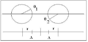
Figure 1: Left: A base pair in the Yakushevich model. The only moving elements in nucleotides are the bases; these are represented as identical disks of radius $r$, which can rotate around their centers. The disks centers lie at a distance $A$ from the double helix axis, and the rotation angles (positive in counterclockwise direction) are $\theta_{1}$, $\theta_{2}$ respectively. The distances $A$ and $r$ are related via $A=r+\ell_{0}/2$, and $\ell_{0}$ is the distance between the disks, $\ell_{0}=2(A-r)$. Right: disks represent bases and are located on the double helix; two disks as those marked in black interact via the helicoidal terms considered in the appendix.

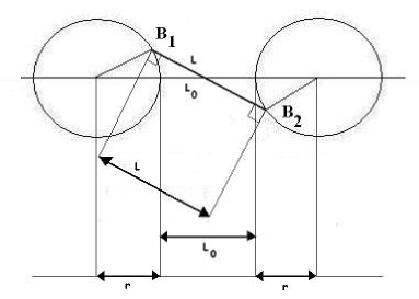
Figure 2: Further detail of the base pair modelling in the Yakushevich model, showing in particular the points $B_{1}$ and $B_{2}$ whose spatial distance is $\ell$. For graphics convenience, $\ell$ and $\ell_{0}$ have been denoted as $L$ and $L_{0}$ in this plot.

The model is described by a Lagrangian $L=T-U$. The kinetic energy is

$$T\ =\ \sum_{a}\,\sum_{i}{I\over 2}\,({\dot{\vartheta}}^{(a)}_{i})^{2}\ .$$

The potential energy $U$ is the sum of two terms; these are the stacking ($U_{s}$) term and the pairing one $(U_{p}$). Thus $U\,=\,U_{s}+U_{p}$. (There is a third term $U_{h}$ if we consider the so-called “helicoidal” version of the model Dauhel ; Gaehel ; introducing $U_{h}$ leads to qualitative changes in the small amplitude regime. However, the additional term $U_{h}$ is not relevant to fully nonlinear dynamics, and thus we will not consider it. See the appendix for small amplitude dynamics, where it matters to introduce this term.)

The first term corresponds to a harmonic potentials (the choice of harmonic potentials for these term is common to nearly all DNA models PeyNLN ; YakuBook ) and depend on a dimensional coupling constant $K_{s}$. It describes backbone torsion and stacking interactions between bases at nearby sites on the same chain; in our notation it is given by

$$U_{s}\ =\ {K_{s}\over 2}\ \sum_{a}\,\sum_{i}\,\left(\vartheta^{(a)}_{i+1}-\vartheta^{(a)}_{i}\right)^{2}\ .$$

As for the $U_{p}$ (pairing) term, it describes the nonlinear interactions between bases in a pair, i.e.

$$U_{p}\ =\ \sum_{i}\ V_{0}(\vartheta^{(1)}_{i},\vartheta^{(2)}_{i})\ .$$

The potential $V_{0}$ is not harmonic in terms of the angles $\vartheta^{(a)}_{i}$: here lies the nonlinearity of the dynamics and hence the hearth of the Yakushevich model. It is assumed that

$$V_{0}\ =\ (1/2)\,K_{p}(\ell-\ell_{0})^{2}\ ,$$

where $\ell$ is the distance between the atoms which are bridged by the H bonds – these are represented in the model by reference points on the border of the disk representing the bases, and more precisely by the point which lies nearer to the double helix axis for $\vartheta=0$ – and $\ell_{0}$ is this distance in the equilibrium configuration described by $\vartheta^{(a)}_{i}=0$. We also write $r+\ell_{0}/2=A$ for the distance between the center of the disks representing nucleotides and the axis of the double helix.

This harmonic potential becomes anharmonic in terms of the angles $\vartheta^{(a)}_{i}$. Indeed, with simple algebra (and writing $\vartheta_{a}$ for $\vartheta^{(a)}_{i}$) we have

$$\begin{array}[]{rl}\ell^{2}=&(\ell_{0}^{2}+4\ell_{0}r+6r^{2})-2r(\ell_{0}+2r)[\cos\vartheta_{1}+\cos\vartheta_{2}]+\\ &+2r^{2}\,\cos(\vartheta_{1}-\vartheta_{2})\ .\end{array}$$

In the standard Yakushevich model, one considers the contact approximation $\ell_{0}=0$, which entails $A=r$; with this, and omitting a constant term which plays no role, $U_{p}=K_{p}r^{2}\sum_{i}[\cos(\vartheta^{(1)}_{i}-\vartheta^{(2)}_{i})-2(\cos\vartheta^{(1)}_{i}+\cos\vartheta^{(2)}_{i})]$. We refer e.g. to GRPD ; YakuBook for further detail on the standard Yakushevich model.

In this note we will not adopt the contact approximation $\ell_{0}\to 0$, and instead consider the potential energy (1.3) with $V_{0}$ given by (1.4), (1.5).

Let us provide an explicit expression for $V_{0}(\vartheta_{1},\vartheta_{2})$. With the notation introduced above, $\ell^{2}=(2A-r\cos\vartheta_{1}-r\cos\vartheta_{2})^{2}+(r\sin\vartheta_{1}+r\sin\vartheta_{2})^{2}$. Introducing the adimensional parameter $\lambda=r/A$, this yields

$$\begin{array}[]{rl}V_{0}=&(1/2)K_{p}(\ell-\ell_{0})^{2}\\ =&2\,K_{p}\,A^{2}\,\left[(1-\lambda)-\sqrt{\rho(\vartheta_{1},\vartheta_{2})}\right]^{2}\ ,\end{array}$$

where we have written for short

$$\begin{array}[]{rl}\rho(\vartheta_{1},\vartheta_{2})\ :=&\ \left(1-\lambda(\cos\vartheta_{1}+\cos\vartheta_{2})+\right.\\ &\left.+(\lambda^{2}/2)[1+\cos(\vartheta_{1}-\vartheta_{2})]\right)\ .\end{array}$$

Needless to say, $V_{0}(\vartheta_{1},\vartheta_{2})\geq 0$ for all values of $\vartheta_{1},\vartheta_{2}$, the equality being satisfied only for the equilibrium position $\vartheta_{1}=\vartheta_{2}=0$.

It should be stressed that this minimum of $V_{0}$ is non-quadratic, as remarked by GML ; indeed, expanding around the equilibrium $\vartheta_{1}=\vartheta_{2}=0$, we get

$$\begin{array}[]{l}V_{0}(\varepsilon\vartheta_{1},\varepsilon\vartheta_{2})\ =\ (K_{p}/2)\,\left(r[r(\vartheta_{1}-\vartheta_{2})^{2}+\right.\\ \left.\ -2A(\vartheta_{1}^{2}+\vartheta_{2}^{2})]\,/\,[4(A-r)]\right)^{2}\ \varepsilon^{4}\ +\ O(\varepsilon^{6})\ .\end{array}$$

The equations of motion – i.e. the Euler-Lagrange equations arising from the modified Lagrangian – are

$$\begin{array}[]{rl}I{\ddot{\vartheta}}^{(a)}_{n}=&K_{s}\left(\vartheta^{(a)}_{n+1}-2\vartheta^{(a)}_{n}+\vartheta^{(a)}_{n-1}\right)+\\ &-\partial V_{0}(\vartheta^{(1)}_{n},\vartheta^{(2)}_{n})/\partial\vartheta^{(a)}_{n}\ .\end{array}$$

It is convenient, as in the standard Yakushevich model, to pass to variables

$$\psi_{n}={\vartheta^{(1)}_{n}+\vartheta^{(2)}_{n}\over 2}\ ,\ \chi_{n}={\vartheta^{(1)}_{n}-\vartheta^{(2)}_{n}\over 2}\ ;$$

these correspond to $\vartheta^{(1)}_{n}=\psi_{n}+\chi_{n}$ and $\vartheta^{(2)}_{n}=\psi_{n}-\chi_{n}$.

In terms of the $\psi,\chi$ variables the eqs. (1.8) read

$$\begin{array}[]{rl}I{\ddot{\psi}}_{n}=&K_{s}\left(\psi_{n+1}-2\psi_{n}+\psi_{n-1}\right)\,-\,(1/2)\left(\partial V/\partial\psi\right)\ ,\\ I{\ddot{\chi}}_{n}=&K_{s}\left(\chi_{n+1}-2\chi_{n}+\chi_{n-1}\right)\,-\,(1/2)\left(\partial V/\partial\chi\right)\ .\end{array}$$

Here we have denoted by $V=V(\psi,\chi)$ the expression of $V_{0}(\vartheta_{1},\vartheta_{2})$ in terms of the new variables; that is,

$$V(\psi,\chi)\ :=\ V_{0}(\psi+\chi,\psi-\chi)\ .$$

II Physical values of the parameters

Several dimensional parameters appear in our model Lagrangian and hence in the Euler-Lagrange equations of motion. We will discuss the model and its predictions for generic values, but specific values apply to the DNA molecule; for the geometric ones we will refer for definiteness to B-DNA.

The parameter $A$ represents the distance from the center of rotation of the disks representing nucleotides to the axis of the double helix. Taking this center at the $C_{1}$ atoms (as in the derivation of parameters in the standard Yakushevich model), we get $2A=11.1$Åfor AT pairs and $2A=10.8$Åfor GC pairs Vol . We will take the intermediate value $A=5.48$Å. (Had we taken the center of rotation on the phosphodiester chain, $A\simeq 10$Åwould have resulted YakuBook ).

The choice of the $C_{1}$ atom as center of rotation for the nucleotides is not only conformal to discussion of the standard Yakushevich model GaeJBP ; GRPD ; YakuBook , but also physically sound: indeed the phosphodiester chain in the backbone is a very flexible polymer (as also confirmed by the success of Poland-Scheraga type models based on such flexibility BLPT ; KMP ), while the complex formed by the sugar ring and the attached base can be seen in a first approximation as a rigid body ZC .

As for $r$ and $\ell_{0}$, these satisfy $2A=2r+\ell_{0}$; thus $r$ is obtained as $r=A-\ell_{0}/2$. Here $\ell_{0}$ is the length of the H bond bridging bases in a pair, while $r$ is the radius of disks representing bases. The physical meaning of $r$ would be the distance from the center of rotation for disks (the $C_{1}$ atom in the sugar ring) to the atoms bridged by the intrapair H bonds.

This distance is quite different from one base to the other, and also different for different H-bonded atoms in the same base. Thus we prefer to set the parameter of our idealized model in terms on the much more uniform value of $\ell_{0}$, which is $\ell_{0}\simeq 2.9\pm 0.1$Åfor the different H bonds in Watson-Crick pairs (see sect.7.2 of Vol ). We will adopt the value $\ell_{0}=2.9$Å. With these choices, $r\simeq 4.0$Å, and hence $\lambda=r/A=[1-\ell_{0}/(2A)]=0.74\simeq 3/4$.

Finally, $\delta$ represents the interbase distance along the double helix axis; in B-DNA this is $\delta=3.4$Å.

After discussing the geometrical parameters, let us now come to the dynamical ones. First of all, we have the moment of inertia $I$; this is rather different for different bases (detailed values are given e.g. in ZC ). Taking an average over different values, we will adopt as in GaeJBP the value $I=3\cdot 10^{-37}\,{\rm cm}^{2}\,{\rm g}$. As for the coupling constants $K_{s}$ and $K_{p}r^{2}$ (and $K_{h}$ considered in the appendix), we will also adopt the values given in GaeJBP , i.e. $K_{s}=0.13$eV, $K_{p}r^{2}=0.025$eV, $K_{h}=0.009$eV.

In our discussion of soliton solutions and their width, we used the parameters $\mu$ and $B$; the first of these depends on the speed of the soliton, which is a free parameter (provide it is smaller than the limiting value $\sqrt{K_{s}/I}\delta$, see sect.3) in the Yakushevich model. For $v=0$, we get $\mu=-K_{s}\delta^{2}$. The parameter $B^{-1}=b\delta$ is defined in terms of $\mu$ by (5.8) below. With our choices for the dimensional parameters, and $\mu$ as above, we get $b\simeq(3/8)2.28\simeq 0.86$, and hence $B^{-1}\simeq 0.86\delta$, $B\simeq 0.34\AA^{-1}$.

III Continuum approximation

In discussing (1.10), it is convenient to promote the arrays $\{\psi_{n}(t)\}$ and $\{\chi_{n}(t)\}$ ($n\in{\bf Z}$) to fields $\psi(x,t)$ and $\chi(x,t)$ (no confusion should be possible between old dependent variables and fields), the correspondence being given by

$$\psi_{n}(t)\ \simeq\ \psi(n\delta,t)\ ,\ \ \chi_{n}(t)\ \simeq\ \chi(n\delta,t)\ .$$

Here $\delta$ is the spacing between successive sites of each chain; in B-DNA we have $\delta=3.4$Å. (It is of course also possible to pass to adimensional units in the spatial variable, i.e. set $\xi=x/\delta$, and consider $\psi(\xi,t)$, $\chi(\xi,t)$ so that e.g. $\psi_{n}(t)=\psi(\xi,t)$ for $\xi=n$.)

With this, (1.10) reads

$$\begin{array}[]{rl}I\psi_{tt}(x,t)=&K_{s}\left(\psi(x+\delta,t)-2\psi(x,t)+\psi(x-\delta,t)\right)+\\ &\ -\ (1/2)\left(\partial V/\partial\psi\right)(x,t)\ ,\\ I\chi_{tt}(x,t)=&K_{s}\left(\chi(x+\delta,t)-2\chi(x,t)+\chi(x-\delta,t)\right)+\\ &\ -\ (1/2)\left(\partial V/\partial\chi\right)(x,t)\ .\end{array}$$

If now we assume that $\psi(x,t)$ and $\chi(x,t)$ vary slowly in space compared with the length scale set by lattice spacing, we can write

$$\begin{array}[]{l}\psi(x\pm\delta,t)=\psi(x,t)\pm\delta\psi_{x}(x,t)+(\delta^{2}/2)\psi_{xx}(x,t)\ ,\\ \chi(x\pm\delta,t)=\chi(x,t)\pm\delta\chi_{x}(x,t)+(\delta^{2}/2)\chi_{xx}(x,t)\ .\end{array}$$

Inserting these into (3.2), we obtain the equations of motion for the Yakushevich model in the continuum approximation:

$$\begin{array}[]{rl}I\psi_{tt}(x,t)=&K_{s}\delta^{2}\psi_{xx}(x,t)-(1/2)\left(\partial V/\partial\psi\right)(x,t)\ ,\\ I\chi_{tt}(x,t)=&K_{s}\delta^{2}\chi_{xx}(x,t)-(1/2)\left(\partial V/\partial\chi\right)(x,t)\ .\end{array}$$

We omit from now on to specify at which point functions should be evaluated, as we got a local formulation. We will also consider, where appropriate, $\vartheta_{1}$ and $\vartheta_{2}$ as fields.

The PDEs (3.4) should be supplemented with a side condition specifying the function space to which acceptable solutions belong. The physically natural condition is that of finite energy; that is, we should require that the integral

$$\int_{-\infty}^{+\infty}\left[{1\over 2}\left(I(\psi_{t}^{2}+\chi_{t}^{2})+K_{s}(\psi_{x}^{2}+\chi_{x}^{2})\right)+{1\over 2}V(\psi,\chi)\right]{\rm d}x$$

is finite; if this condition is satisfied at $t=0$, it will be so for any $t$.

It should be mentioned that the Yakushevich equations (3.4) correspond, in the $\ell_{0}=0$ approximation, to classical ones when only one field is nonzero: indeed for $\chi=0$ they reduce to the sine-Gordon equation, while for $\psi=0$ one gets the so-called ”double sine-Gordon” equation, which appears in many physical contexts BCG ; CDeg .

IV Travelling wave solutions

Next we focus on travelling wave solution for (3.4). That is, we restrict (3.4) to a space of functions

$$\psi(x,t)\ =\ \varphi(x-vt)\ ,\ \chi(x,t)\ =\ \eta(x-vt)$$

(we will further restrict this in the following, in order to take into account the finite energy condition). We will also write simply $z:=x-vt$, and introduce the parameter

$$\mu\ :=\ I\,v^{2}\ -\ K_{s}\,\delta^{2}\ .$$

Note that $\mu$ could be negative; this will actually be the interesting case.

With (4.1) and (4.2), the (3.4) reduce to two ODEs, i.e.

$$\begin{array}[]{rl}\varphi^{\prime\prime}\ =&\ -\,[1/(2\mu)]\,\left(\partial V(\varphi,\eta)/\partial\varphi\right)\ ,\\ \eta^{\prime\prime}\ =&\ -\,[1/(2\mu)]\,\left(\partial V(\varphi,\eta)/\partial\eta\right)\ .\end{array}$$

These describe the motion (in the “time” $z$) of a point particle of unit mass in the effective potential

$$W(\varphi,\eta)\ :=\ (2\mu)^{-1}\ V(\varphi,\eta)\ .$$

The conservation of energy reads then

$${1\over 2}\left((\varphi^{\prime})^{2}+(\eta^{\prime})^{2}\right)\ +\ W(\varphi,\eta)\ =\ E\ .$$

The finite energy condition (3.5) implies, in terms of $\varphi(z)$, $\eta(z)$, that

$$\lim_{z\to\pm\infty}\varphi^{\prime}(z)\ =\ \lim_{z\to\pm\infty}\eta^{\prime}(z)\ =\ 0\ ;$$

moreover, the functions $\varphi$ and $\eta$ themselves should go to a point of minimum for the potential $V$.

If $\mu>0$, the minima of $V$ are the same as the minima of $W$; but if $\mu<0$, then minima of $V$ are the same as the maxima of $W$. As it is impossible that nontrivial motions reach asymptotically in time (that is, in $z$) a minimum of the effective potential – while they can reach asymptotically a maximum if they have exactly the correct energy – in order to have travelling wave solutions satisfying (4.6’) and going to minima of $V$ for $z\to\pm\infty$ we need

$$\mu\ <\ 0\ ;$$

we assume this from now on. Note that $\mu<0$ implies there is a maximum speed for travelling waves:

$$|v|\ <\ \sqrt{K_{s}/I}\,\delta\ .$$

The minima of $V$, i.e. the maxima of $W$, are for $(\vartheta_{1},\vartheta_{2})=(2q_{1}\pi,2q_{2}\pi)$; writing $n=(q_{1}+q_{2})/2$, $m=(q_{1}-q_{2})/2$, these correspond to $(\varphi,\eta)=(2n\pi,2m\pi)$. Thus the finite energy condition requires (with obvious notation)

$$\lim_{z\to\pm\infty}\varphi(z)\ =\ 2n_{\pm}\pi\ ,\ \lim_{z\to\pm\infty}\eta(z)\ =\ 2m_{\pm}\pi\ .$$

We can and will always take $n_{-}=m_{-}=0$ with no loss of generality; we will hence write simply $n,m$ for $n_{+},m_{+}$. These satisfy $n-m\in{\bf Z}$ (in addition to $2n\in{\bf Z}$, $2m\in{\bf Z}$).

In terms of the dynamical system describing the evolution in “time” $z$ in the potential $W$, the solutions satisfying (4.6) represent heteroclinic solutions connecting the point $(0,0)$ at $z=-\infty$ with the point $(2\pi n,2\pi m)$ at $z=+\infty$. It is thus no surprise that the analytic determination of such solutions is in general impossible.

On the other hand, the solutions with indices $(1,0)$ and $(0,1)$ can be determined explicitly, as shown in the next section.

V Special solutions

The solution with indices $(1,0)$ and $(0,1)$ are special in that they require that only one of the two fields varies. That is, the $(1,0)$ solution will have $\eta(z)\equiv 0$; and the $(0,1)$ solution will have $\varphi(z)\equiv 0$. Thus, they correspond to one-dimensional motions in the effective potential $W(\varphi,\eta)$, and as such they can be exactly integrated.

Note that these are immediately taken back to a description in terms of the original angles $\vartheta_{i}$: indeed, by (1.9), for the (1,0) solution we will have $\vartheta_{1}=\vartheta_{2}=\varphi$, while for the (0,1) solution it results $\vartheta_{1}=-\vartheta_{2}=\eta$.

V.1 The (1,0) solution

Setting $\eta=0$, the effective potential reduces to

$$P(\varphi)\ :=\ W(\varphi,0)\ =\ (2\mu)^{-1}\,V(\varphi,0)\ ;$$

note that $\mu<0$ implies $P(\varphi)\leq 0$ for all $\varphi$. The first of (4.3) reduces to $\varphi^{\prime\prime}=-[\partial P(\varphi)/\partial\varphi]$, and the conservation of energy (4.5) reads

$$(1/2)(\varphi^{\prime})^{2}\ +\ P(\varphi)\ =\ E\ .$$

By construction the solutions satisfying the side conditions (4.6) correspond to $E=P(0)$, as $\phi(-\infty)=0$; moreover, again by construction,

$$P(0)\ =\ W(0,0)\ =\ (2\mu)^{-1}\,V(0,0)\ =\ 0\ .$$

Thus, the separable equation (5.2) yields

$${{\rm d}\varphi\over{\rm d}z}\ =\ \sqrt{-2P(\varphi)}\ .$$

(In the (1,0) solution, $\varphi^{\prime}>0$; i.e. we have the positive determination of the root at all $z$.)

The expression for $P$ is readily obtained once we note that $\eta=0$ means $\vartheta_{1}=\vartheta_{2}$, see (1.9). With this, the expression (1.6) for $V_{0}(\vartheta_{1},\vartheta_{2})$ gets simplified. We write, for ease of notation,

$$\begin{array}[]{l}h(\varphi):=\sqrt{1-2\lambda\cos\varphi+\lambda^{2}}\ ,\\ \beta(\varphi)\ :=\ \left((\lambda-1)\,+\,h(\varphi)\right)\ ;\end{array}$$

note that $h(\varphi)>0$ and $\beta(\varphi)\geq 0$ for all $\varphi$ (equality applying only at $\varphi=2k\pi$) for $0<\lambda<1$. It results with standard algebra that

$$V_{0}(\vartheta,\vartheta)\ =\ 2\,K_{p}A^{2}\ \beta^{2}(\vartheta)\ .$$

It follows immediately from (5.6) and (4.4), (5.4) that $\varphi$ is obtained by integrating

$${{\rm d}\varphi\over\beta(\varphi)}\ =\ B\ {\rm d}z$$

with $B$ a constant,

$$B:=\ A\sqrt{-2K_{p}/\mu}\ =\ A\,\sqrt{2K_{p}/|\mu|}\ .$$

That is, $\beta(\varphi)$ represents the rate of variation with $z$ of the soliton solution in adimensional units, set by (5.8).

The integral $f(\varphi)$ of the left hand side of (5.7) is given explicitly by

$$\begin{array}[]{rl}f(\varphi)\ =&\ c_{0}\ -\ \left[2\lambda\right]^{-1}\,\times\,\left[(1-\lambda)\,E(\varphi/2,\sigma)\,+\right.\\ &\left.\ -\,[(1+\lambda)^{2}/(1-\lambda)]\,F(\varphi/2,\sigma)\,+\right.\\ &\left.+\,[1-\lambda+h(\varphi)]\,\cot(\varphi/2)\right]\ .\end{array}$$

Here $F$ and $E$ are the elliptic integrals of first and second kind respectively, defined as $F(x,\sigma)=\int_{0}^{x}(1-\sigma\sin^{2}\theta)^{-1/2}{\rm d}\theta$ and $E(x,\sigma)=\int_{0}^{x}(1-\sigma\sin^{2}\theta)^{1/2}{\rm d}\theta$. The complete elliptic integrals are ${\mathcal{K}}(\sigma)=F(\pi/2,\sigma)$ and ${\mathcal{E}}(\sigma)=E(\pi/2,\sigma)$. In (5.9) we have moreover $\sigma=-4\lambda/(1-\lambda)^{2}$, and $c_{0}$ is the integration constant. The latter can and will be chosen as

$$c_{0}\ =\ {(1-\lambda)^{2}\,{\mathcal{E}}(\sigma)\ -\ (1+\lambda)^{2}\,{\mathcal{K}}(\sigma)\over 2\,\lambda\,(1-\lambda)}\ ,$$

with ${\mathcal{K}}$ and ${\mathcal{E}}$ the complete elliptic integrals of first and second kind respectively; in this way $f(\varphi)$ is antisymmetric with respect to $\varphi=0$. The function $f(\varphi)$ is singular at $\varphi=2n\pi$, as seen in fig.2.

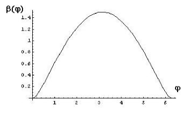
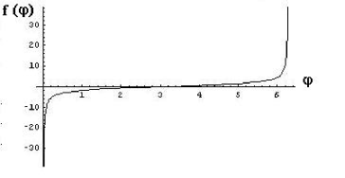
Figure 3: Upper plot: the function $\beta(\varphi)$, representing the ”speed” ${\rm d}\varphi/{\rm d}z$ (in terms of the effective dynamics description provided by (5.4)) of the (1,0) soliton in adimensional units (see text and (5.7)), for $\lambda=3/4$. Lower plot: the function $f(\varphi)=\int[1/\beta(\varphi)]{\rm d}\varphi$,to be inverted in order to get the (1,0) soliton solution (see 5.11)), again for $\lambda=3/4$; here $c_{0}$ has been chosen according to (5.10), so that $f(\pi)=0$.

Needless to say, integrating also the right hand side of (5.7), we get $f(\varphi)=B(z-z_{0})$. With $z_{0}=0$ (this integration constant can be absorbed in $c_{0}$), this yields finally for the (1,0) solution (shown graphically in fig.3)

$$\varphi\ =\ f^{-1}(Bz)\ .$$

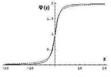
Figure 4: The (1,0) soliton for the Yakushevich model without the contact approximation, see (5.11), with $\lambda=3/4$ (solid lines); and for the Yakushevich model with the contact approximation (dotted lines). Here $\varphi$ is in units of $\pi$, and $z$ in units of the distance $\delta$ between successive base pairs.

V.2 The (0,1) solution

For the (0,1) solution we can set $\varphi=0$, which means $\vartheta_{2}=-\vartheta_{1}$. With this, and writing again $r=\lambda A$,

$$(\ell-\ell_{0})^{2}\ =\ 4\ A^{2}\ \lambda^{2}\ \left(1-\cos\eta\right)^{2}\ .$$

The effective potential is hence given by

$$Q(\eta)=W(0,\eta)={V(0,\eta)\over 2\mu}={(A\lambda)^{2}K_{p}\over\mu}(1-\cos\eta)^{2}\ .$$

Note that again $\mu<0$ implies $Q(\eta)\leq 0$ for all $\eta$, and that $Q(0)=0$. Conservation of energy provides in this case ${\rm d}\eta/{\rm d}z=\sqrt{-2Q(\eta)}$; hence we have

$${{\rm d}\eta\over{\rm d}z}\ =\ \lambda\,B\,(1-\cos\eta)$$

with $B$ as above. Equation (5.14) is immediately integrated, providing

$${\rm ctg}(\eta/2)\ =\ -\,\lambda\,B\,(z-z_{0})\ .$$

We can choose $z_{0}=0$, so that $\eta(\pi)=0$, and $\eta$ is antisymmetric with respect to $z=0$. In conclusion, the (0,1) solution is given by

$$\begin{array}[]{rl}\eta=&-2\,{\rm arcctg}(\lambda Bz)\ =\\ =&2\,\left[\pi-\arccos\left({\lambda Bz\over\sqrt{1+\lambda^{2}B^{2}z^{2}}}\right)\right]\ ;\end{array}$$

this is shown in fig.4. Note that some care should be taken in using appropriate determination of the ${\rm arcctg}$ and $\arccos$ functions so that $\eta$ is continuous at $z=0$.

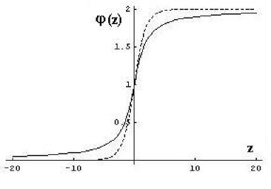
Figure 5: The (0,1) soliton for the Yakushevich model without the contact approximation, see (5.5), with $\lambda=3/4$ (solid lines); and for the Yakushevich model with the contact approximation (dotted lines); units as in fig.3.

V.3 Comparison with standard Y solitons

The standard Yakushevich model predictions are recovered for $r=A$, i.e. for $\lambda=1$. The solitons shape is evidently very similar to those of standard Yakushevich solitons also for $\lambda\not=1$, see figs.3 and 4.

In order to compare more precisely the results obtained within and without the contact approximation, we recall that with the contact approximation the (1,0) and (0,1) Yakushevich solitons are given respectively by GRPD ; YakuBook

$$\begin{array}[]{lr}\varphi(z)\ =\ 4\,\arctan\,[e^{Bz}]&,\eta=0\ ;\\ \eta(z)\ =\ 2\,\arccos\,\left[-Bz/\sqrt{1+B^{2}z^{2}}\right]&,\varphi=0\ .\end{array}$$

As for the soliton width, which represents the size of the transcription bubbles in the Englander et al. theory, this can be determined exactly via (5.9) and (5.15) once we decide how this should be measured. That is, the width will correspond to $z_{+}-z_{-}$ where $z_{\pm}$ are the points at which the angles $\varphi$ or $\eta$ differ by their asymptotic value ($0$ or $2\pi$) by less than a given amount $\Delta$. This is shown in fig.5 for small values of $\Delta$.

It should be stressed that the soliton widths vary quite slowly with $\lambda$; thus, the predictions of the model will not sensitively depend on the precise value of $\lambda$.

More precisely, these are given by the parameter $B^{-1}$, which – see (5.8) – is written as

$$B^{-1}\ =\ (\lambda/2)\ \sqrt{|\mu|/(K_{p}r^{2})}\ ;$$

again we stress that the curves plotted in fig.5 have a not so steep slope, which shows that the predictions of the model do not depend too much on the precise value of $B$.

In the limit $v\to 0$ we have $|\mu|=K_{s}\delta^{2}$ and hence

$$B^{-1}\ =\ b\ \delta\ \ {\rm with}\ \ b\ =\ {\lambda\over 2}\,\sqrt{K_{s}\over K_{p}r^{2}}\ .$$

As clear from fig.5, dropping the contact approximation will cause a widening of the Yakushevich solitons; this goes in the right direction since the standard Yakushevich model produces the right order of magnitude for the soliton width but with a too small exact numerical value GaeJBP .

Indeed, it is experimentally known that the transcription bubbles have a width of about 15–20 base pairs; this is the size of the region in which the base pairs are open and the base sequence can be accessed by the RNA Polymerase. It is not easy to assess what is precisely the angle at which base pairs should be considered as open, so we have plotted different possibilities in fig.5.

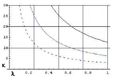
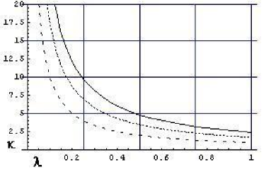
Figure 6: Half-width for the (1,0) soliton (upper) and the (0,1) soliton (lower) for the Yakushevich model without the contact approximation. The curves show the half-width $\kappa$ (in units of $B^{-1}=b\delta$) of the solitons as functions of $\lambda$, with different conventions for the measure of the half-width itself, see text: $\Delta=\pi/20$ (continuous curves), $\Delta=\pi/10$ (dotted curves) and $\Delta=\pi/5$ (dashed curves).

VI Conclusions and outlook

We have considered the Yakushevich model beyond the contact approximation $\ell_{0}\to 0$, focusing on the solitonic excitations which – according to Englander et al. – are supposed to play a functional role in the transcription process.

We have shown that in this case soliton solutions are still present, and can be described exactly in analytical terms; the simple form obtained within the contact approximation is replaced by a more complex expression, involving elliptic integrals. However, the qualitative form of soliton solutions is little changed, and their width is only very moderately increased.

This shows that the Yakushevich model is actually quite robust against changes in $\ell_{0}$ and dropping of the contact approximation; this not really for what concerns its mathematical aspects, but rather for what concerns its physical features and predictions, in particular in the fully nonlinear regime.

Thus, the first outcome of our work is that one is physically quite justified in considering the simplifying contact approximation in the Yakushevich model, albeit the analysis can be performed with the same completeness without that approximation.

Let us mention that other work in progress CDG show that by considering a more detailed description – in various ways – of the DNA molecule, one obtains indeed new features with respect to simple idealized models as the Yakushevich one.

In this respect, the present work suggests that in analyzing these more detailed – and hence more difficult to study – models one can in the first instance adopt the same kind of approximation adopted by Yakushevich in her original study, and focus instead on other features of the model. This suggestion will be taken up in forthcoming work CDG .

Appendix. Dispersion relations

In this note we are mainly interested in solitonic excitations, hence fully nonlinear dynamics. However, the study of small amplitude excitations has some interest, both per se and in order to emphasize how crucial the contact approximation is in this regime.

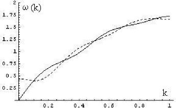
	(a)
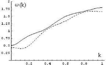
	(b)
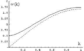
	(c)

Figure 7: Dispersion relations for different versions of the Yakushevich model. (a): The dispersion relations for $\omega=\omega(k)$ as described by (A.3) for the helicoidal Y model without the contact approximation. (b): Dispersion relations for the standard (i.e. $\ell_{0}=0$) Y model with helicoidal terms. (c): Dispersion relations for the standard Y model without helicoidal terms. In all plots, the continuous line refers to the $\psi$ branch, the dashed one to the $\chi$ branch. We have used the values $K_{s}=0.13{\rm eV/rad}^{2}$, $K_{h}=0.009{\rm eV/rad}^{2}$ GaeJBP ; here $k$ is given in units of $\pi/\delta$, and $\omega$ in ${\rm ps}^{-1}$. The $\chi$ branch of the standard Y model without helicoidal terms (plot on the right) coincides with the degenerate dispersion relations of the Y model without the contact approximation and without helicoidal terms.

Small amplitude dynamics around the equilibrium position $\psi_{n}=\chi_{n}=0$ is described by the linearization of (1.10) at $(0,0)$. As $V_{0}$, hence $V$, is non quadratic there, these collapse to a pair of identical equations for $\psi$ and $\chi$. In particular, the dispersion relations are now completely degenerated, and the intrapair term has no role in them.

This degeneration is removed by introducing in the model the “helicoidal” terms mentioned in sect.1 Dauhel ; Gaehel ; GRPD . This amounts to introducing in the Lagrangian a new potential term

$$U_{h}\ =\ {K_{h}\over 2}\ \sum_{i}\left[\left(\vartheta^{(1)}_{i+p}-\vartheta^{(2)}_{i}\right)^{2}\,+\,\left(\vartheta^{(2)}_{i+p}-\vartheta^{(1)}_{i}\right)^{2}\right]\ .$$

Here $p$ is the half-pitch of the helix in nucleotide units; it takes the value $p=5$ in B-DNA.

The introduction of this terms in $L$ entails that a new term should be added to the right hand side of the Euler-Lagrange equations (1.10); this new term is linear and thus is also present in their linearization.

With standard computations, the new linearized equations are (note the sign differences in the new terms)

$$\begin{array}[]{rl}I{\ddot{\psi}}_{n}\ =&\ K_{s}\,\left(\psi_{n+1}-2\psi_{n}+\psi_{n-1}\right)\ +\\ &+\ K_{h}\,\left(\psi_{n+p}-2\psi_{n}+\psi_{n-p}\right)\ ,\\ I{\ddot{\chi}}_{n}\ =&\ K_{s}\,\left(\chi_{n+1}-2\chi_{n}+\chi_{n-1}\right)\ +\\ &-\ K_{h}\,\left(\chi_{n+p}+2\chi_{n}+\chi_{n-p}\right)\ .\end{array}$$

Passing to the continuum approximation and Fourier transforming via $\Phi(x,t)=f_{k\omega}\exp[i(kx+\omega t)]$, $\Xi(x,t)=g_{k\omega}\exp[i(kx+\omega t)]$, the above yield

$$\begin{array}[]{rl}\omega^{2}_{\psi}=&(2K_{s}/I)[1-\cos(k\delta)]+(2K_{h}/I)[1-\cos(kp\delta)]\\ \omega^{2}_{\chi}=&(2K_{s}/I)[1-\cos(k\delta)]+(2K_{h}/I)[1+\cos(kp\delta)]\end{array}$$

for the $\psi$ and the $\chi$ branch respectively (note that here the continuous wave number $k$ has the dimension of $[L]^{-1}$, and the lattice spacing $\delta$ sets the space scale; one could of course also pass to a dimensionless wave number $\kappa=k\delta$). These are the dispersion relations – plotted in fig.5a – for the helicoidal Yakushevich model without the contact approximation. Note that a nonzero $\ell_{0}$ causes the presence, even in the helicoidal case, of phonon modes (contrary to the $\ell_{0}=0$ case).

For comparison purposes, we note that the dispersion relations for the standard Yakushevich model are

$$\begin{array}[]{rl}\omega^{2}_{\psi}=&(2K_{s}/I)[1-\cos(k\delta)]+(2K_{h}/I)[1-\cos(kp\delta)]+\\ &+2K_{p}r^{2}/I\\ \omega^{2}_{\chi}=&(2K_{s}/I)[1-\cos(k\delta)]+(2K_{h}/I)[1+\cos(kp\delta)]\end{array}$$

(the non-helicoidal case is obtained setting $K_{h}$ in the above); these are plotted in fig.5b, and in fig.5c for the non-helicoidal ($K_{h}=0$) case.

Quantities of physical interest are readily evaluated, at least numerically, from (A.3). For $K_{h}\not=0$, the $\chi$ branch has a nontrivial minimum; this is reached for $k=k_{0}=0.101\AA^{-1}$, i.e. for $\lambda=\lambda_{0}=62\AA=18\delta$. It is suggestive to remark that if solitons grow out of oscillations triggered by thermal excitations, and assuming equipartition of energy between Fourier modes, the larger amplitude excitations have a characteristic size which is of the order of the size of the transcription bubble, the latter being $15-20$ base pairs GRPD ; YakuBook . To the above value of $k_{0}$ corresponds a frequency $\omega_{0}=0.4{\rm ps}^{-1}$, i.e. a period of oscillations $T_{0}\simeq 16{\rm ps}$; typical values for $T_{0}$ observed in experiments are in the picoseconds range.

The speed of phonon excitations $v_{s}$ corresponds to $d\omega_{\psi}(k)/dk$ for $k\to 0$. In the $\ell_{0}=0$ case, with the values of parameters given above, we get $v_{s}\simeq 280$m/s, while if we drop the contact approximation we get $v_{s}\simeq 470$m/s. These values should be compared with experimental observations for the speed of torsional waves, which provide values in the range of $v_{s}=1.6\pm 0.3$ Km/s YakuBook .

References

- (1) M. Barbi, S. Cocco and M. Peyrard, “Helicoidal model for DNA opening”, Phys. Lett. A 253 (1999), 358-369
- (2) M. Barbi, S. Cocco, M. Peyrard and S. Ruffo, “A twist-opening model of DNA”, J. Biol. Phys. 24 (1999), 97-114
- (3) M. Barbi, S. Lepri, M. Peyrard and N. Theodorakopoulos, “Thermal denaturation of a helicoidal DNA model”, Phys. Rev. E 68 (2003), 061909
- (4) R.K. Bullough, P.J. Caudrey and H.M. Gibbs, “The double sine-Gordon equations”, pp. 107-141 in Solitons (R.K. Bullough and P.J. Caudrey eds.), Springer (Berlin) 1980
- (5) M. Cadoni, R. De Leo and G. Gaeta, “A composite Y model of DNA dynamics”, preprint q-bio.BM/0604014 (2006)
- (6) C. Calladine and H. Drew, Understanding DNA, Academic Press (London) 1992; C. Calladine, H. Drew, B. Luisi and A. Travers, Understanding DNA ( edition), Academic Press (London) 2004
- (7) F. Calogero and A. Degasperis, Spectral Transform and Solitons: tools to solve and investigate nonlinear evolution equations, North-Holland (New York) 1982
- (8) Th. Dauxois, “Dynamics of breather modes in a nonlinear helicoidal model of DNA”, Phys. Lett. A 159 (1991), 390-395
- (9) S.W. Englander, N.R. Kallenbach, A.J. Heeger, J.A. Krumhansl and A. Litwin, “Nature of the open state in long polynucleotide double helices: possibility of soliton excitations”, PNAS USA 77 (1980), 7222-7226
- (10) G. Gaeta, “On a model of DNA torsion dynamics”, Phys. Lett. A 143 (1990), 227-232
- (11) G. Gaeta, “Results and limits of the soliton theory of DNA transcription”, J. Biol. Phys. 24 (1999), 81-96
- (12) G. Gaeta, C. Reiss, M. Peyrard and Th. Dauxois, “Simple models of non-linear DNA dynamics”, Rivista del Nuovo Cimento 17 (1994) n.4, 1–48
- (13) J.A. Gonzalez and M. Martin-Landrove, “Solitons in a nonlinear DNA model”, Phys. Lett. A 191 (1994), 409-415
- (14) Y. Kafri, D. Mukamel and L. Peliti, “Why is the DNA denaturation transition first order?”, Phys. Rev. Lett. 85 (2000), 4988-4991; “Melting and unzipping of DNA”, Eur. Phys. J. B 27 (2002), 135-146
- (15) M. Peyrard, “Nonlinear dynamics and statistical physics of DNA”, Nonlinearity 17 (2004) R1-R40
- (16) M. Peyrard and A.R. Bishop, “Statistical mechanics of a nonlinear model for DNA denaturation”, Phys. Rev. Lett. 62 (1989), 2755-2758
- (17) M. Volkenstein, Biophysique, MIR (Moscow) 1985
- (18) L.V. Yakushevich, “Nonlinear DNA dynamics: a new model”, Phys. Lett. A 136 (1989), 413-417
- (19) L.V. Yakushevich, “Nonlinear DNA dynamics: hyerarchy of the models”, Physica D 79 (1994), 77-86
- (20) L.V. Yakushevich, Nonlinear Physics of DNA, Wiley (Chichester) 1998; second edition 2004
- (21) L.V. Yakushevich, A.V. Savin and L.I. Manevitch, “Nonlinear dynamics of topological solitons in DNA”, Phys. Rev. E 66 (2002), 016614
- (22) F. Zhang and M.A. Collins, “Model simulations of DNA dynamics”, Phys. Rev. E 52 (1995), 4217-4224