We describe a mechanism for pronounced biochemical oscillations, relevant to microscopic systems, such as the intracellular environment. This mechanism operates for reaction schemes which, when modeled using deterministic rate equations, fail to exhibit oscillations for any values of rate constants. The mechanism relies on amplification of the underlying stochasticity of reaction kinetics within a narrow window of frequencies. This amplification allows fluctuations to “beat the central limit theorem,” having a dominant effect even though the number of molecules in the system is relatively large. The mechanism is quantitatively studied within simple models of self-regulatory gene expression, and glycolytic oscillations.

I Introduction

Biochemical oscillations have been studied from complementary experimental and theoretical perspectives for many years. They appear to be generic processes in biological systems, with numerous examples known in both epigenetic and metabolic contexts [1-4]. Well known instances are circadian rhythms (e.g. in microorganisms [5,6]), and the oscillation of ATP and ADP concentrations during phosphorylation of fructose-6-phosphate (F6P), a key step in glycolysis [7,8]. The study of biochemical oscillations has benefited from an intimate collaboration between experimentalists and theorists: reaction networks are pieced together in the laboratory, with hypotheses severely constrained by results from mathematical models [4,8]. These mathematical models are generally constructed using deterministic chemical rate equations. Within this modeling framework, the signature of oscillatory behavior is the existence of a limit cycle. The absence of a limit cycle is assumed to imply that the underlying reaction scheme, upon which the model is based, does not have cyclic behavior. Recently, a number of groups have challenged this assumption [9-12], mainly in the context of calcium oscillations. They have studied deterministic rate equations which support a limit cycle over a certain range of parameter values, and have found, from computer simulations, that the addition of noise can expand the region of parameter space in which cycles occur. These authors demonstrate that this effect can be maximized for particular values of the system size or noise strength. On this basis, the effect has been termed “internal noise stochastic resonance.” We show here that internal noise can have a far more profound effect on biochemical reaction kinetics; namely, inducing amplified oscillations in systems which, when modeled with rate equations, lack a limit cycle throughout their entire parameter space. Thus, from the view of conventional deterministic modeling, these reaction schemes would be immediately ruled out as candidates to describe biochemical oscillations.

In this paper we develop a theoretical framework, using the Van Kampen system-size expansion [13-15], which allows an exact analytic description of these stochastically induced cycles – indeed, our theory reduces to a problem in linear algebra regardless of the reaction scheme under study, thereby allowing straightforward analysis. A crucial point is that this effect operates only in systems composed of a relatively modest number of molecules – typically in the range $10^{2}-10^{6}$. Many biochemical reactions within cells operate with numbers of molecules in this range, which leads us to believe that intracellular processes may well exploit this amplification mechanism. Our result is at odds with the intuitive notion that fluctuations can be safely ignored for systems composed of many thousands of molecules – the reason being that, here, the amplitude of fluctuations is composed of two factors: the usual statistical factor $1/\sqrt{N}$ (where $N$ is the typical number of molecules in the system), and a large factor $R\gg 1$ arising from the amplification of the underlying noise. If $R/\sqrt{N}\sim O(1)$ or larger, the intuitive conclusion that fluctuations can be ignored for $N\gg 1$, is incorrect.

For ease of presentation we shall introduce this mechanism through two relatively simple examples – one epigenetic (gene regulation), the other metabolic (glycolysis). Generalizations to more complex reaction schemes is straightforward, since, as already mentioned, the analysis of fluctuations reduces to an exercise in linear algebra. We will develop the theoretical ideas using the language of the gene regulation model (defined in Figure 1a) for concreteness, because it involves only the populations of two constituents, unlike the model of glycolytic oscillations which involves four.

The outline of the remainder of this paper is as follows. In section II we introduce the urn model representation of the gene regulation model, and proceed to instantiate this as a master equation. The deterministic limit of the master equation is derived in section III, and is shown to correspond to the usual chemical rate equation description. We calculate the effect of weak fluctuations in section IV, using the Van Kampen system-size expansion. We obtain a description of the fluctuations as a set of linear stochastic differential equations, which can therefore be analyzed exactly. The power-spectra obtained from these equations have resonance peaks which considerably enhance the $1/\sqrt{N}$ effects we would naively expect from fluctuations. The analysis (master equation, deterministic limit, first-order fluctuations) is repeated in a condensed form for Selkov’s model of glycolysis in section V. Again, we find a strong peak in power spectrum of the fluctuations indicating amplified oscillations. We end with a discussion of our results in the broader context of biochemical reaction networks.

II Individual-based stochastic model for the gene regulation model

Consider, first, a simple reaction scheme in which an enzyme inhibits the transcription of its parent gene (Figures 1a and 1b). More elaborate reaction schemes based on this simple model have long been proposed to explain circadian rhythms [5,16]. It is well-known that a deterministic model of this simplest reaction scheme involving two chemical agents (mRNA and the enzyme) will fail to produce cycles – at least three chemical agents (the mRNA, the enzyme, and an intermediate form, e.g. the primary RNA transcript) are required. It is important to recall that the deterministic model is an approximate representation of the actual chemical kinetics – it is strictly accurate for an infinite bath of molecules which are well-mixed. In order to describe a finite number of molecules it is necessary to use a discrete stochastic formulation in which one tracks the probability distribution of chemical concentrations over time. We have developed a standard stochastic treatment of the two-agent reaction scheme in Figures 1a and 1b. The calculational steps used in the approach are illustrated in a flow-chart (Figure 2). By taking the limit of the number of molecules in our system, $N$, to be infinite, we indeed recover the deterministic theory – this is an important benchmark. To handle the case of a finite number of molecules, we perform a system size expansion [13], which is a standard technique from the theory of stochastic processes, in which fluctuations are accounted for within a perturbative treatment. The second order terms in this expansion describe the fluctuations about the deterministic theory. These fluctuations satisfy linear equations and their statistics can be solved exactly. In particular, we calculate the power spectrum of these fluctuations. We find that for a wide range of parameters, the power spectrum has a pronounced maximum within a narrow window of frequencies.

In order to perform systematic numerical comparisons between integrating the rate equations and simulating the stochastic model it is convenient to envisage the reactions (Figures 1a and 1b) occurring within two baths, as shown in figure 3a. The empty state $\emptyset$ has been replaced by null constituents $E_{1}$ and $E_{2}$ to be discussed further below. The reason for introducing two baths is simply because it is easier to set up the dynamics of the system and is closer in spirit to other systems (grounded in population dynamics) which have been analyzed in a similar way, and are well-understood [14,15].

Our aim is to build an individual-based stochastic model, and so the basic ingredients will be the number of $M$ (mRNA) and $E_{1}$ (null) constituents in bath 1 and of $P$ (enzyme) and $E_{2}$ (null) constituents in bath 2 — in a given stochastic realization at a given time $t$. The dynamics will consist of picking constituents from the baths at each time step and attempting the specified reactions. Performing many runs of such reactions will enable us to collect a large number of realizations and extract average behavior. The reactions proceed according to the rates shown in Figure 3a, and if the selection of constituents does not correspond to one of the four reactions, then the molecules are returned to their respective baths without any action being taken.

On the basis of the specification so far, and summarized in Figure 3a, numerical simulations of the model can be carried out. We use the elegant Gillespie algorithm [17] which uses the information encoded in the reaction scheme to generate random time increments, in each of which a randomly selected reaction is forced to occur. The time increments and reactions are selected according to weighted distributions in such a way that the probability distribution of the stochastic time series generated is exact. The results of some of these simulations are displayed in Figures 4 and 5.

It is also possible to derive a set of equations which describe the stochastic process which is defined by the model we have specified. To do this, we first note that there has been an implication that the choice of constituents at a given time step is a random process, only dependent on the numbers of the various molecules in the baths at that time, and not on choices or availability at previous time steps. Assumptions of this kind imply that the process is Markov, and so can be modeled using a master equation [13,18]. This is essentially a continuous time version of a Markov chain. Before we can write down this equation, we need to define some more quantities.

Let us denote the number of molecules of the various kinds as follows: in bath 1 the number of molecules of $M$ is $n_{1}$ and in bath 2 the number of molecules of $P$ is $n_{2}$. The state of the system is then denoted by the two numbers $(n_{1},n_{2})$. We will frequently write this as $\underline{n}$ when we simply want to refer to the general state of the system. Note that we do not confer the status of independent variables on the numbers of $E_{1}$ or $E_{2}$ constituents. If we denote the total number of constituents in bath 1 by $N_{1}$ and that in bath 2 by $N_{2}$, then the number of $E_{1}$ and $E_{2}$ constituents are simply what is required to make up these numbers: $(N_{1}-n_{1})$ $E_{1}$ and $(N_{2}-n_{2})$ $E_{2}$ constituents. This is why it was necessary to introduce the null constituents: if they had not been included, the number of $M$ and $P$ molecules would not have the freedom to vary — they provide room for independent changes in the numbers of both $M$ and $P$ molecules.

We may now define transition rates from one state, $\underline{n}$, to a different state $\underline{n}^{\prime}$. For instance, in the fourth reaction, the number of $P$ molecules increases by 1 (recall that the number of $E_{2}$ molecules is not an independent variable). So in this case, $\underline{n}=(n_{1},n_{2})$ and $\underline{n}^{\prime}=(n_{1},n_{2}+1)$. We denote the transition rate by $T(\underline{n}^{\prime}|\underline{n})$. In our convention, initial states are on the right and final states on the left. When picking the constituents, there is a probability of $n_{1}/N_{1}$ of $M$ being chosen, $(N_{2}-n_{2})/N_{2}$ that an $E_{2}$ is chosen, and the reaction happens at a rate $k_{2}$. This gives the result $k_{2}(n_{1}/N_{1})(N_{2}-n_{2})/N_{2}$ for this particular transition rate. Others may be found in the same way. A complete listing with $\underline{n}=(n_{1},n_{2})$ is

• $M\stackrel{{\scriptstyle\mu_{1}}}{{\longrightarrow}}E_{1}$,  $\underline{n}^{\prime}=(n_{1}-1,n_{2})$,

  $$T(\underline{n}^{\prime}|\underline{n})=\mu_{1}\frac{n_{1}}{N_{1}}\,.$$

• $P\stackrel{{\scriptstyle\mu_{2}}}{{\longrightarrow}}E_{2}$,  $\underline{n}^{\prime}=(n_{1},n_{2}-1)$,

  $$T(\underline{n}^{\prime}|\underline{n})=\mu_{2}\frac{n_{2}}{N_{2}}\,.$$

• $E_{1}\stackrel{{\scriptstyle k_{1}}}{{\longrightarrow}}M$,  $\underline{n}^{\prime}=(n_{1}+1,n_{2})$,

  $$T(\underline{n}^{\prime}|\underline{n})=k_{1}\frac{(N_{1}-n_{1})}{N_{1}}=k_{0}\exp{\left(-\lambda n_{2}/N_{2}\right)}\,\frac{(N_{1}-n_{1})}{N_{1}}\,.$$

• $M+E_{2}\stackrel{{\scriptstyle k_{2}}}{{\longrightarrow}}M+P$,  $\underline{n}^{\prime}=(n_{1},n_{2}+1)$,

  $$T(\underline{n}^{\prime}|\underline{n})=k_{2}\frac{n_{1}}{N_{1}}\frac{(N_{2}-n_{2})}{N_{2}}\,.$$

Note, we use an exponential function $\exp(-\lambda{\rm[P]})$ to model the down-regulation of transcription. The primary reason is this form introduces one extra parameter ($\lambda$) into the model, unlike the typical Hill form [16] $(1+\alpha{\rm[P]}^{q})^{-1}$ which introduces two new parameters ($\alpha$ and $q$). Furthermore, in deterministic studies (albeit using more complex three-component models), it is found that large values of $q$ ($\sim 10$) are required for limit cycles to occur [16]. For such large values of $q$, the Hill form is a rapidly decaying function, and it seems reasonable to replace it by a simple exponential function.

Having defined the transition rates, we are now in a position to write down the master equation. It has the general form [13,18]

$$\frac{d}{dt}P(\underline{n},t)=\sum_{\underline{n}^{\prime}\neq\underline{n}}\,T(\underline{n}|\underline{n}^{\prime})P(\underline{n}^{\prime},t)-\sum_{\underline{n}^{\prime}\neq\underline{n}}\,T(\underline{n}^{\prime}|\underline{n})P(\underline{n},t)\,,$$ (1)

where $P(\underline{n},t)$ is the probability that the system is in the state $\underline{n}$ at time $t$. This equation has a simple interpretation: the first term on the right hand side is the sum of the transition rates into the state $\underline{n}$ from all other states $\underline{n}^{\prime}$ and the second term is the sum of the transition rates out of the state $\underline{n}$ into all other states $\underline{n}^{\prime}$. When the second term is subtracted from the first, it gives the rate of change of the probability $P$.

So far we have formulated a discrete stochastic model and given specified analytic forms for transition probabilities between states, which can be used in conjunction with the master equation (1) to, in principle, solve for the probability, $P(\underline{n},t)$, that the system is in state $\underline{n}$ at time $t$. We will now start from the master equation and (i) determine the form that the model takes in the mean-field limit, and (ii) implement the system-size expansion to study the origin of the cycling behavior, which is absent in the deterministic (mean-field) limit.

III The deterministic limit

A straightforward way of obtaining the deterministic version of the model, valid in the limit of very large system size, from the master equation is to multiply (1) by $n_{1}$ and $n_{2}$ in turn and to sum over all the states. This generates rate equations which are the deterministic equations if correlations between the variables are ignored. Let us illustrate the method in the case of $n_{2}$. We wish to calculate $\langle n_{2}\rangle=\sum_{\underline{n}}n_{2}P(\underline{n},t)$ by multiplying the master equation by $n_{2}$ and summing over $\underline{n}$. On the left-hand side we find $d\langle n_{2}\rangle/dt$. On the right-hand side are two terms which are nearly equal and opposite — if it was not for the $n_{2}$ factor, they would be. The only difference between the two terms is that $\underline{n}$ and $\underline{n}^{\prime}$ are interchanged. So if $n_{2}$ does not change in a reaction, as for reactions 1 and 3, then the two contributions do in fact cancel out. If it decreases by 1, as in reaction 2, then a shift in the sum over $n_{2}$ gives an overall contribution of $-1$, and if it increases by 1, as in the reaction 4, then a shift in the sum over $n_{2}$ the other way, gives an overall contribution of $+1$. This gives the result

$$\frac{d}{dt}\langle n_{2}\rangle=-\mu_{2}\left\langle\frac{n_{2}}{N_{2}}\right\rangle+k_{2}\left\langle\frac{n_{1}}{N_{1}}\frac{(N_{2}-n_{2})}{N_{2}}\right\rangle\,.$$

So far this is exact. The mean-field approximation enters through ignoring correlations, which vanish as $N_{1},N_{2}\to\infty$. So, for example, this means that $\langle n_{i}n_{j}\rangle=\langle n_{i}\rangle\langle n_{j}\rangle$ for $i,j=1,2$. If we make this approximation and introduce the fractions of $M$ and $P$ to be $\phi_{1}$ and $\phi_{2}$ respectively, in the limit $N_{1},N_{2}\to\infty$, then we find

$$\frac{d\phi_{2}}{dt}=-\frac{\mu_{2}}{N_{2}}\phi_{2}+\frac{k_{2}}{N_{2}}\phi_{1}\left(1-\phi_{2}\right)\,.$$

This is the required deterministic equation. So in summary, if we define $\phi_{i}=n_{i}/N_{i}$ and scale the time by introducing $\tau=t/N_{1}$, then the deterministic equations corresponding to the individual based stochastic model we have defined are

$$\frac{d\phi_{1}}{d\tau} = -\mu_{1}\phi_{1}+k_{0}\exp{\left(-\lambda\phi_{2}\right)}\left(1-\phi_{1}\right)\,,$$ (2)

$$\sigma^{-1}\,\frac{d\phi_{2}}{d\tau} = -\mu_{2}\phi_{2}+k_{2}\phi_{1}\left(1-\phi_{2}\right)\,,$$ (3)

where $\sigma=N_{1}/N_{2}$. Note that the mean-field approximation as applied to the first equation implies that $\langle\exp{\left(-\lambda n_{2}/N_{2}\right)}\rangle=\exp{\left(-\lambda\langle n_{2}\rangle/N_{2}\right)}$.

Most of the theoretical investigations of biochemical reactions start from a set of differential equations of the type (2) and (3). One of the first quantities of interest in such studies are the fixed points of the system. If we denote the fixed points with an asterisk and define $X=\lambda\phi^{*}_{2}$, then $X$ satisfies the transcendental equation

$$k_{0}\,e^{-X}=\frac{\mu_{1}\mu_{2}X}{k_{2}\lambda-(k_{2}+\mu_{2})X}\,,$$ (4)

with the fixed points for $\phi_{1}$ given by

$$\phi^{*}_{1}=\frac{\mu_{2}X}{k_{2}(\lambda-X)}\,.$$ (5)

Note that $1-\phi^{*}_{1}>0$ and so the denominator of the right-hand side of Eq. (4) is never zero. Also, since the left-hand side of this equation is monotonically decreasing from its value at $X=0$ and the right-hand side is monotonically increasing from its value at $X=0$, it follows that there is always a unique solution for $X$ and therefore always just one fixed point. The condition $0\leq\phi^{*}_{2}\leq 1$ implies that $0\leq X\leq\lambda$, but the condition $0\leq\phi^{*}_{1}\leq 1$ gives the stronger constraint

$$X\leq\frac{k_{2}\lambda}{k_{2}+\mu_{2}}\,.$$ (6)

The stability of these fixed points would always be of interest, but the question takes on an added significance in our case, since the stability matrix associated with the non-trivial fixed point (Eqs. (4) and (5)) plays a central role in the analysis of the cycling phenomenon. To determine it, let us write the mean-field equations (2) and (3) in the form $d\phi_{i}/d\tau=f_{i}(\underline{\phi})$ where $i=1,2$. The fixed points are found from solving $f_{i}(\underline{\phi})=0$ and a linear stability analysis consists of writing $\phi_{i}=\phi_{i}^{*}+(\hat{\phi}_{i}/\sqrt{N_{i}})$, where the $\hat{\phi}_{i}$ are small deviations from the fixed point [19] . Note that we have included extra factors of $1/\sqrt{N_{i}}$ in the small deviations from the fixed point — which simply amounts to a re-scaling of $\hat{\phi}_{i}$ — compared to the usual linear stability analysis, so as to make contact with the system-size expansion in the next section. Linearizing about the fixed point gives $d\hat{\phi}_{i}/d\tau=\sum_{j}M_{ij}\hat{\phi}_{j}$, where $M_{ij}$ is defined by $M_{ij}=\partial f_{i}/\partial\phi_{j}|_{\rm FP}$. Here FP means “evaluated at the fixed point”. The explicit forms for the entries of the matrix $M$ are

$$M_{11} = -\mu_{1}-k_{0}\exp{\left(-\lambda\phi_{2}^{*}\right)}\,,$$

$$M_{12} = -k_{0}\lambda\sigma^{1/2}\exp{\left(-\lambda\phi_{2}^{*}\right)}\left(1-\phi_{1}^{*}\right)\,,$$

$$M_{21} = k_{2}\sigma^{1/2}\left(1-\phi_{2}^{*}\right)\,,$$

$$M_{22} = -\sigma\mu_{2}-\sigma k_{2}\phi_{1}^{*}\,.$$ (7)

These entries may be rewritten using the fixed-point equations to give

$$M_{11} = -\frac{\mu_{1}}{1-\phi^{*}_{1}}\,,\ \ \ M_{12}=-\lambda\mu_{1}\sigma^{1/2}\,\phi^{*}_{1}\,,$$

$$M_{21} = \mu_{2}\sigma^{1/2}\,\frac{\phi^{*}_{2}}{\phi^{*}_{1}}\,,\ \ M_{22}=-\sigma k_{2}\frac{\phi^{*}_{1}}{\phi^{*}_{2}}\,.$$ (8)

From these expressions it is clear that all entries of $M$ have a definite sign: $M_{11},M_{12}$ and $M_{22}$ are negative, and $M_{21}$ is positive. Therefore, the determinant and the trace of $M$ are positive and negative respectively for all parameter choices. This already tells us that the fixed point is stable, but further analysis is required if we wish to know whether or not the the fixed point is approached in an oscillatory fashion. This will be discussed again in the next section.

IV Analysis of the fluctuations

In contrast with the innate discreteness of the stochastic model, the mean-field equations involve functions of continuous variables. This is one of the reasons why they are more amenable to analytic treatment. It is the limit $N_{1},N_{2}\to\infty$ which leads to the continuity of the mean-field equations, as well as to the elimination of the fluctuations. In the section we will discuss how we can keep continuity, but still not lose the stochastic nature of the system. This is achieved by using new continuous variables $x_{1},x_{2}$ in place of the previously used discrete variables $n_{1},n_{2}$ to describe the probability distribution. The explicit form of the replacements are

$$\frac{n_{1}}{N_{1}}=\phi_{1}+\frac{x_{1}}{\sqrt{N_{1}}}\,,\ \ \ \frac{n_{2}}{N_{2}}=\phi_{2}+\frac{x_{2}}{\sqrt{N_{2}}}\,.$$ (9)

The $1/\sqrt{N}$ terms are present since, by the central-limit theorem, we expect fluctuations to be of the order of $1/\sqrt{N}$ when the variables $n_{1},n_{2}$ are expressed in terms of the fractions $n_{1}/N_{1}$ and $n_{2}/N_{2}$. As $N_{1},N_{2}\to\infty$, these fluctuations vanish, and the system is entirely described by the mean-field variables $\phi_{i}(\tau)$, which can be found, in principle, by solving Eqs. (2) and (3) with given initial conditions. If we imagine a plot of the probability distribution $P$ along the vertical axis, and the variables $n_{i}$ along the horizontal axes, for various values of $\tau$, then at the initial time $\tau=0$ $P$ is a delta-function spike at the starting values of the $n_{i}$. As $\tau$ increases, not only does the position of the peak move, but the probability distribution also broadens due to fluctuations. The $\phi_{i}(\tau)$, which are the solutions of Eqs. (2) and (3), tell us the position of the peak of the distribution and the variables $x_{i}(\tau)$ tell us something about the distribution itself. Actually it turns out that to order $1/\sqrt{N}$ (here we use $N$ to mean $N_{1}$ or $N_{2}$, since they are assumed to be of the same order), the probability distribution is Gaussian, and since the position of the peak is specified, all that is left to determine is the variance. Higher terms in the $1/\sqrt{N}$ expansion give deviations from the Gaussian form, which our numerical simulations show are very small for reasonable values of $N$. Once the leading (deterministic) contributions have been subtracted out from (9) (by, in effect, continuously moving the origin to the peak of the probability distribution) only fluctuations remain. If the $1/\sqrt{N_{1}}$ and $1/\sqrt{N_{2}}$ terms are then factored out, we may once again take $N\to\infty$. In this way the $x_{i}$ become continuous variables, and terms of different orders can be identified in the master equation.

The actual implementation of the system-size expansion is straightforward, if tedious. It is discussed clearly in [13] and in some detail in [14]. We shall illustrate it by applying it to one term in the master equation only. The reader should be able to understand the essential features of the method from this, and can then consult the above references to get a broader picture. Let us take reaction 2, in which the number of $P$ molecules decreases by 1. It gives a contribution to the term $T(\underline{n}^{\prime}|\underline{n})P(\underline{n},t)$ in the master equation (1) which is equal to $\mu_{2}(n_{2}/N_{2})P(n_{1},n_{2},t)$. It also gives a contribution to $T(\underline{n}|\underline{n}^{\prime})P(\underline{n}^{\prime},t)$ in the same equation which is equal to $\mu_{2}([n_{2}+1]/N_{2})P(n_{1},n_{2}+1,t)$. We can combine these two terms as follows:

$${\rm Reaction\ 2\ }:\ \ \ \left({\cal E}_{2}-1\right)\left[\mu_{2}\frac{n_{2}}{N_{2}}P(n_{1},n_{2},t)\right]\,,$$ (10)

where ${\cal E}_{2}$ is a step operator which is defined in terms of its action on functions of the $n_{i}$ by ${\cal E}_{2}^{\pm 1}\psi(n_{1},n_{2})=\psi(n_{1},n_{2}\pm 1)$. Similar operators can be defined for the other variables. The advantage of using these operators is that, within the replacement scheme (9), they have a simple form for large $N$. For example,

$${\cal E}_{2}^{\pm 1}=1\pm\frac{1}{\sqrt{N_{2}}}\frac{\partial}{\partial x_{2}}+\frac{1}{2N_{2}}\frac{\partial^{2}}{\partial x_{2}^{2}}+\ldots\,.$$ (11)

Substituting (9) and (11) in (10), and expanding in inverse powers of $\sqrt{N_{2}}$ one finds a contribution proportional to $1/\sqrt{N_{2}}$:

$$\frac{1}{\sqrt{N_{2}}}\,\mu_{2}\phi_{2}\,\frac{\partial\Pi}{\partial x_{2}}\,,$$ (12)

and a term of order $1/N_{2}$:

$$\frac{1}{N_{2}}\,\mu_{2}\left[\frac{\partial}{\partial x_{2}}\left(x_{2}\Pi\right)+\frac{1}{2}\,\phi_{2}\frac{\partial^{2}\Pi}{\partial x_{2}^{2}}\right]\,.$$ (13)

There are higher order terms, but this is as far as we need to go in the expansion. The quantity $\Pi$ which appears in Eqs. (12) and (13) is numerically equal to $P$, but is instead a function of the $x_{i}$ and of $t$. This means that the left-hand side of (1) now reads

$$\frac{\partial P}{\partial t} = \frac{\partial\Pi}{\partial t}-\sqrt{N_{1}}\frac{d\phi_{1}}{dt}\frac{\partial\Pi}{\partial x_{1}}-\sqrt{N_{2}}\frac{d\phi_{2}}{dt}\frac{\partial\Pi}{\partial x_{2}}$$ (14)

$$= \frac{1}{N_{1}}\frac{\partial\Pi}{\partial\tau}-\frac{1}{\sqrt{N_{1}}}\frac{d\phi_{1}}{d\tau}\frac{\partial\Pi}{\partial x_{1}}-\sigma^{-1}\frac{1}{\sqrt{N_{2}}}\frac{d\phi_{2}}{d\tau}\frac{\partial\Pi}{\partial x_{2}}\,.$$

Equating the right-hand side of the master equation (Eqs. (12) and (13)) to the left-hand side (Eq. (14)) order by order, we find that $\sigma^{-1}d\phi_{2}/d\tau$ has a contribution $-\mu_{2}\phi_{2}$ (the $\partial\Pi/\partial x_{2}$ cancel out) and

$$\frac{\partial\Pi}{\partial\tau}=\mu_{2}\sigma\left[\frac{\partial}{\partial x_{2}}\left(x_{2}\Pi\right)+\frac{1}{2}\,\phi_{2}\frac{\partial^{2}\Pi}{\partial x_{1}^{2}}\right]+\ldots\,,$$ (15)

where the dots mean that the reactions other than 2 will also give a contribution.

This partial, but explicit, calculation allows us to see more clearly how the expansion works. At leading order we have a contribution to the mean-field equation for $\sigma^{-1}d\phi_{2}/d\tau$ which is equal to $-\mu_{2}\phi_{2}$, which indeed appears in Eq. (3), and in none of the other mean-field equations. Therefore, an alternative, and in some sense more systematic, way of obtaining the mean-field equations is as the leading order terms in the large-$N$ expansion. The next-to-leading terms give a partial differential equation for the probability distribution $\Pi(\underline{x},t)$ which, when we include all the other reactions, has the form

$$\frac{\partial\Pi}{\partial\tau}=-\sum_{i}\,\frac{\partial}{\partial x_{i}}\left(A_{i}(\underline{x})\,\Pi\right)+\frac{1}{2}\sum_{i,j}\,B_{ij}\frac{\partial^{2}\Pi}{\partial x_{i}\partial x_{j}}\,.$$ (16)

From (15) we see that $A_{2}(\underline{x})=-\mu_{2}\sigma x_{2}+\ldots$ and $B_{11}=\mu_{2}\sigma\phi_{2}+\ldots$. In fact when all the reactions are included, the $A_{i}(\underline{x})$ remain linear functions of the $x_{j}$ and the $B_{ij}$ remain independent of them. We may therefore write

$$A_{i}(\underline{x})=\sum^{2}_{j=1}M_{ij}x_{j}\,.$$ (17)

This means that the probability distribution at next-to-leading order, $\Pi(\underline{x},\tau)$, is completely determined by two $2\times 2$ matrices: $M$ and $B$, whose elements are independent of the $x_{j}$, and only functions of the $\phi_{j}$. In fact it is a characteristic of the large-$N$ expansion that $M$ is nothing else but the Jacobian matrix with elements $\partial f_{i}/\partial\phi_{j}$, which may be calculated directly from the mean-field equations (2) and (3). If the initial transients have died away and the solution to the deterministic equations has approached a fixed-point $\underline{\phi}^{*}$, then $M$ will simply be the stability matrix at that fixed point. The stability matrix for the fixed point (4) and (5) is given in the previous section. The matrix $B$ has entries

$$B_{11} = \mu_{1}\phi_{1}+k_{0}\exp{\left(-\lambda\phi_{2}\right)}\left(1-\phi_{1}\right)$$

$$B_{22} = \mu_{2}\sigma\phi_{2}+k_{2}\sigma\phi_{1}\left(1-\phi_{2}\right)$$

$$B_{12} = B_{21}=0\,.$$ (18)

So, to summarize the position so far, we know the $M_{ij}$ and $B_{ij}$ in terms of the parameters which define the individually-based stochastic model, and therefore by solving Eq. (16) we can find all we need to know about the fluctuations for large $N_{1}$ and $N_{2}$. The partial differential equation (16) is a Fokker-Planck equation — a continuous version of the master equation — and can be solved, in principle, given the initial condition that $\Pi$ is a delta-function spike at $\tau=0$. In fact, for the simple case where the $B_{ij}$ are independent of $x_{j}$ and the $A_{i}$ are linear functions of the $x_{j}$, it can be solved exactly [13]. The result is a multi-variate Gaussian with $\langle x_{i}\rangle=0$, as already mentioned.

Our main aim in this paper is to understand oscillations and for this one of the main tools is Fourier analysis. The form of Eq. (16) is not so useful for this purpose, but fortunately there is a completely equivalent formulation of the stochastic process which is ideally suited to investigation using Fourier transforms. Rather than write an equation for the probability distribution function $\Pi$, an equation for the actual stochastic variables $x_{i}(\tau)$ can be given, in other words, the problem may be formulated as a set of stochastic differential equations of the Langevin type. The Langevin equations which are equivalent to (16) are [13]

$$\frac{dx_{i}}{d\tau}=A_{i}(\underline{x})+\eta_{i}(\tau)\,,$$ (19)

where $\eta_{i}(\tau)$ is a Gaussian noise with zero mean and with a correlation function given by

$$\langle\eta_{i}(\tau)\eta_{j}(\tau^{\prime})\rangle=B_{ij}\delta(\tau-\tau^{\prime})\,.$$ (20)

The system defined by Eqs. (19) and (20) is ideally suited to Fourier analysis, since the equations (19) are linear (since the $A_{i}$ are) and Eq. (20) implies that the noise is white, that is, the Fourier transform of its correlation function is frequency-independent.

Taking the Fourier transform of (19) gives

$$-i\omega\tilde{x}_{i}(\omega)=\sum^{2}_{j=1}M_{ij}\tilde{x}_{j}(\omega)+\tilde{\eta}_{i}(\omega)\,,$$ (21)

where the tilde denotes the Fourier transform. We may write this as

$$\sum^{2}_{j=1}\Phi_{ij}(\omega)\tilde{x}_{j}(\omega)=\tilde{\eta}_{i}(\omega)\,,\ \ \ \Phi_{ij}(\omega)\equiv-i\omega\delta_{ij}-M_{ij}\,.$$ (22)

The Fourier transform of $\eta_{i}(t)$ has the correlation function

$$\langle\tilde{\eta}_{i}(\omega)\tilde{\eta}_{j}(\omega^{\prime})\rangle=B_{ij}(2\pi)\delta(\omega+\omega^{\prime})\,.$$ (23)

From Eq. (22) we obtain $\tilde{x}_{i}(\omega)=\sum_{j}\Phi^{-1}_{ij}(\omega)\tilde{\eta}_{j}(\omega)$, and averaging the squared modulus of $\tilde{x}_{i}$ gives the power-spectra

$$P_{i}(\omega)=\langle|\tilde{x}_{i}(\omega)|^{2}\rangle=\sum^{2}_{j=1}\,\sum^{2}_{k=1}\,\Phi^{-1}_{ij}(\omega)B_{jk}\left(\Phi^{{\dagger}}\right)^{-1}_{ki}(\omega)\,,$$ (24)

where we have used $\Phi_{ij}(-\omega)=\Phi^{{\dagger}}_{ji}(\omega)$. [We have omitted the proportionality factor $2\pi\delta(0)$. In practice, when comparing the analytically calculated power spectra to those generated from a numerical time series, one uses a discrete Fourier transform, and the proportionality factor is simply equal to the time increment of the recorded values in the time series.]

To isolate the resonance, we note that $P_{i}(\omega)$ has the form of the ratio of two power series in $\omega$. The denominator, which will largely control the position of the resonance, can be simply expressed as the determinant of the matrix $\Phi$. If we define $D(\omega)=\det\Phi(\omega)$, then the denominator is just $|D(\omega)|^{2}$.

In Eqs. (21)-(24) we have written everything in a rather general form, since the formalism can be seen to generalize to the case of an arbitrary number of constituents rather easily, such as in the model of glycolysis in the next section which has 4 constituents. However, for the model we are presently considering, there are only two constituents and the expressions for $P_{i}(\omega),\ i=1,2$ have simple explicit forms:

$$P_{i}(\omega)=\langle|\tilde{x}_{i}(\omega)|^{2}\rangle=\frac{\alpha_{i}+\beta_{i}\omega^{2}}{|D(\omega)|^{2}}\,,$$ (25)

where $D(\omega)=-\omega^{2}+i\omega\,{\rm tr}M+\det M$ and where

$$\alpha_{1} = B_{11}M^{2}_{22}+B_{22}M^{2}_{12}\,,\ \ \ \beta_{1}=B_{11}\,,$$

$$\alpha_{2} = B_{11}M^{2}_{21}+B_{22}M^{2}_{11}\,,\ \ \ \beta_{2}=B_{22}\,.$$ (26)

Since the elements of the $M$ and $B$ matrices are known in terms of the parameters of the model and the fixed point values of the $\phi_{i}$, so are the $\alpha_{i}$ and $\beta_{i}$.

The denominator of the power spectrum in Eq. (25) is given by

$$|D(\omega)|^{2} = \left(\omega^{2}-\det M\right)^{2}+\left({\rm tr}M\right)^{2}\omega^{2}$$ (27)

$$= \left(\omega^{2}-\Omega^{2}_{0}\right)^{2}+\Gamma^{2}\omega^{2}\,,$$

where, since in Section III we found $\det M>0$ and ${\rm tr}M<0$, we have introduced $\Omega^{2}_{0}=\det M$ and $\Gamma=-{\rm tr}M$. So, we may write the power spectrum as

$$P_{i}(\omega)=\langle|\tilde{x}_{i}(\omega)|^{2}\rangle=\frac{\alpha_{i}+\beta_{i}\omega^{2}}{\left[\left(\omega^{2}-\Omega^{2}_{0}\right)^{2}+\Gamma^{2}\omega^{2}\right]}\,.$$ (28)

This form for the power-spectrum shows clearly the existence of a resonance: for a value of $\omega^{2}$ the denominator becomes small, and the power spectrum has a large peak centered on this frequency.

To analyze the nature of the resonance in more detail, let us set $z=\omega^{2}$ and ask for what values of $z$ the power spectrum (28) has a maximum. The condition $dP/dz=0$ gives

$$\beta z^{2}+2\alpha z+\left[\alpha\left(\Gamma^{2}-2\Omega^{2}_{0}\right)-\beta\Omega^{4}_{0}\right]=0\,,$$ (29)

where we have dropped the index $i$ on $\alpha_{i}$ and $\beta_{i}$. Let us begin by neglecting the term $\beta_{i}\omega^{2}$ in the numerator of Eq. (28) which may be justified for some parameter choices. Then the condition (29) simply becomes $z=(2\Omega^{2}_{0}-\Gamma^{2})/2$. Since we require $z=\omega^{2}>0$, this implies $2\Omega^{2}_{0}>\Gamma^{2}$. In terms of the stability matrix $M$, this condition reads $2\det M>({\rm tr}M)^{2}$, which implies that the eigenvalues of $M$ are complex. In the last section we showed that the eigenvalues of the stability matrix were either real and negative or complex with a negative real part. The condition that the power spectrum has an extremum imposes the latter.

In reality, the presence of the factor $\beta_{i}\omega^{2}$ in the numerator of the power spectrum may have a significant effect, and the full condition (29) has to be used. From Eqs. (18) and (26) we see that the $\alpha_{i}$ and $\beta_{i}$ are always positive, and so from Eq. (29) we see that the sum of the roots of this equation is negative and so at least one of the roots is negative. For the other one to be positive we require

$$\alpha\left(\Gamma^{2}-2\Omega^{2}_{0}\right)-\beta\Omega^{4}_{0}<0\,.$$ (30)

This is the general condition for an extremum of the power spectrum to occur. It goes beyond the the previous condition, which only involved the eigenvalues of the matrix $M$, since it contains the $\beta_{i}$ which come from consideration of the fluctuations about the fixed point. We may now ask if the extremum is a maximum. It is straightforward to show by calculating $d^{2}P/dz^{2}$ that, if a positive solution to Eq. (29) exists, then it is automatically a maximum.

A peak in the power spectrum indicates a resonant frequency, and a corresponding oscillation at this frequency. [We must stress that our use of the word “resonance” here follows the more general usage; namely, a peak in the power spectrum as a function of frequency. In “stochastic resonance” and its derivatives [9,11] (and references therein), the “resonance” refers to a maximized response of the system as a function of some parameter, such as the strength of the internal noise. Because of the potential for confusion, we often use the term “amplification” for the effect under consideration in this work.] The height of the peak indicates the strength of the amplification. The width of the peak indicates the amount of frequency dispersion one would observe about the resonant frequency. We have calculated the power spectra exactly for this epigenetic model. For a specific set of parameters, we show the power spectra for fluctuations in mRNA and enzyme concentrations (Figures 4c and 4d respectively). We have also computed stochastic realizations of time series for this reaction, using the exact Gillespie algorithm [17] (Figures 4a, b). Note, the resonant amplification $R$ for mRNA (defined as the height of the peak of the power spectrum relative to $P(0)$) is quite pronounced ($R\sim 30$), and, indeed, regular oscillatory peaks are easily discernible in the corresponding time series (Figure 4a). The constant dashed lines in Figures 4a, b are the results from the deterministic theory – which predicts a complete absence of cycling. We emphasize that there are two competing quantities which combine to determine the importance of these amplified oscillations – these are i) the relative height of the peak in the power spectrum $R$, and ii) the mean number of molecules in the system $N$. The amplitude of the oscillations in a time series measurement of the concentration will be of the order $R/\sqrt{N}$. This is why the effect dies away for macroscopic systems in which $N$ is extremely large. In the example given here $R\sim 30$ (for mRNA fluctuations), and so we can estimate that the oscillations will be negligible in intracellular systems for which $N_{\rm mRNA}\gg 1000$. Given the simplicity of this two component model, and the modest estimate above, this mechanism may be relevant to circadian rhythms in procaryotic cells, such as cyanobacteria [5], since such cells are small, and have no nuclear membrane separating transcription and translation processes (justifying, to some degree, a two-component model).

In Figure 5 we compare the exact form for the mRNA power spectrum, given above in (25), to a numerically generated power spectrum. The latter is computed from discrete Fourier transforms of a large number (10,000) of long (60,000 iterations) time series generated using the exact Gillespie algorithm described earlier. There is excellent agreement between the exact and numerical spectra, as expected.

V Selkov’s model of glycolysis

We now turn to an example from intracellular metabolic dynamics. Consider the key step in glycolysis in which the enzyme PFK1 catalyzes the phosphorylation of F6P. This reaction is actually rather complex, and rather sophisticated models of this process have been developed over the years, guided by ever more quantitatively precise experiments [3,7,8]. For the purposes of illustration, we shall concentrate on one of the first models of this reaction due to Sel’kov [20]. Although this model is no longer regarded as being an accurate representation of this reaction, it captures the essence of the process. Sel’kov’s reaction scheme is illustrated in Figures 1c and 1d. A key parameter in this scheme is the number of ADP molecules (conventionally denoted by $\gamma$) required to activate the PFK1 enzyme. Within the deterministic modeling framework it has been shown that $\gamma>1$ is required for cyclic behavior to emerge from the model (even though the biochemistry of PFK1 demands $\gamma=1$), and that even then, the cycling exists in a very narrow range of parameter values. We have reformulated Sel’kov’s reaction scheme using the stochastic framework, but have restricted our attention to the more biologically plausible case of $\gamma=1$.

As before, the deterministic model is retrieved when the number of molecules in the system is taken to be infinitely large, and predicts constant, non-cycling, concentrations. When this number is finite, we account for the fluctuations in the system using the system size expansion, and solve the simple linear theory in order to calculate the power spectra for the various chemical agents.

The reactions which comprise the Selkov model of a key stage (phosphorylation of F6P by the PFK1 enzyme) in glycolysis are shown schematically in Figures 1c and 1d. Writing them out in a slightly different format, they read

$$ADP+PFK1\buildrel{k_{3}}\over{\underset{k_{-3}}{\rightleftharpoons}}PFK1/ADP$$

$$\buildrel{\nu_{1}}\over{\longrightarrow}ATP$$

$$ATP+PFK1/ADP\buildrel{k_{1}}\over{\underset{k_{-1}}{\rightleftharpoons}}PFK1/ADP/ATP\buildrel{k_{2}}\over{\longrightarrow}PFK1/ADP+ADP$$

$$ADP\buildrel{\nu_{2}}\over{\longrightarrow}$$

Once again we will introduce two baths.

For notational simplicity we will denote ATP by $S_{1}$, ADP by $S_{2}$, PFK1 by $E_{2}$, PFK1/ADP by $A$ and PFK1/ADP/ATP by $B$. The first two will be placed in bath number 1, and the last three in bath number 2 (Figure 3b). It will also be necessary to introduce “nulls” into bath 1, which we will denote by $E_{1}$. These represent the aqueous space which can potentially be filled by ATP or ADP. With this notation $A$ is defined to be $E_{2}S_{2}$ and $B$ is defined to be $S_{1}E_{2}S_{2}$ and the five reactions are

• $E_{1}\buildrel{\nu_{1}}\over{\longrightarrow}S_{1}$

• $S_{2}\buildrel{\nu_{2}}\over{\longrightarrow}E_{1}$

• $S_{1}+A\buildrel{k_{1}}\over{\underset{k_{-1}}{\rightleftharpoons}}B+E_{1}$

• $B+E_{1}\buildrel{k_{2}}\over{\longrightarrow}A+S_{2}$

• $S_{2}+E_{2}\buildrel{k_{3}}\over{\underset{k_{-3}}{\rightleftharpoons}}A+E_{1}$ .

Let us denote the number of molecules of the various kinds as follows: in bath 1, the number of molecules of $S_{\alpha},\,\alpha=1,2$ is $m_{\alpha}$, and in bath 2, the number of molecules of $A$ is $n_{1}$ and of $B$ is $n_{2}$. The state of the system is then denoted by the four numbers $(m_{1},m_{2},n_{1},n_{2})$, which we will again write as $\underline{n}$ when we simply want to refer to the general state of the system. If, as before, we denote the total number of constituents in bath 1 by $N_{1}$ and that in bath 2 by $N_{2}$, then the number of $E_{1}$ and $E_{2}$ constituents is simply $N_{1}-m_{1}-m_{2}$ and $N_{2}=n_{1}-n_{2}$, respectively.

The transition rates for this model are:

• $\underline{n}^{\prime}=(m_{1}+1,m_{2},n_{1},n_{2})$.

  $$T(\underline{n}^{\prime}|\underline{n})=\nu_{1}\frac{(N_{1}-m_{1}-m_{2})}{N_{1}}\,.$$

• $\underline{n}^{\prime}=(m_{1},m_{2}-1,n_{1},n_{2})$.

  $$T(\underline{n}^{\prime}|\underline{n})=\nu_{2}\frac{m_{2}}{N_{1}}\,.$$

• Forward reaction: $\underline{n}^{\prime}=(m_{1}-1,m_{2},n_{1}-1,n_{2}+1)$.

  $$T(\underline{n}^{\prime}|\underline{n})=k_{1}\frac{m_{1}}{N_{1}}\frac{n_{1}}{N_{2}}\,.$$

  Backward reaction: $\underline{n}^{\prime}=(m_{1}+1,m_{2},n_{1}+1,n_{2}-1)$.

  $$T(\underline{n}^{\prime}|\underline{n})=k_{-1}\frac{(N_{1}-m_{1}-m_{2})}{N_{1}}\frac{n_{2}}{N_{2}}\,.$$

• $\underline{n}^{\prime}=(m_{1},m_{2}+1,n_{1}+1,n_{2}-1)$.

  $$T(\underline{n}^{\prime}|\underline{n})=k_{2}\frac{(N_{1}-m_{1}-m_{2})}{N_{1}}\frac{n_{2}}{N_{2}}\,.$$

• Forward reaction: $\underline{n}^{\prime}=(m_{1},m_{2}-1,n_{1}+1,n_{2})$.

  $$T(\underline{n}^{\prime}|\underline{n})=k_{3}\frac{m_{2}}{N_{1}}\frac{(N_{2}-n_{1}-n_{2})}{N_{2}}\,.$$

  Backward reaction: $\underline{n}^{\prime}=(m_{1},m_{2}+1,n_{1}-1,n_{2})$.

  $$T(\underline{n}^{\prime}|\underline{n})=k_{-3}\frac{(N_{1}-m_{1}-m_{2})}{N_{1}}\frac{n_{1}}{N_{2}}\,.$$

To find the deterministic equation we define $s_{\alpha}=m_{\alpha}/N_{1}$, $a=n_{1}/N_{2}$ and $b=n_{2}/N_{2}$ and scale the time by introducing $\tau=t/N_{1}$. This gives the deterministic equations, corresponding to the individual based stochastic model we have defined, to be

$$\frac{ds_{1}}{d\tau} = \nu_{1}(1-s_{1}-s_{2})-k_{1}s_{1}a+k_{-1}(1-s_{1}-s_{2})b\,,$$ (31)

$$\frac{ds_{2}}{d\tau} = -\nu_{2}s_{2}+k_{2}(1-s_{1}-s_{2})b-k_{3}s_{2}(1-a-b)+k_{-3}(1-s_{1}-s_{2})a\,,$$ (32)

$$\sigma^{-1}\,\frac{da}{d\tau} = -k_{1}s_{1}a+k_{-1}(1-s_{1}-s_{2})b+k_{2}(1-s_{1}-s_{2})b$$ (33)

$$+k_{3}s_{2}(1-a-b)-k_{-3}(1-s_{1}-s_{2})a\,,$$

$$\sigma^{-1}\frac{db}{d\tau} = k_{1}s_{1}a-k_{-1}(1-s_{1}-s_{2})b-k_{2}(1-s_{1}-s_{2})b\,,$$ (34)

where $\sigma=N_{1}/N_{2}$. The equations (31)-(34) are Selkov’s equations [8,20], except for the additional factors of $(1-s_{1}-s_{2})$ which arise from the introduction of the nulls $E_{1}$.

To investigate the fixed point structure, let us first note that if we replace the term $(1-s_{1}-s_{2})$ by $\Omega$ in the equations (31)-(34), it will enable us to examine the Selkov model ($\Omega=1$) and our deterministic model $\Omega=1-s_{1}-s_{2}$, in tandem. From Eqs. (31) and (34) we see that the fixed point has either to have $\Omega^{*}=0$ or $\nu_{1}=k_{2}b^{*}$ (all fixed point values are again denoted by asterisks). The first condition cannot hold in the original Selkov model, but can in our version of the model: in this case we see from Eq. (32) that $s_{2}^{*}=0$, and so $s_{1}^{*}=1$. This implies $a^{*}=0$ and $b^{*}$ is indeterminate. If $\Omega^{*}\neq 0$, remarkably a unique fixed point is found in both forms of the model, and moreover it takes on a reasonable simple form. The specific results are:

• Fixed points of the original Selkov model

  $$s_{1}^{*} = \frac{[\nu_{2}k_{-3}+\nu_{1}k_{3}]}{k_{1}k_{2}k_{3}}\,\left(k_{2}+k_{-1}\right)\left(1-\frac{\nu_{1}}{k_{2}}\right)^{-1}\,,\ \ \ s_{2}^{*}=\frac{\nu_{1}}{\nu_{2}}\,,$$

  $$a^{*} = \frac{\nu_{1}k_{3}}{[\nu_{2}k_{-3}+\nu_{1}k_{3}]}\,\left(1-\frac{\nu_{1}}{k_{2}}\right)\,,\ \ \ b^{*}=\frac{\nu_{1}}{k_{2}}\,.$$ (35)

• Fixed points of the modified Selkov model

  The trivial fixed point: $s_{1}^{*}=1\,,\ \ s_{2}^{*}=0\,,\ \ a^{*}=1\,.$

  The non-trivial fixed point:

  $$s_{1}^{*} = \frac{[\nu_{2}k_{-3}+\nu_{1}k_{3}]\left(k_{2}+k_{-1}\right)}{\Delta}\,,\ \ \ s_{2}^{*}=\frac{\nu_{1}}{\nu_{2}}\,\frac{k_{1}k_{2}k_{3}}{\Delta}\,\left(1-\frac{\nu_{1}}{k_{2}}\right)\,,$$

  $$a^{*} = \frac{\nu_{1}k_{3}}{[\nu_{2}k_{-3}+\nu_{1}k_{3}]}\,\left(1-\frac{\nu_{1}}{k_{2}}\right)\,,\ \ \ b^{*}=\frac{\nu_{1}}{k_{2}}\,,$$ (36)

  where

  $$\Delta\equiv k_{1}k_{2}k_{3}\left(1-\frac{\nu_{1}}{k_{2}}\right)\left(1+\frac{\nu_{1}}{\nu_{2}}\right)+\left[\nu_{2}k_{-3}+\nu_{1}k_{3}\right]\left(k_{2}+k_{-1}\right)\,.$$

To make contact with the discussion in earlier sections, let us introduce the notation $\phi_{1}=s_{1},\phi_{2}=s_{2},\phi_{3}=a,\phi_{4}=b$. Then the mean-field equations (31)-(34) take the form $d\phi_{i}/d\tau=f_{i}(\underline{\phi})$ where $i=1,\ldots,4$. Performing a linear stability analysis gives the matrix $M_{ij}$. The explicit forms for the entries of this matrix for the case when $\underline{\phi}^{*}$ is the fixed point (36) are given in the Appendix.

To study the fluctuations we introduce new continuous variables $x_{1},x_{2},x_{3},x_{4}$ in place of the previously used discrete variables $m_{1},m_{2},n_{1},n_{2}$, to describe the probability distribution. The explicit form of the replacements are

$$\frac{m_{1}}{N_{1}} = \phi_{1}+\frac{x_{1}}{\sqrt{N_{1}}}\,,\ \ \ \frac{m_{2}}{N_{1}}=\phi_{2}+\frac{x_{2}}{\sqrt{N_{1}}}\,,$$

$$\frac{n_{1}}{N_{2}} = \phi_{3}+\frac{x_{3}}{\sqrt{N_{2}}}\,,\ \ \ \frac{n_{2}}{N_{2}}=\phi_{4}+\frac{x_{4}}{\sqrt{N_{2}}}\,.$$ (37)

Proceeding as in section IV we carry out a system-size expansion. We find the deterministic equations (31)-(34) to leading order and the Fokker-Planck equation (16) at next-to-leading order, with $A_{i}(\underline{x})$ given by Eq. (17), except now that $j$ runs from 1 to 4. So in this case, the probability distribution at next-to-leading order, $\Pi(\underline{x},\tau)$, is completely determined by two $4\times 4$ matrices $M$ and $B$. The stability matrix for the fixed point (36) is given in the Appendix, where we also give the entries of the matrix $B$. The analysis of the Fokker-Planck equation, the conversion to a set of Langevin equations and the subsequent Fourier analysis is now exactly as in Section IV, but with $i,j=1,\ldots,4$.

We have calculated the power spectra for the ATP and ADP concentration fluctuations exactly. We find that these power spectra have very large and sharp peaks for a wide range of parameter values (Figures 6c and 6d) – indicating that the concentrations of these molecules will undergo violent oscillatory behavior within a small-system setting. Explicit stochastic simulations of the reaction network show that indeed large amplitude cycling occurs (Figures 6a and 6b). The constant dashed lines are the predictions from the corresponding deterministic theory – showing a complete absence of cycling, as expected. The power spectrum peaks found in this example are rather large – of the order of 150 for ADP. This indicates that intracellular environments composed of up to 25,000 ADP molecules operating according to this reaction scheme will show pronounced oscillations, caused by amplification of the underlying stochasticity of the reaction kinetics.

VI Discussion and conclusions

We have described a mechanism by which a microscopic biochemical system can, loosely speaking, “beat the central limit theorem” via an amplification of stochastic fluctuations in the reaction kinetics of its constituents. This mechanism leads to sizable oscillations in the concentrations of the reagents for reaction schemes, which when modeled using rate equations, show no cycling behavior for any values of their rate constants. We have illustrated the effect in two very different biological examples – self-regulation of a gene, relevant to the study of circadian rhythms, and the dynamics of ADP, ATP, and PFK1 concentrations during glycolysis.

We stress here that the system-size expansion always leads to linear equations for the fluctuations, with coefficients related to the steady-state concentrations predicted from the first-order theory (i.e. the deterministic rate equations). Thus, the evaluation of the power spectra is simply an exercise in linear algebra. The signature of the amplification mechanism is the existence of a peak in the power spectra. The existence of a peak is guaranteed if the stability matrix of the deterministic rate equations has complex eigenvalues, with negative real parts to ensure stability. This provides a simple test for the existence of the mechanism directly from the deterministic theory. Crudely speaking, if the approach to the deterministic steady-state occurs via damped oscillations, then the inclusion of second-order fluctuations will lead to the amplification of sustained oscillations. It is also important to point out that the mechanism described here requires no external tuning of rate constants. This is because the underlying stochasticity has a flat spectrum in frequency space (i.e. white noise), and this automatically excites the resonant frequencies of the system. The oscillations are also robust – in the two examples given in this paper, cycles are present over a very broad range of parameter values.

The examples of circadian rhythms and glycolysis given here are very simple and designed to illustrate the amplification mechanism in two well-known areas of cell biology. It will be important to analyze more realistic (and hence, more complex) reaction networks using the same techniques. There is intense current interest in analyzing the dynamical properties of such networks, especially with regard to robustness [21]. Deterministic rate equations are used for these analyzes, but this may need to be revisited on the basis of the results of this paper. For a network involving $M$ different chemical reagents, the analysis of fluctuations in the system size expansion reduces to linear algebra with matrices of rank $M$. If oscillatory behavior is found, the “special frequencies” will be closely related to the $M$ normal modes of the system. This implies an interesting analogy with the theory of small oscillations in mechanics [22], whereby complex oscillatory motion can be decomposed into normal modes, with the lowest frequency modes almost completely characterizing the dynamics. As we have stressed, this mechanism only operates within a microscopic system, such as a cell, or internal region of a cell. There is, however, a means by which this mechanism can lead to macroscopic oscillations in a population of cells; namely, synchronization of the individual cellular cycles through weak intercellular interactions.

The amplification mechanism described here should be considered as a possible cause for oscillatory phenomena in more complicated biological situations. The hypothesis is theoretically elegant in that it does not require ad hoc nonlinearities postulated simply to “generate” cycles. For example, endogenous circadian rhythms in eucaryotes appear to be controlled by a complex transcriptional feedback loop involving the genes clock, cry, Bmal1 and members of the per gene family [23,24]. Oscillations in the activities of these genes may be explained by this new mechanism if the number of mRNAs, translational complexes, and product proteins involved are small enough to allow the amplification term $R$ to dominate. This is not unreasonable given that the number of mRNAs (for a given gene) in a eucaryotic cell ranges from $10^{1}-10^{4}$ [25]. This amplification mechanism may also explain oscillations within the more complex reality of glycolysis. Intracellular F6P concentration in the yeast Saccharomyces cerevisiae is approximately 0.1 mM [26]. Therefore, a cell of 10 $\mu$m diameter contains on the order of $10^{6}$ to $10^{7}$ F6P molecules. In mammalian cells, the concentration of PFK1 appears to vary between 0.1 and 1 micromolar [27], yielding on the order of $10^{3}$ to $10^{4}$ PFK tetramers per cell. Most eucaryotic cells have on the order of $10^{9}$ ATP molecules, but some orders of magnitude less ATP participates directly in glycolysis. Therefore, the system size of glycolysis, especially if compartmentalized in a eucaryotic cell, approaches that required for noise amplification to have a pronounced effect.

The condition for this effect of amplified oscillations is simply the existence of damped oscillations in the corresponding rate equation model (i.e. complex eigenvalues with negative real part in the stability matrix). Thus, this mechanism is likely to be widespread in biochemical networks, implying that dynamics in the cytoplasmic environment may be far richer than formerly supposed on the basis of chemical rate equations.

We thank Stuart Lindsay for introducing us to the subject of circadian rhythms in procaryotes. We acknowledge the NSF and NIH for partial support, under grants DEB-0328267 and DMS/NIGMS-0342388.

Appendix A Explicit forms of the matrices $M$ and $B$

As explained in Section V of the main text, the matrix $M$, for the set of deterministic equations $d\phi_{i}/d\tau=f_{i}(\underline{\phi})$, is defined by $M_{ij}=\partial f_{i}/\partial\phi_{j}|_{\rm FP}$. For the system (31)-(34) the entries of the matrix are

$$M_{11} = -\nu_{1}-k_{1}a-k_{-1}b\,,\ \ M_{12}=-\nu_{1}-k_{-1}b\,,$$

$$M_{13} = -\sigma^{1/2}\left[k_{1}s_{1}\right]\,,\ \ M_{14}=\sigma^{1/2}\left[\Omega k_{-1}\right]\,,$$

$$M_{21} = -k_{2}b-k_{-3}a\,,\ \ M_{22}=-(\nu_{2}+k_{3})+(k_{3}-k_{-3})a+(k_{3}-k_{2})b\,,$$

$$M_{23} = \sigma^{1/2}\left[k_{-3}\Omega+k_{3}s_{2}\right]\,,\ \ M_{24}=\sigma^{1/2}\left[k_{2}\Omega+k_{3}s_{2}\right]\,,$$

$$M_{31} = \sigma^{1/2}\left[(k_{-3}-k_{1})a-(k_{2}+k_{-1})b\right]\,,$$

$$M_{32} = \sigma^{1/2}\left[k_{3}+(k_{-3}-k_{3})a-(k_{-1}+k_{2}+k_{3})b\right]\,,$$

$$M_{33} = \sigma\left[-k_{1}s_{1}-k_{3}s_{2}-k_{-3}\Omega\right]\,,\ \ M_{34}=\sigma\left[(k_{-1}+k_{2})\Omega-k_{3}s_{2}\right]\,,$$

$$M_{41} = \sigma^{1/2}\left[k_{1}a+k_{-1}b+k_{2}b\right]\,,\ \ M_{42}=\sigma^{1/2}\left[(k_{-1}+k_{2})b\right]\,,$$

$$M_{43} = \sigma\left[k_{1}s_{1}\right]\,,\ \ M_{44}=\sigma\left[-(k_{-1}+k_{2})\Omega\right]\,,$$

where $\Omega=1-s_{1}-s_{2}$. The $a,b,s_{1}$ and $s_{2}$ in these matrix elements are all assumed to be evaluated at the fixed point (36).

The noise-correlation matrix, $B_{ij}$, is symmetric and given by

$$B_{11} = \nu_{1}(1-s_{1}-s_{2})+k_{1}s_{1}a+k_{-1}(1-s_{1}-s_{2})b\,,$$

$$B_{12} = 0\,,\ \ B_{13}=\sigma^{1/2}\left[k_{1}s_{1}a+k_{-1}(1-s_{1}-s_{2})b\right]\,,\ \ B_{14}=-B_{13}\,,$$

$$B_{22} = \nu_{2}s_{2}+k_{2}(1-s_{1}-s_{2})b+k_{3}s_{2}(1-a-b)+k_{-3}(1-s_{1}-s_{2})a\,,$$

$$B_{23} = \sigma^{1/2}\left[k_{2}(1-s_{1}-s_{2})b-k_{3}s_{2}(1-a-b)-k_{-3}(1-s_{1}-s_{2})a\right]\,,$$

$$B_{24} = \sigma^{1/2}\left[-k_{2}(1-s_{1}-s_{2})b\right]\,,$$

$$B_{33} = \sigma\left[k_{1}s_{1}a+k_{-1}(1-s_{1}-s_{2})b+k_{2}(1-s_{1}-s_{2})b\right].$$

$$\left.+k_{3}s_{2}(1-a-b)+k_{-3}(1-s_{1}-s_{2})a\right]\,,$$

$$B_{34} = \sigma\left[-k_{1}s_{1}a-k_{-1}(1-s_{1}-s_{2})b-k_{2}(1-s_{1}-s_{2})b\right]\,,$$

$$B_{44} = \sigma\left[k_{1}s_{1}a+k_{-1}(1-s_{1}-s_{2})b+k_{2}(1-s_{1}-s_{2})b\right]\,.$$ (A2)

1. B. Hess, A. Boiteux, Ann. Rev. Biochem. 40, 237 (1971).

2. A. Goldbeter, S. R. Caplan, Ann Rev. Biophys. Bioeng. 5, 449 (1976).

3. A. Goldbeter, Biochemical Oscillations and Cellular Rhythms (Cambridge University Press, 1996).

4. J. J. Tyson, in Computational Cell Biology, C. P. Fall, E. S. Marland, J. M. Wagner, J. J. Tyson, Eds. (Springer-Verlag, 2002) Ch. 9.

5. P. L. Lakin-Thomas, S. Brody, Ann. Rev. Microbiol. 58, 489 (2004).

6. M. Nakajima, et al, Science 308, 414 (2005).

7. P. Smolen, J. Theor. Biol. 174, 137 (1995).

8. J. Keener, J. Sneyde, Mathematical Physiology (Springer-Verlag, 1998).

9. Z. Hou, H. Xin, J. Chem. Phys. 119, 11508 (2003).

10. M. Falcke, Adv. Phys. 53, 255 (2004).

11. H. Li, Z. Hou, H. Xin, Phys. Rev. E 71, 061916 (2005).

12. U. Kummer, et al, Biophys. J. 89, 1603 (2005).

13. N. G. Van Kampen, Stochastic Processes in Physics and Chemistry (Elsevier, Amsterdam, 1981).

14. A. J. McKane, T. J. Newman, Phys. Rev. E 70, 041902 (2004).

15. A. J. McKane, T. J. Newman, Phys. Rev. Lett. 94, 218102 (2005).

16. G. Kurosawa, A. Mochizuki, Y. Iwasa, J. Theor. Biol. 216, 193 (2002).

17. D. T. Gillespie, J. Comp. Phys. 22, 403 (1976).

18. E. Renshaw, Modelling biological populations in space and time (Cambridge University Press, Cambridge, 1991).

19. S. H. Strogatz, Nonlinear Dynamics and Chaos (Addison Wesley, 1994).

20. E. E. Sel’kov, Eur. J. Biochem. 4, 79 (1968).

21. G. von Dassow, E. Meir, E. M. Munro, G. M. Odell, Nature 406, 188 (2000).

22. H. Goldstein, Classical Mechanics (Addison Wesley, Reading, MA, ed. 2, 1980).

23. D. Bell-Pedersen, et al, Nature Rev. Genetics 6, 544 (2005).

24. M. Akashi, T. Takumi, Nature Struct. Biol. 12, 441 (2005).

25. B. Alberts, et al, Molecular Biology of the Cell (Garland Publishing, New York, ed. 4, 2002).

26. B. Teusink, et al, Eur. J. Biochem. 267, 1 (2000).

27. J. B. Hansen, C. M. Veneziale, J. Lab. Clin. Med. 95, 133 (1980).

Figure Captions

Figure 1: Reaction networks for the two models considered in this paper. In the gene regulation model (panels a,b), mRNA (M) and the corresponding enzyme (P) have rates of degradation $\mu_{1}$ and $\mu_{2}$ respectively. Transcription occurs with rate $k_{1}$ (with inhibition), and translation occurs with rate $k_{2}$. The functional form of inhibition is chosen to be an exponential function of relative enzyme concentration, with “regulation parameter” $\lambda$. In Sel’kov’s model for phosphorylation of fructose-6-phosphate (panels c,d), ATP enters the system with rate $\nu_{1}$ and ADP leaves the system with rate $\nu_{2}$. The enzyme PFK1 is activated by ADP, and this complex catalyzes the reaction with F6P (not shown) and ATP. Crucially, we assume that only one molecule of ADP is required to activate PFK1.

Figure 2: A flow diagram indicating the connections between deterministic and stochastic models of the same reaction scheme. Within the deterministic model, if limit cycles are absent, then the model predicts that cycling is absent. The stochastic model is analyzed using the system size expansion. At leading order the deterministic theory is retrieved. The corrections account for stochastic fluctuations. If these are amplified (with a factor $R$), then the model predicts large cycles, so long as the typical number of molecules $N$ satisfies $N^{1/2}\sim R$.

Figure 3: In panel (a), the gene regulation reaction network (Figures 1a and 1b) is recast in terms of two baths. Available units of space (or resources) for mRNA in bath 1 are represented by constituents $E_{1}$. Likewise, available units for the enzyme in bath 2 are represented by constituents $E_{2}$. Selkov’s model for phosphorylation of F6P (Figures 1c and 1d) is similarly recast in terms of two baths in panel (b). ATP ($S_{1}$) and ADP ($S_{2}$) molecules, along with available units $E_{1}$ are contained in bath 1, while the PFK1 enzyme ($E_{2}$), and its complexes ($A$ and $B$) are contained in bath 2.

Figure 4: Dynamics of mRNA and enzyme concentrations in the simple gene regulation model defined in Figs. 1a and 1b. The rate constants are $k_{0}=1.0,k_{2}=0.1,\mu_{1}=\mu_{2}=0.001$, the regulation parameter is $\lambda=100.0$, and the bath sizes are $N_{1}=N_{2}/2=20480$. Panels (a) and (b) show time series of the relative concentrations of mRNA ($m$) and enzyme ($p$) respectively. The constant dashed lines are the predictions from the deterministic theory. Panels (c) and (d) show the power spectra (normalized so that $P(0)=1$) associated with the fluctuations in the mRNA and enzyme concentrations respectively. The resonance peaks are the signature of this cycling mechanism. The relative amplification of fluctuations is $R=27.9$ for mRNA, and $R=3.4$ for the enzyme.

Figure 5: The unnormalized power spectrum for mRNA fluctuations, as a function of frequency (for parameter values, refer to Figure 4c). The solid line is the exact result (25), while the circles correspond to the power spectrum computed from the discrete Fourier transforms of 10,000 mRNA time series generated from Gillespie’s algorithm.

Figure 6: Dynamics of ATP and ADP concentrations in the stochastic reformulation of Sel’kov’s reaction scheme. The rate constants are $k_{1}=1.0,k_{-1}=0.5,k_{2}=0.2,k_{3}=0.2,k_{-3}=1.0,\nu_{1}=0.0005,\nu_{2}=0.03$, and the bath sizes are $N_{1}=N_{2}=4096$. Panels (a) and (b) show time series of the relative concentrations of ATP ($s_{1}$) and ADP ($s_{2}$) respectively. The constant dashed lines are the predictions from the deterministic theory. Panels (c) and (d) show the normalized power spectra associated with the fluctuations in the ATP and ADP concentrations respectively. The sharp resonance peaks are the signature of this cycling mechanism. The relative amplification of fluctuations is $R=15.1$ for ATP, and $R=150.4$ for ADP.

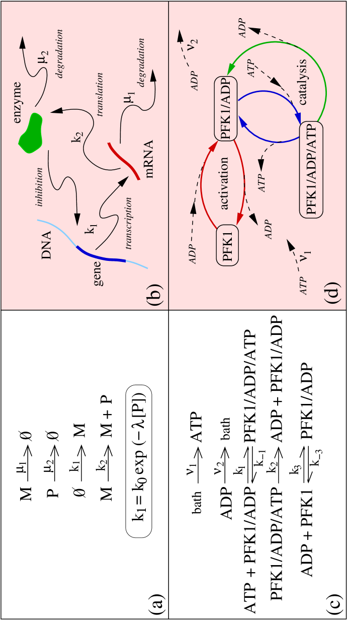
Figure 1:

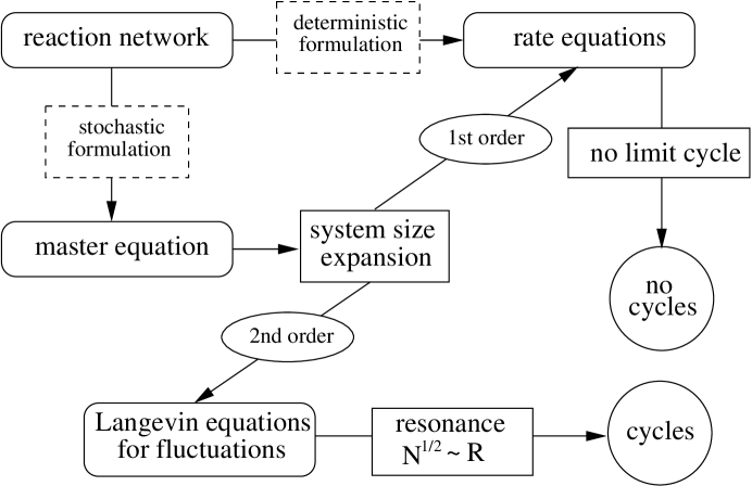
Figure 2:

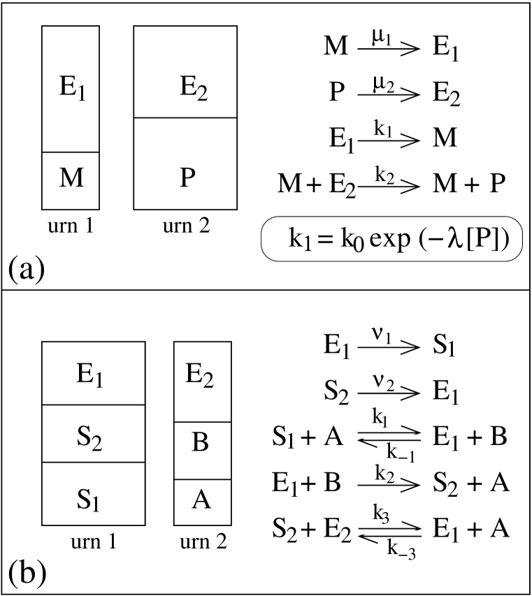
Figure 3:

Figure 4:

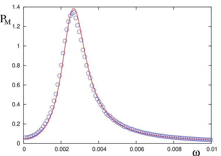
Figure 5:

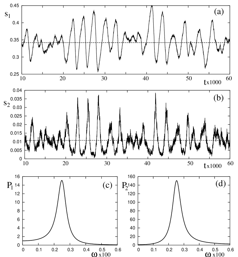
Figure 6: