Diffusion of transcription factors can drastically enhance the noise in gene expression

Abstract

We study by simulation the effect of the diffusive motion of repressor molecules on the noise in mRNA and protein levels in the case of a repressed gene. We find that spatial fluctuations due to diffusion can drastically enhance the noise in gene expression. For a fixed repressor strength, the noise due to diffusion can be minimized by increasing the number of repressors or by decreasing the rate of the open complex formation. We also show that the effect of spatial fluctuations can be well described by a two-step kinetic scheme, where formation of an encounter complex by diffusion and the subsequent association reaction are treated separately. Our results also emphasize that power spectra are a highly useful tool for studying the propagation of noise through the different stages of gene expression.

key words: gene expression, noise, systems biology, computer simulation

I Introduction

Cells process information from the outside and regulate their internal state by means of proteins and DNA that chemically and physically interact with one another. These biochemical networks are often highly stochastic, because in living cells the reactants often occur in small numbers. This is particularly important in gene expression McAdams and Arkin (1997); Elowitz et al. (2002); Ozbudak et al. (2002), where transcription factors are frequently present in copy numbers as low as tens of molecules per cell. While it is generally believed that biochemical noise can be detrimental to cell function Rao et al. (2002), it is increasingly becoming recognized that noise can also be beneficial to the organism Kaern et al. (2005). Understanding noise in gene expression is thus important for understanding cell function, and this observation has recently stimulated much theoretical and experimental work in this direction Rao et al. (2002); Kaern et al. (2005). However, the theoretical analyses usually employ the zero-dimensional chemical master equation van Kampen (2001); Gillespie (1976). This approach takes into account the discrete character of the reactants and the probabilistic nature of chemical reactions. It does assume, however, that the cell is a ‘well-stirred’ reactor, in which the particles are uniformly distributed in space at all times; the reaction rates only depend upon the global concentrations of the reactants and not upon the spatial positions of the reactant molecules. Yet, in order to react, reactants first have to move towards one another. They do so by diffusion, or, in the case of eukaryotes, by a combination of diffusion and active transport. Both processes are stochastic in nature and this could contribute to the noise in the network. Here, we study by computer simulation the expression of a single gene that is under the control of a repressor $R$ in a spatially-resolved model. We find that at low repressor concentration, i.e. $[R]<50{\rm nM}$, the noise in gene expression is dominated by the noise arising from the diffusive motion of the repressor molecules. Our results thus show that spatial fluctuations of the reactants can be an important source of noise in biochemical networks.

Our analysis reveals that in gene expression significant fluctuations occur on both small and large length and time scales. As expected from earlier work Swain et al. (2002); Paulsson (2004); Rosenfeld et al. (2005), the fluctuations on long time scales are predominantly due to protein degradation; we assume that proteins are degraded by dilution, which means that the relaxation rate of this process is on the order of an hour. Our results, however, also elucidate an important process on much smaller length and time scales. It is associated with the competition between repressor and RNA polymerase (RNAP) for binding to the promoter. When a repressor molecule dissociates from the DNA, it can rebind very rapidly, i.e. on a time scale of microseconds, or less. This rebinding time is so short that when a repressor molecule has just dissociated, the probability that a RNAP will bind before the repressor molecule rebinds, is very small. As a result, a repressor molecule will on average rebind many times, before it eventually diffuses away from the promoter and a RNAP molecule, or another repressor molecule, can bind to the promoter. This process of rapid rebindings decreases the effective dissociation rate, and this increases the noise in gene expression.

Clearly, fluctuations in gene expression span orders of magnitude in length and time scales. This means that the simulation technique should be sufficiently detailed to resolve the events at small length and time scales, yet also efficient enough to access the long length and time scales. Recently, several simulation techniques have been developed for the stochastic modeling of reaction-diffusion systems Elf and Ehrenberg (2004); Ander et al. (2004). These techniques, however, do not satisfy both criteria: they either describe the system in a coarse-grained way, i.e. on the level of local concentrations rather than single particles Elf and Ehrenberg (2004); Ander et al. (2004), or are too slow to accurately model the dynamics on the long time scales Andrews and Bray (2004). Our simulations have been made possible via the use of our recently developed Green’s Function Reaction Dynamics (GFRD) algorithm van Zon and ten Wolde (2005a); van Zon and ten Wolde (2005b). GFRD is an event driven algorithm that uses Green’s functions to combine in one step the propagation of the particles in space with the reactions between them. The event-driven nature of the algorithm makes it particularly useful for problems, such as gene expression, in which the events are distributed over a wide range of length and time scales: the algorithm takes small steps when the reactants are close to each other – such as when a repressor molecule has just dissociated from the DNA – while it takes large jumps in time and space when the molecules are far apart from each other – like when the repressor molecule has eventually diffused away from the promoter. The event-driven nature of GFRD makes it orders of magnitude more efficient than brute-force particle-based algorithms van Zon and ten Wolde (2005b) and this has allowed us to simulate gene expression on the relevant biological time scales of hours.

Several publications M. S. H. Ko (1991); Kepler and Elston (2001); Karmakar and Bose (2004); Pirone and Elston (2004); Simpson et al. (2004); Bialek and Setayeshgar (2005); Hornos et al. (2005) have discussed the effect of fluctuations in the binding of transcription factors to their site on the DNA (called operator) on the noise in gene expression. Most of these models are relatively simple, ignoring, for instance, production of mRNA Kepler and Elston (2001); Karmakar and Bose (2004); Pirone and Elston (2004); Hornos et al. (2005). Moreover all these studies, with the exception of Metzler (2001); Bialek and Setayeshgar (2005), ignore the role of the spatial fluctuations of the transcription factors. Our aim is to study gene expression in a biologically meaningful model. We have therefore constructed a rather detailed model, although we will also use minimal models that can be studied analytically, in order to interpret the simulation results. The full model, which is described in the next section, contains the diffusive motion of repressor molecules, open complex formation, promoter clearance, transcription elongation and translation Record et al. (1996).

In section IV, we discuss the simulation results for both the noise in mRNA and protein level. The results reveal that for $[R]<50{\rm nM}$, the noise in the spatially-resolved model can be more than five times larger than the noise in the well-stirred model. We also show that a cell could minimize the effect of spatial fluctuations, either by tuning the open complex formation rate or by changing the number of repressors and their affinity for the binding site on the DNA. In section V, we elucidate the origin of the enhanced noise in the spatially resolved model. In the subsequent section, we show that in the model employed here the effect of spatial fluctuations can be quantitatively described by a well-stirred model in which the reaction rates for repressor binding and unbinding are appropriately renormalized; however, as we discuss in the last section, we expect that in a more refined model the effect of diffusion will be more complex, impeding such a simplified description. In section VII, we discuss how the operator state fluctuations propagate through the different stages of gene expression using power spectra for the operator state, elongation complex, mRNA and protein. The results show that these power spectra are highly useful for unraveling the dynamics of gene expression. We hope that this stimulates experimentalists to measure power spectra of not only mRNA and protein levels Austin et al. (2006), but also of the dynamics of transcription initiation and elongation using e.g. magnetic tweezers Revyakin et al. (2004). As we argue in the last section, such experiments should make it possible to determine the importance of spatial fluctuations for the noise in gene expression.

II Model

II.1 Diffusive motion of repressors

We explicitly simulate the diffusive motion of the repressor molecules in space. However, since the experiments of Riggs et al. Riggs et al. (1970) and the theoretical work of Berg, Winter, and Von Hippel Berg et al. (1981), it is well known that proteins could find their target sites via a combination of 1D sliding along the DNA and 3D diffusion through the cytoplasm – “hopping” or “jumping” from one site on the DNA to another. This mechanism could speed up the search process and make it faster than the rate at which particles find their target by free 3D diffusion; this rate is given by $k=4\pi\sigma D_{3}[R]$, where $\sigma$ is the cross section, which is on the order of a protein diameter or DNA diameter, $D_{3}$ is the diffusion constant of the protein in the cytoplasm, and $[R]$ is the concentration of the (repressor) protein. However, while it is clear that the mechanism of 3D diffusion and 1D sliding could potentially speed up the search process, whether this mechanism in living cells indeed drastically reduces the search time is still under debate Halford and Marko (2004). In this context, it is instructive to discuss the two main results of recent studies on this topic Gerland et al. (2002); Coppey et al. (2004); Slutsky and Mirny (2004); Halford and Marko (2004); Klenin et al. (2006); Hu et al. (2006). The first is that the mean search time $\tau$ is given by Hu et al. (2006)

$$\tau\sim\frac{L}{\lambda}\left[\frac{\lambda^{2}}{D_{1}}+\frac{r^{2}}{D_{3}}\right],$$ (1)

where $L$ is the total length of the DNA, $\lambda$ is the average distance over which the protein slides along the DNA before it dissociates, $D_{1}$ is the diffusion constant for sliding, $r$ is the typical mesh size in the nucleoid, and $D_{3}$ is the diffusion constant in the cytoplasm. This formula has a clear interpretation Hu et al. (2006): $\lambda^{2}/D_{1}$ is the sliding time, $r^{2}/D_{3}$ is the time spent on 3D diffusion, the sum of these terms is thus the time to perform one round of sliding and diffusion, and $L/\lambda$ is the total number of rounds needed to find the target. The other principal result is that the search time is minimized when the sliding distance $\lambda$ is

$$\lambda=\sqrt{\frac{D_{1}}{D_{3}}}r.$$ (2)

Under these conditions, a protein spends equal amounts of time on 3D diffusion and 1D sliding (a protein is thus half the time bound to the DNA). Eq. 2 is a useful result, because it shows that the average sliding distance $\lambda$ depends upon the ratio of diffusion constants and on the typical mesh size in the nucleoid. If we now assume that $D_{1}$ and $D_{3}$ are equal (which is not obvious given that proteins bind relatively strongly to DNA – $D_{1}$ could thus very well be much smaller than $D_{3}$) and if we take the mesh size to be given by $r\sim\sqrt{v/L}$ Hu et al. (2006), where $v\approx 1\mu{\rm m}^{3}$ is the volume of an Escherichia coli cell and $L\approx 10^{3}\mu{\rm m}$, we find that $\lambda\approx 10{\rm nm}$ (30 bp). This corresponds to the typical diameter of a protein or DNA double helix and is thus not very large. Interestingly, recent experiments seem to confirm this: experiments from Halford et al. on restriction enzymes (EcoRV and BbcCI) with a series of DNA substrates with two target sites and varying lengths of DNA between the two sites, suggest that under the in vivo conditions, sliding is indeed limited to relatively short distances, i.e. to distances less than 50 bp ($\approx 16{\rm nm}$) Stanford et al. (2000); Gowers et al. (2005).

Now, it should be realized that on length scales beyond the sliding length, the motion is essentially 3D diffusion: the sliding/hopping mechanism corresponds to 3D diffusion with a jump distance given by the sliding distance Gerland et al. (2002). Moreover, since the sliding distance is only on the order of a particle diameter, as discussed above, we have therefore decided to model the motion of the repressor molecules as 3D diffusion. But it should be remembered that on length scales smaller than $10-30{\rm nm}$, this approach is not correct. We discuss the implications of this for our results in the Discussion section.

II.2 Transcription and Translation

Most repressors bind to a site that (partially) overlaps with the core promoter – the binding site of the RNA polymerase (RNAP). When a repressor molecule is bound to its operator site, it prevents RNAP from binding to the promoter, thereby switching off gene expression. Only in the absence of a repressor on the operator site, can RNAP bind to the promoter and initiate transcription and translation, ultimately resulting in the production of a protein. We model this by the following reaction network:

$$O+R \overset{k_{\rm fR}}{\underset{k_{\rm bR}}{\rightleftarrows}} OR$$ (3)

$$O \overset{k_{\rm fRp}}{\underset{k_{\rm bRp}}{\rightleftarrows}} ORp$$ (4)

$$ORp \underset{k_{\text{OC}}}{\rightarrow} ORp^{*}$$ (5)

$$ORp^{*} \underset{t_{\text{clear}}}{\rightarrow} T+O$$ (6)

$$T \underset{t_{\text{elon}}}{\rightarrow} M$$ (7)

$$M \underset{k_{\text{dm}}}{\rightarrow} \varnothing$$ (8)

$$M \underset{k_{\text{ribo}}}{\rightarrow} M+M_{\rm ribo}$$ (9)

$$M_{\rm ribo} \underset{t_{\text{trans}}}{\rightarrow} P$$ (10)

$$P \underset{k_{\text{dp}}}{\rightarrow} \varnothing$$ (11)

Eqs. 3 and 4 describe the competition between the binding of the repressor $R$ and the RNAP molecules $Rp$ to the promoter ($O$ is the operator site). In our simulation we fix the binding site $O$ in the center of a container with volume $V=1\mu{\rm m}^{3}$, comparable to the volume of a single E. coli cell. We simulate both the operator site $O$ and the repressor molecules as spherical particles with diameter $\sigma=10$nm. The operator site $O$ is surrounded by $N_{R}$ repressor molecules that move by free 3D diffusion (see previous section) with an effective diffusion constant $D=1\mu{\rm m}^{2}s^{-1}$, as has been reported for proteins of a similar size Elowitz et al. (1999). The intrinsic forward rate $k_{\text{fR}}=6\cdot 10^{9}M^{-1}s^{-1}$ for the repressor particles $R$ at contact is estimated from the Maxwell-Boltzmann distribution van Zon and ten Wolde (2005a). The backward rate $k_{\text{bR}}$ depends on the interaction between the DNA binding site of the repressor and the operator site on the DNA and varies greatly between different operons, with stronger repressors having a lower $k_{\text{bR}}$. In our simulations, we vary $k_{\text{bR}}$ between $1-0.01\ s^{-1}$, as discussed in more detail below. The concentration of RNAP is much higher than that of the repressor Bremer et al. (2003). Because of this we treat the RNAP as distributed homogeneously within the cell and we do not to take diffusion of RNAP into account explicitly. Instead, RNAP associates with the promoter with a diffusion-limited rate $k_{\text{fRp}}=4\pi\sigma D[Rp]$. In our simulations, the concentration of free RNAP is $[Rp]=0.5\mu M$ Bremer et al. (2003), leading to a forward rate $k_{\text{fRp}}=38s^{-1}$. Finally, the backward rate $k_{\text{bRp}}=0.5$ is determined such that $K_{\text{eq}}=4\pi\sigma D/k_{\text{bRp}}=1.4\cdot 10^{9}M^{-1}$ McClure (1983).

Transcription initiation is described by Eqs. 5 and 6. Before productive synthesis of RNA occurs, first the RNAP in the RNAP-promoter complex $ORp$ unwinds approximately one turn of the promoter DNA to form the open complex $ORp^{*}$. The open complex formation rate $k_{\text{OC}}$ has been measured to be on the order of $0.3-3s^{-1}$ Revyakin et al. (2004). We approximate open complex formation as an irreversible reaction. Some experiments find this step to be weakly reversible Revyakin et al. (2004). However, adding a backward reaction to the model did not change the dynamics of the system in a qualitative way, as long as the backward rate is smaller than $k_{\text{OC}}$, which is in agreement with experimental results. After open complex formation, RNAP must first escape the promoter region before another RNAP or repressor can bind. Since elongation occurs at a rate of $50-100$ nucleotides per second and between $30-60$ nucleotides must be cleared by RNAP before the promoter is accessible, a waiting time of $t_{\text{clear}}=1s$ is required before another binding can occur. Since promoter clearance consists of many individual elongation events that obey Poisson statistics individually, we model the step as one with a fixed time delay $t_{\text{clear}}$, not as a Poisson process with rate $1/t_{\text{clear}}$.

Eqs. 7-11 describe the dynamics of mRNA and protein numbers. After clearing the promoter region, RNAP starts elongation of the transcript $T$. As for clearance, the elongation step is modeled as a process with a fixed time delay $t_{\text{elon}}=30s$, corresponding to an elongation rate of $50-100$ nucleotides per second and a $1500$ bp gene. When a mRNA $M$ is formed, it can degrade with a rate $k_{\text{dm}}$. Here, the mRNA degradation rate is determined by fixing the average mRNA concentration in the unrepressed state, as described below. Furthermore, a mRNA molecule can form a mRNA-ribosome complex $M_{\rm ribo}$ and start translation. We assume that $b=5$ proteins are produced on average from a single mRNA molecule Ozbudak et al. (2002), so that the start of translation occurs at a rate $k_{\text{ribo}}=b\ k_{\text{dm}}$. After a fixed time delay $t_{\text{trans}}=30s$ a protein $P$ is produced. The mRNA is available for ribosome binding immediately after the start of translation. Due to the delay in protein production, $M$ can start to be degraded, while the mRNA-ribosome complex $M_{\rm ribo}$ is still present; $M$ thus represents the mRNA leader region rather than the entire mRNA molecule. Finally, the protein $P$ degrades at a rate $k_{\text{dp}}$, which is determined by the requirement that the average protein concentration in the unrepressed state has a desired value, as we describe now.

We vary the free parameters in the reaction network described in Eqs. 3-11 – $N_{R}$, $k_{\rm bR}$, $k_{\rm dm}$, $k_{\rm dp}$ – in the following way: first, we choose the concentration of mRNA and protein in the absence of repressor molecules. In this case, tuning of the concentrations is most straightforward by adjustment of the mRNA and protein decay rates $k_{\text{dm}}$ and $k_{\text{dp}}$. For the above reaction network one can show that the average mRNA number $N_{M}$and protein number $N_{P}$ is given by

$$N_{M} = \frac{K_{4}K_{1}V}{K_{2}N_{R}+V(1+K_{1}(1+K_{3}))},$$ (12)

$$N_{P} = K_{5}N_{M},$$ (13)

where $K_{1}=k_{\text{fRp}}/(k_{bRp}+k_{\text{OC}})$, $K_{2}=k_{\text{fR}}/k_{\text{bR}}$, $K_{3}=k_{\text{OC}}t_{\text{clear}}$, $K_{4}=k_{\text{OC}}/k_{\text{dm}}$ and $K_{5}=k_{\text{ribo}}/k_{\text{dp}}$ are equilibrium constants, $V$ is the volume of the cell and $N_{R}$ is the total number of repressors. The unrepressed state corresponds to $N_{R}=0$. In our simulations, we fix the mRNA and protein numbers in the unrepressed state at $N_{M}=50$ and $N_{P}=2\cdot 10^{5}$. The mRNA and protein decay rates then follow straightforwardly from Eqs. 12 and 13: the mRNA degradation rate is $k_{\rm dm}=0.019{\rm s}^{-1}$ Kushner (1996) and the protein degradation rate is $k_{\rm dp}=2.4\times 10^{-4}{\rm s}^{-1}$; the latter corresponds to protein degradation by dilution with a cell cycle time of around 1h.

Next, we determine by what factor these concentrations should decrease in the repressed state. This can be done by changing the number of repressors $N_{R}$ and the repressor backward rate $k_{\text{bR}}$. We define the repression level $f$ as the transcription initiation rate in the absence of repressors, divided by the initiation rate in the repressed state Vilar and Leibler (2003). For a repression level $f$, the concentration of mRNA and proteins in the repressed state is a fraction $1/f$ of the concentration in the unrepressed state and it follows that

$$\frac{N_{R}}{k_{\text{bR}}}=(f-1)\frac{V(1+K_{1}(1+K_{3}))}{k_{\text{fR}}}.$$ (14)

Thus, a fixed repression level $f$ does not specify a unique combination of $N_{R}$ and $k_{\text{bR}}$: increasing the number of repressors twofold, while also increasing the repressor backward rate by the same factor, gives the same repression level. This means that the cell can control mRNA and protein levels in the repressed state either by having a large number of repressors that stay on the DNA for a short time or by having a small number of repressors, possibly even one, that stay on the DNA for a long time. Even though it is conceivable that the latter is preferable for economic reasons, there is no difference between the two extremes in terms of the average gene expression. In our simulations, we vary $N_{R}$ and $k_{\rm bR}$, but use a fixed repression level $f=100$. Consequently, in the repressed state, on average $N_{\text{M}}=0.5$ and $N_{\text{P}}=200$.

III Simulation Technique

We simulate the above reaction network using Green’s Function Reaction Dynamics (GFRD) van Zon and ten Wolde (2005a); van Zon and ten Wolde (2005b). As discussed above, only the operator site $O$ and the repressor particles $R$ are simulated in space. All other reactions are assumed to occur homogeneously within the cell and are simulated according to the well-stirred model Gillespie (1977) or with fixed time delays for reaction steps involving elongation. A few modifications with respect to the algorithm described in van Zon and ten Wolde (2005a); van Zon and ten Wolde (2005b) are implemented to improve simulation speed. First, we neglect excluded volume interactions between repressor particles mutually, as the concentration of repressor is very low. This means that the only potential reaction pairs we consider are operator-repressor pairs. Secondly, we use periodic boundary conditions instead of a reflecting boundary, which leads to a larger average time step. As the operator site $O$ is both small compared to the volume of the cell and is far removed from the cell boundary, this has no effect on the dynamics of the system. Finally, as the repressor backward rate $k_{\text{bR}}$ is rather small, the operator site can be occupied by a repressor for a time long compared to the average simulation time step. If the repressor is bound to the operator site longer than a time $L^{2}/6D$, where $L$ is the length of the sides of our container, the other repressor molecules diffuse on average from one side of the box to the other. Consequently, when the repressor eventually dissociates from the operator site, the other repressor molecules have lost all memory of their positions at the time of repressor binding. Here, when a repressor will dissociate after a time longer than $L^{2}/6D$, we do not propagate the other repressors with GFRD, but we only update the master equation and fixed delay reactions. We update the positions of the free repressors at the moment that the operator site becomes accessible again, by assigning each free repressor molecule a random position in the container; the dissociated repressor is put at contact with the operator site. We see no noticeable difference between this scheme and results obtained by the full GFRD algorithm described in Refs. van Zon and ten Wolde (2005a); van Zon and ten Wolde (2005b).

IV Simulation results: dynamics and noise

To study the effect of spatial fluctuations on the repression of genes, we simulate the reaction network described in Eqs. 3-11 both by GFRD, thus explicitly taking into account the diffusive motion of the repressor particles, and according to the well-stirred model, where the repressor particles are assumed to be homogeneously distributed in space and the dynamics depends only on the concentration of repressor. In Fig. 1 we show the behavior of mRNA and protein numbers for a system with open complex formation rate $k_{\text{OC}}=30s^{-1}$ and with varying numbers of repressors $N_{R}$. We keep the repression factor fixed at $f=100$ so that with increasing $N_{R}$ the repressor backward rate $k_{\text{bR}}$ is also increased, i.e. repressor particles are bound to the DNA for a shorter time.

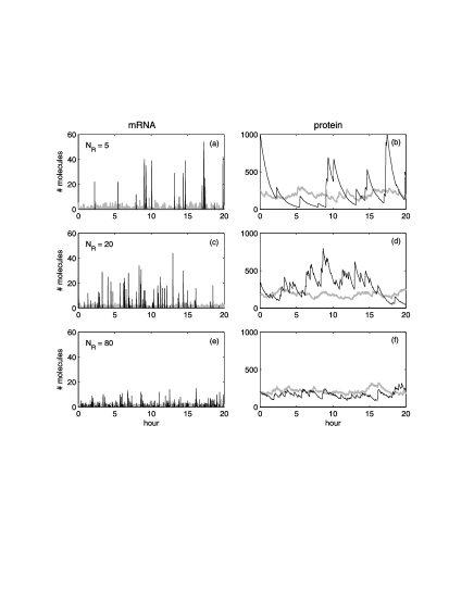
Figure 1: Dynamics of mRNA and protein numbers in the repressed state for different number of repressors $N_{R}$. The number of mRNA and protein molecules is shown for simulations with GFRD (black line) and according to the master equation (gray line). In the GFRD simulation, diffusion of repressor particles is explicitly included. (a) and (b) $N_{R}=5$. (c) and (d) $N_{R}=20$. (e) and (f) $N_{R}=80$. In general, there is a dramatic difference in dynamics due to the spatial fluctuations of the repressor molecules. This difference becomes more pronounced as the number of repressors decreases. However, we find that in all cases $\langle N_{\text{M}}\rangle=0.5$ and $\langle N_{P}\rangle=200$, on average.

It is clear from Fig. 1 that there is a dramatic difference between the behavior of mRNA and protein numbers between the GFRD simulation and the well-stirred model. When spatial fluctuations of the repressor molecules are included, mRNA is no longer produced in a continuous fashion, but instead in sharp, discontinuous bursts during which the mRNA level can reach levels comparing to those of the unrepressed state. These bursts in mRNA production consequently lead to peaks in protein number. As the protein decay rate is much lower than that of mRNA, these peaks are followed by periods of exponential decay over the course of hours. Due to these fluctuations, protein numbers often reach levels of around $5-10\%$ of the protein levels in the unrepressed state. In contrast, in the absence of repressor diffusion, the fluctuations around the average protein number are much lower. For both cases, however, the average behavior is identical: even though the dynamics is very different, we always find that on average $\langle N_{\text{mRNA}}\rangle=0.5$ and $\langle N_{P}\rangle=200$. Also, in all cases the fluctuations in mRNA number are larger than those in protein number. This means that the translation step functions as a low-pass filter to the repressor signal.

When we increase the number of repressors $N_{R}$ and change $k_{\text{bR}}$ in such a way that the repression level $f$ remains constant, we find that both for GFRD and the well-stirred model the fluctuations in mRNA and protein number decrease. In the absence of spatial fluctuations this effect is minor, but for GFRD this decrease is sharp: for large number of repressors, the burst in mRNA become both weaker and more frequent. This in turn leads to smaller peaks and shorter periods of exponential decay in protein numbers. In fact, as $N_{R}$ is increased both approaches converge to the same behavior. At around $N_{R}\approx 100$, the dynamics of the protein number is similar for the well-stirred model and the spatially resolved model. The same happens for mRNA number when $N_{R}\approx 500$.

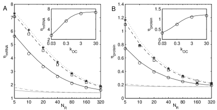
Figure 2: Noise in (a) mRNA number and (b) protein number as a function of the number of repressors $N_{R}$ and for constant repression factor $f=100$. Data obtained by GFRD simulation is shown for $k_{\rm OC}=0.3(\circ),3(\Box)$ and $30(*)s^{-1}$. Noise levels for the well-stirred model are shown as grey lines and those for the well-stirred model with reaction rates renormalized according to Eqs. 16 and 17 are shown as black lines, both for $k_{\rm OC}=0.3$ (solid lines), $3$ (dashed lines) and $30$ (dotted lines) $s^{-1}$. Only when the reaction rates are properly renormalized does the noise in the well-stirred model agree well with the noise in the GFRD simulations, which include the effect of diffusion. (Insets) Noise levels as a function of $k_{\rm OC}$. Symbols indicate results for GFRD and lines are results for the chemical master equation with renormalized reaction rates.

In Fig. 2, we quantify the noise in mRNA and protein number, defined as standard deviation divided by the mean, while we change the number of repressors $N_{R}$. As we keep the amount of repression fixed at $f=100$, we simultaneously vary the backward rate $k_{\rm bR}$ according to Eq. 14. When all parameters are the same, the noise for the GFRD simulation, including the diffusive motion of the repressors, is always larger than the noise for the well-stirred model, where the diffusive motion is ignored. In both cases, the noise decreases when the number of repressors is increased and the repressor backward rate becomes larger. This is consistent with the mRNA and protein tracks shown in Fig. 1. We also investigated the effect of changing the open complex formation rate $k_{\rm OC}$. In nature, this rate can be tuned by changing the base pair composition of the promoter region on the DNA. When we change $k_{OC}$, we change the mRNA decay rate $k_{\rm dm}$ so that the average mRNA and protein concentrations remain unchanged (see section II.2). We find that when $k_{\rm OC}$ is lowered, the fluctuations in mRNA and protein levels are sharply reduced. When $k_{\rm OC}$ is much larger than the RNAP backward rate $k_{\rm bRp}=0.5s^{-1}$, almost every RNAP binding to the promoter DNA will result in transcription of a mRNA. For $k_{\rm OC}$ smaller than $k_{\rm bRp}$, RNAP binding will lead to transcription only infrequently. As a consequence, the operator filters out part of the fluctuations in RNAP binding due to the diffusive motion of the repressor particles, leading to the decrease in noise observed in Fig. 2. This shows that the open complex formation rate plays a considerable role in controlling noise in gene expression.

V Simulations results: operator binding

To understand how the diffusive motion of repressor molecules leads to increased fluctuations in mRNA and protein numbers, it is useful to look in some detail at the dynamics of repressor-DNA binding. In figure 3A, we show the $OR$ bias for both GFRD and the well-stirred model. The $OR$ bias is a moving time average over $OR(t)$ with a $50s$ time window and should be interpreted as the fraction of time the operator site was bound by repressor particles over the last $50$ seconds. The results we show here are for $N_{R}=5$ repressors and a repression factor $f=2$. At this repression factor, $k_{\text{bR}}$ is such that the repressor molecules are bound to the operator only fifty percent of the time, making it easier to visualize the operator dynamics than in the case of $f=100$ as used above.

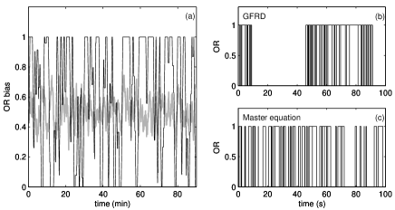
Figure 3: Dynamics of repressor binding for a repression factor of $f=2$ and $N_{R}=5$. (a) The $OR$-bias for GFRD (black line) and the well-stirred model (gray line). The $OR$-bias is defined as the fraction of time a repressor is bound to the operator site in the last $50$ seconds. When the diffusive motion of repressor molecules is included (black line), the $OR$-bias switches between periods where repressors are continuously bound to or absent from the DNA for long times. (b) and (c) Time trace of the occupancy of the operator site by repressor molecules. When $OR=1$ a repressor is bound to the operator site and $OR=0$ indicates either a free operator site or one with RNAP bound. For the GFRD simulations, an initial binding is followed by several rapid rebindings, whereas for the well-stirred model binding and rebinding is much more unstructured. Note that here, for reasons of clarity, $f=2$ instead of $f=100$ as used in the text and Figs. 1 and 2.

The $OR$ bias for the well-stirred model fluctuates around the average value $\langle OR\rangle=0.5$, indicating that on the timescale of $50s$ several binding and unbinding events occur, in agreement with $k_{\text{bR}}=1.26s^{-1}$ for $f=2$. On the other hand, when including spatial fluctuations, the $OR$ bias switches between periods in which repressors are bound to the DNA continuously and periods in which the repressors are virtually absent, both on timescales much longer than the $50s$ time window. How is it possible that repressors are bound to the operator site for times much longer than the timescale set by the dissociation rate from the DNA? The answer to that question can be found in Figs. 3B and C, where a time trace is shown of the operator occupancy by the repressor for both GFRD and the well-stirred model. The time trace for the simulation of the well-stirred model in Fig. 3C shows a familiar picture: binding and dissociation of the repressor from the operator occurs irregularly, the time between events given by Poisson distributions. The time trace for GFRD in Fig. 3B looks rather different. Here, in general a dissociation event is followed by a rebinding very rapidly. Only occasionally does a dissociation result in the operator being unbound by repressors for a longer time. When this happens, repressors stay away from the operator for a time much longer than the typical time separating binding events in Fig. 3C. These series of rapid rebindings followed by periods of prolonged absence from the operator result in the aberrant $OR$ bias shown in Fig. 3A.

The occurrence of rapid rebindings is intimately related to the nature of diffusion. When diffusion and the positions of the reactants are ignored all dynamics is based only on the average concentration of the reactants. As a consequence, when in this approach a repressor dissociates from the operator site, the probability of rebinding depends only on the concentration of repressor in the cell. On the level of actual positions of the reactants, this amounts to placing the repressor at a random position in the container. The situation is very different for the GFRD approach, where the positions of the reactants are taken into account. After a dissociation from the operator site, the repressor particle is placed at contact with the operator site. Because of the close proximity of the repressor to its binding site, it has a high probability of rapidly rebinding to, and only a small probability of diffusing away from, the binding site. At the same time, when the repressor eventually diffuses away from the operator site, the probability that the same, or more likely, another repressor diffuses to and binds the operator site is much smaller than the probability of binding in the well-stirred model, as will be shown quantitatively in Sec. VI. This results in the behavior observed in Fig. 3B.

It can now be understood that the bursts in mRNA production correspond to the prolonged absence of repressor from the operator site compared to the well-stirred model. Especially for low repressor concentrations, these periods of absence can be long enough that the concentration of mRNA reaches values comparable to those in the unrepressed state for brief periods of time. When a repressor binds to the operator site, due to the rapid rebindings it will remain bound effectively for a time much longer than the mRNA lifetime, leading to long periods where mRNA is absent in the cell. This shows that under these conditions spatial fluctuations and not stochastic chemical kinetics are the dominant contribution to the noise in mRNA and protein numbers in the repressed state.

VI Two-step kinetic scheme

In this section we investigate to what extent the effect of diffusion on the repressor dynamics can be modeled by the two-step kinetic scheme M. Eigen (1974); D. Shoup and A. Szabo (1982):

$$O+R\overset{k_{+}}{\underset{k_{-}}{\rightleftarrows}}O\cdots R\overset{k_{a}}{\underset{k_{d}}{\rightleftarrows}}OR.\\$$ (15)

The first step in Eq. 15 describes the diffusion of repressor to the operator site resulting in the encounter complex $O\cdots R$, with the rates $k_{+}$ and $k_{-}$ depending on the diffusion coefficient $D$ and the size of the particles. The next step describes the subsequent binding of repressor to the DNA. In this case the rates are related to the microscopic rates defined in Eq. 3. When the encounter complex is assumed to be in steady state, the two-step kinetic scheme can be mapped onto the reaction described in Eq. 3, but with effective rate constants $k^{\prime}_{fR}=k_{+}k_{a}/(k_{-}+k_{a})$ and $k^{\prime}_{bR}=k_{-}k_{d}/(k_{-}+k_{a})$ M. Eigen (1974). The two-step kinetic scheme should yield the same average concentrations as the scheme in Eq. 3, so that the equilibrium constant $K=k_{a}/k_{d}=k^{\prime}_{fR}/k^{\prime}_{bR}=k_{fR}/k_{bR}$, where $k_{\rm fR}$ and $k_{\rm bR}$ are the reaction rates defined in Eq. 3.

It is possible to express the effective rate constants $k^{\prime}_{\rm fR}$ and $k^{\prime}_{\rm bR}$ in terms of the microscopic rate constants $k_{\rm fR}$ and $k_{\rm bR}$. For the setup used here, where a single operator O is surrounded by a homogeneous distribution of repressor R, the rate $k_{+}$ follows from the solution of the steady state diffusion equation with a reactive boundary condition with rate $k=k_{a}$ at contact M. Smoluchowski (1917); D. Shoup and A. Szabo (1982) and is given by the diffusion-limited reaction rate $k_{D}=4\pi\sigma D$. The rates $k_{-}$ and $k_{a}$ depend on the exact definition of the encounter complex $O\cdots R$. It is natural to identify the rate $k_{d}$ with the intrinsic dissociation rate $k_{bR}$, thus $k_{d}=k_{bR}$. From these expressions for $k_{+}$ and $k_{d}$ and the requirement that the equilibrium constant should remain unchanged, one finds that $k_{a}/k_{-}=k_{fR}/k_{D}$. Using this result one obtains $k^{\prime}_{fR}=k_{D}k_{fR}/(k_{D}+k_{fR})$ and $k^{\prime}_{bR}=k_{D}k_{bR}/(k_{D}+k_{fR})$.

These renormalized rate constants have a clear interpretation. For the effective forward rate it follows, for instance, that: $1/k^{\prime}_{fR}=1/k_{D}+1/k_{fR}$: that is, on average, the time required for repressor binding is given by the time needed to diffuse towards the operator plus the time for a reaction to occur when the repressor is in contact with the operator site D. Shoup and A. Szabo (1982). The effective backward rate has a similar interpretation. The probability that after dissociation the repressor diffuses away from the operator site and never returns is given by $S_{\rm irr}(t\rightarrow\infty|\sigma)$, where $S_{\rm irr}(t,r_{0})$ is the irreversible survival probability for two reacting particles Kim and Shin (1999). Using that $S_{\rm irr}(t\rightarrow\infty|\sigma)=k_{D}/(k_{fR}+k_{D})$, the expression for $k^{\prime}_{bR}$ can be written as $k^{\prime}_{bR}=k_{bR}S_{\rm irr}(t\rightarrow\infty|\sigma)$: that is, the effective dissociation rate is the microscopic dissociation rate multiplied by the probability that after dissociation the repressor escapes from the operator site D. Shoup and A. Szabo (1982).

For diffusion limited reactions, such as the reaction considered here, we have that $k_{fR}\gg k_{D}$. Now, the renormalized rate constants reduce to:

$$k^{\prime}_{fR} = k_{D},$$ (16)

$$k^{\prime}_{bR} = k_{D}k_{bR}/k_{fR}.$$ (17)

In Fig. 2, we compare the noise profiles for the GFRD algorithm with those obtained by a simulation of the well-stirred model, where instead of the microscopic rates $k_{fR}$ and $k_{fB}$ we use the renormalized rates from Eqs. 16 and 17. Surprisingly, we find complete agreement. One of the main reasons why this is unexpected, is that for the master equation the time between events is Poisson-distributed, whereas after a dissociation the time to the next rebinding is distributed according to a power-law distribution when diffusion is taken into account Kim and Shin (1999). The reason that this power-law behavior of rebinding times is not of influence on the noise profile, is that the time scale of rapid rebinding is much smaller than any of the other relevant time scales in the network. Specifically, rebinding times are so short that the probability that a RNAP will bind before a rebinding is negligible. As a consequence, the transcription network is not at all influenced by the brief period the operator site is accessible before rebinding: for the transcription machinery the series of consecutive rebindings, albeit distributed algebraically in time individually, is perceived as a single event. And on much longer time scales, when a repressor diffuses in from the bulk towards the operator site, the distribution of arrival times is expected to be Poissonian, because on these time scales the repressors are distributed homogeneously in the bulk.

It is possible to reinterpret the effective rate constants in Eq. 16 and 17 in the language of rapid rebindings. The probability $p$ that a rebind will occur after a dissociation from the DNA is given by $p=1-S_{\infty}$, where $S_{t}=S_{\rm irr}(t,r_{0}=\sigma)$. The probability that $n$ consecutive rebindings occur before the repressor diffuses away from the operator site is then given by $p_{n}=(1-S_{\infty})^{n}S_{\infty}$. From this follows that the average number of rebindings is $N_{RB}=(1-S_{\infty})/S_{\infty}$. Using again that $S_{\infty}=k_{D}/(k_{fR}+k_{D})$, we find that $N_{RB}=k_{fR}/k_{D}$. Combining this with Eqs. 16 and 17, we get:

$$k^{\prime}_{fR} = k_{fR}/N_{RB},$$ (18)

$$k^{\prime}_{bR} = k_{bR}/N_{RB}.$$ (19)

In words, after an initial binding the repressor spends $N_{RB}$ times longer on the DNA than expected on the basis of the microscopic backward rate, as it rebinds on average $N_{RB}$ times. Because the average occupancy should not change, the forward rate should be renormalized in the same way. In conclusion, in this model the effects of diffusion can be properly described by a well-stirred model when the reaction rates are renormalized by the average number of rebindings.

VII Power Spectra

In this section, we study how the noise due to the stochastic dynamics of the repressor molecules propagates through the different steps of gene expression for both the spatially resolved model and the well-stirred model. This analysis will also provide further insight into why the well-stirred model with renormalized rate constants for the (un)binding of the repressor molecules works so well.

In biochemical networks, the noise in the output signal depends upon the noise in the biochemical reactions that constitute the network, the so-called intrinsic noise, and on the noise in the input signal, called extrinsic noise Elowitz et al. (2002); Pedraza and van Oudenaarden (2005); Detwiler et al. (2000); Paulsson (2004); Shibata and Fujimoto (2005); Tănase-Nicola et al. (2005). In our case, the output signal is the protein concentration, while the input signal is provided by the repressor concentration. The intrinsic noise arises from the biochemical reactions that constitute the transcription and translation steps. Moreover, we consider the noise in the protein concentration that is due to the (un)binding of the RNAP to (from) the DNA to be part of the intrinsic noise. The extrinsic noise is provided by the fluctuations in the binding of the repressor to the operator, i.e. in the state OR. Since the total repressor concentration, $[R_{\rm T}]=[R]+[OR]$, is constant, the extrinsic noise is also given by the fluctuations in the concentration of unbound repressor.

The noise properties of biochemical networks are most clearly elucidated via the power spectra of the time traces of the copy numbers of the components. Recently, we have shown that if the fluctuations in the input signal are uncorrelated with the noise in the biochemical reactions that constitute the processing network, the power spectrum of the output signal is given by Tănase-Nicola et al. (2005)

$$S_{\rm P}(\omega)=S_{\rm in}(\omega)+g(\omega)S_{\rm ex}(\omega).$$ (20)

Here, $S_{\rm P}(\omega)$ is the power spectrum of the output signal, the protein concentration. The spectrum $S_{\rm in}(\omega)$ denotes the intrinsic noise of the processing network; it is defined as the noise in the output signal in the absence of noise in the input signal. Here, the intrinsic noise is due to the biochemical reactions of transcription and translation. The spectrum $S_{\rm ex}(\omega)$ is the power spectrum of the input signal, which, in this case, is given by the noise in the concentration of unbound repressor: $S_{\rm ex}(\omega)=S_{\rm R}(\omega)$; because the total repressor concentration is constant this power spectrum is also directly related to that of the repressor-bound state of the operator, $S_{\rm OR}(\omega)$. The function $g(\omega)$ is a transfer function, which indicates how fluctuations in the input signal are transmitted towards the output signal. If the extrinsic noise is uncorrelated with the intrinsic noise, then $g(\omega)$ is an intrinsic quantity that only depends upon properties of the processing network, and not upon properties of the incoming signal Tănase-Nicola et al. (2005). However, for the network studied here, the noise in the input signal is not uncorrelated with the intrinsic noise Tănase-Nicola et al. (2005). As we have shown recently, this means that Eq. 20 is not strictly valid Tănase-Nicola et al. (2005); the extrinsic contribution to the power spectrum of the output signal can no longer be factorized into a function that only depends upon intrinsic properties of the network, $g(\omega)$, and one that only depends upon the input signal, $S_{\rm ex}(\omega)$. This relation is nevertheless highly instructive. Indeed, Eq. 20 could be interpreted as a heuristic definition of the transfer function $g(\omega)$.

The diffusive motion of the repressor molecules impede an analytical evaluation of the power spectrum for the extrinsic noise. Moreover, while power spectra can be calculated analytically for linear reaction networks Warren et al. (2005), the delays in transcription resulting from promoter clearance and elongation, preclude the derivation of an analytical expression for the power spectrum of the intrinsic noise. We have therefore obtained the power spectra $S_{\rm P}(\omega)$, $S_{\rm ex}(\omega)$, and $S_{\rm in}(\omega)$, directly from the time traces of the copy numbers. The power spectrum of a component ${\rm X}$ is given by $S_{\rm X}(\omega)=\langle|\tilde{X}(\omega)|^{2}\rangle$, where $\tilde{X}(\omega)$ is the Fourier Transform of the concentration $X(t)$ of component ${\rm X}$. Conventional FFT algorithms are not convenient, because our signals vary over a wide range of time scales. We therefore adopted a novel and efficient procedure, which is described in the appendix. This procedure should prove useful for computing the power spectra of time traces of copy numbers of species in biochemical networks, as obtained by Kinetic Monte Carlo simulations.

As indicated above, the intrinsic noise, $S_{\rm in}(\omega)$, is defined as the noise in the output signal in the absence of fluctuations in the input signal. In order to determine the intrinsic contribution to the noise in the protein concentration, we discarded the (un)binding reaction of the repressor to the DNA (Eq. 3), while rescaling the rate $k_{\rm bRp}$ for the dissociation reaction of the RNAP from the DNA (Eq. 4) in such a way that the average concentration of the protein $P$ remains unchanged. This eliminates the extrinsic noise arising from the repressor dynamics, thereby allowing us to obtain the intrinsic noise of the reactions in Eqs. 4-11. The rescaled backward rate $k^{*}_{\rm bRp}$ is given by

$$k^{*}_{\rm bRp}=k_{\rm bRp}(1+K_{2}N_{R}/V)+k_{\text{OC}}K_{2}/V$$ (21)

where $K_{2}=k_{\rm fR}/k_{\rm bR}$.

For the interpretation of the power spectra of the mRNA and protein concentration, as discussed below, it is instructive to recall the power spectrum of a linear birth-and-death process,

$$\varnothing\overset{k}{\rightarrow}A\overset{\mu}{\rightarrow}\varnothing,$$ (22)

with rate constants $k$ and $\mu$. For the interpretation of the spectra of repressor binding to the DNA, it is useful to recall the spectrum of a two-state model,

$$O\overset{k_{1}}{\underset{k_{2}}{\rightleftarrows}}O^{*},$$ (23)

with rate constants $k_{1}$ and $k_{2}$. For both models, the power spectrum is a Lorentzian function of the form:

$$S(\omega)=\frac{2\sigma^{2}\mu}{\mu^{2}+\omega^{2}}.$$ (24)

For the birth-and-death process, the variance in the concentration of $A$, $\sigma^{2}$, is $k/\mu$, while for the two state system, the variance $\sigma^{2}$ in the occupancy $n$ is $n(1-n)$; the decay rate in the two-state model is $\mu=k_{1}+k_{2}$. The corner frequency $\mu$ yields the time scale on which fluctuations relax back to steady state. We also note that the noise strength $\sigma^{2}$ is given by the integral of the power spectrum $S(\omega)$: $\sigma^{2}=1/(2\pi)\int_{-\infty}^{\infty}d\omega S(\omega)$. The noise strength is thus dominated by those frequencies at which the power spectrum is largest.

In the next subsection, we discuss the effect of spatial fluctuations on the noise in gene expression and explain why a well-stirred model with renormalized rate constants for repressor (un)binding can capture its effect. In the subsequent section, we discuss how the noise is propagated through the different stages of gene expression.

VII.1 Spatial Fluctuations

In Fig. 4, we show the power spectra for the input and output signals, for both the spatially resolved model and the well-stirred model with renormalized rate constants for repressor (un)binding (see previous section). We recall that the output signal is the protein concentration, while the input signal is the concentration of unbound repressor (the extrinsic noise). Fig. 4 also shows the power spectrum of the intrinsic noise. This is the noise in the protein concentration (the output signal), when the noise in the input signal resulting from the repressor dynamics has been eliminated by the procedure outlined above. The power spectra have been obtained in a parameter regime where the diffusing repressors have a large effect on the noise: $k_{\text{OC}}=30s^{-1}$, $N_{R}=5$ (see Fig. 2).

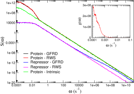
Figure 4: Power spectra of the repressor and protein concentrations obtained for $f=100$, $k_{\text{OC}}=30s^{-1}$, $N_{R}=5$. Data are shown both for the renormalized well-stirred model (RWS) with reaction rates renormalized according to Eqs. 16-17, and for GFRD, taking into account the spatial fluctuations of the repressor molecules explicitly. Also shown is the power spectrum of the intrinsic noise, which is the power spectrum of the protein concentration in the absence of fluctuations in the repressor concentration (extrinsic noise). For large $\omega$, the repressor spectrum (extrinsic noise) differs between the well-stirred and the spatially resolved model. However, this difference does not appear in the power spectra of the protein concentration. The inset shows the frequency-dependent gain $g(\omega)$ (see Eq. 20).

Fig. 4 shows that the power spectrum of the protein concentration in the spatially resolved model is identical to that in the well-stirred model for the entire range of frequencies observed. This confirms the observation in Section VI that the effect of the spatial fluctuations of the repressor molecules on the noise in the protein concentration can by described by a well-stirred model in which the reaction rates for repressor (un)binding to the DNA are properly renormalized.

Fig. 4 also elucidates the reason why a well-stirred model with properly renormalized rate constants for repressor (un)binding can successfully describe the effect of the diffusive motion of the repressor molecules on the noise in gene expression. It is seen that the repressor spectrum for the renormalized well-stirred model is accurately described by a Lorentzian function with a corner frequency $\mu=0.02s^{-1}$, as expected for the dynamics of repressor (un)binding dynamics (see next section). The repressor spectrum of the spatially resolved model fully overlaps with that of the well-stirred model up to a frequency of $\omega\approx 10^{6}{\rm s}^{-1}$, but for higher frequencies it shows a clear deviation from the $\omega^{-2}$ behavior. This deviation is caused by the diffusive motion of the repressor molecules. Indeed, the deviation occurs at frequencies comparable to the inverse of the typical time scale for rapid rebindings ($\sim\mu{\rm s}$). However, this difference between the spectrum of the repressor dynamics in the spatially resolved model and that in the well-stirred model does not manifest itself in the spectra for the protein concentrations of the two respective models, for two reasons: 1) the difference only occurs at high frequencies, i.e. in a frequency regime where the fluctuations only marginally contribute to the noise strength (the difference in area under the curves of the repressor power spectra for the two models is less than $5\%$); 2) the repressor fluctuations in this frequency range are filtered out by the processing network of transcription and translation; as a result of this, the effect of the small difference in area under the curves of the repressor power spectra for the two models is reduced even further. The filtering properties of the processing network are illustrated in the inset of Fig. 4, which shows the transfer function $g(\omega)$ as obtained from $g(\omega)=(S_{P}(\omega)-S_{\text{in}}(\omega))/S_{\text{ex}}(\omega)$ (see Eq. 20). Clearly, the transfer function rapidly decreases as the frequency increases. This shows that the processing network of transcription and translation acts as a low-pass filter, rejecting the high frequency noise in the repressor dynamics that originates from the rapid rebindings.

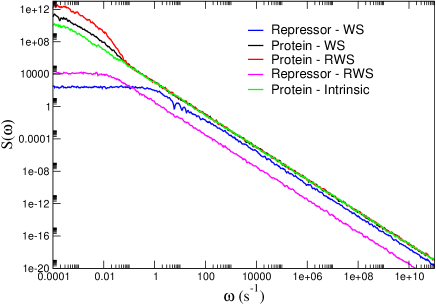
Figure 5: The power spectra for the well-stirred model with unrenormalized rate constants (WS) and for the well-stirred model with renormalized rate constants for repressor (un)binding to (from) the DNA (RWS). The intrinsic noise of gene expression is the same for both models. The extrinsic noise, arising from the repressor dynamics, is, however, markedly different. The repressor spectrum for the well-stirred model with renormalized rate constants has lower corner frequency, but, more importantly, also a higher power at low frequencies. The increased power at low frequencies is not filtered by the processing network and increases the noise in gene expression.

The only effect of the repressor rebindings on the noise in gene expression is thus that it lowers the effective dissociation rate (and association rate), as explained in the previous section. As compared to the well-stirred model with the unrenormalized rate constants for repressor (un)binding, this decreases the corner frequency $\mu$ in the repressor power spectrum (see Fig. 5), but increases the power at low frequencies – recall that for a two-state model, which relaxes mono-exponentially, the power spectrum at zero frequency is $S(\omega=0)=2\sigma^{2}/\mu$, which thus increases as the relaxation rate $\mu=k_{1}+k_{2}$ decreases as a result of the slower binding and unbinding of repressor (see Eq. 24). The higher power in the repressor spectrum at low frequencies for the spatially resolved model and for the well-stirred model with the renormalized rate constants, as compared to that for the well-stirred model with the unrenormalized rate constants, is not filtered by the processing network of transcription and translation and thus manifests itself in the power spectrum of the protein concentration. Spatial fluctuations of gene regulatory proteins thus increase the noise in gene expression by increasing the power of the input signal at low frequencies.

VII.2 Noise propagation

In Fig. 6 we show how fluctuations in the input signal arising from the dynamics of repressor binding and unbinding, are propagated through the different stages of gene expression. In Fig. 6(a) we illustrate how the noise in the repressor concentration (the extrinsic noise) is transferred to the level of transcription. The figure shows for both the spatially resolved model and for the well-stirred model with renormalized rate constants for repressor (un)binding, the power spectrum of the repressor concentration and the spectrum of the concentration of the elongation complex, defined as $[ORp^{*}]+[T]$. It is clear from Fig. 6(a) that already at the level of the elongation complex, the high-frequency noise due to the rapid rebindings is filtered. Transcription can thus already be described by a well-stirred model with properly renormalized rate constants for repressor (un)binding to (from) the DNA.

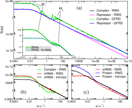
Figure 6: Comparison of the power spectra at different stages of gene expression. (a) Power spectrum for repressor concentration and for the elongation complex $ORp^{*}+T$, both for the well-stirred model with renormalized rate constants (RWS) and for GFRD. Repressor power spectra show a difference between the spatially resolved model and the well-stirred model at high frequencies, due to the diffusion of the repressor molecules. The power spectra for the elongation complexes coincide for the well-stirred and the spatially resolved model. The power spectrum of the elongation complex shows a series of peaks and valleys due to the presence of fixed delays in the dynamics of the elongation complex. (inset) Power spectrum of RNAP dynamics ($OR_{p}+OR_{p}^{*}$). Shown are the power spectra in the presence and absence of fixed delays in the RNAP dynamics. Due to the competition between RNAP and rerepssor for binding to the promoter, the power spectrum is described by a sum of two Lorentzians. (b) Power spectra of the elongation complex and mRNA. Peaks due to the delays in RNAP dynamics are still present in the mRNA dynamics. For high frequencies, the mRNA dynamics is well described by a linear birth-and-death process. (c) Spectra of mRNA and protein. The slow protein dynamics filters out all the peaks resulting from the delays in the RNAP dynamics. The only difference between the full spectrum of the output signal and that of the intrinsic noise is an increased noise at low frequencies, due to the repressor dynamics.

The power spectrum of the elongation complex exhibits two corner frequencies, one around $\omega_{+}\approx 40s^{-1}$ and another one at $\omega_{-}\approx 0.02s^{-1}$. These two corner frequencies arise from the competition between repressor and RNAP for binding to the promoter. To elucidate this, we have plotted in the inset the power spectrum for RNAP bound to the promoter, thus the power spectrum for $[ORp]+[ORp^{*}]$. It is seen that this power spectrum has the same two corner frequencies as that of the elongation complex, showing that their dynamics is dominated by the same processes – repressor binding and RNAP binding to the promoter. These two corner frequencies can be estimated analytically by considering the reactions in Eqs. 3-6 as a three-state system, in which repressor and RNAP compete for binding to the promoter:

$$OR\overset{k_{2}}{\underset{k_{1}}{\rightleftarrows}}O\overset{k_{3}}{\underset{k_{4}}{\rightleftarrows}}ORp^{\prime}.$$ (25)

Here, $ORp^{\prime}=ORp+ORp^{*}$, where $ORp$ denotes the RNAP bound to the promoter in the closed complex and $ORp^{*}$ denotes RNAP bound to the promoter in the open complex. The rate constant $k_{1}$ denotes the rate at which a repressor binds to the promoter; it is given by $k_{1}=k^{\prime}_{fR}[R_{\rm T}]$, where $k^{\prime}_{fR}$ is the renormalized association rate (see Eq. 16). The rate constant $k_{2}$ denotes the renormalized rate for repressor unbinding, $k_{2}=k^{\prime}_{bR}$ (see Eq. 17); $k_{3}=k_{fRp}$ denotes the rate at which RNAP binds to the promoter. The rate constant $k_{4}$ is the rate at which the RNAP leaves the promoter. Since the promoter can become accessible for the binding of another RNAP or repressor by either the dissociation of RNAP from the closed complex or by forming the open complex and then clearing the promoter, this rate is given by $k_{4}=k_{bRp}+(k_{OC}^{-1}+t_{\rm clear})^{-1}$. If promoter clearance would be neglected, then, indeed, $k_{4}=k_{bRp}+k_{OC}$.

The power spectrum of the RNAP dynamics in Eq. 25 can be calculated analytically and is given by a sum of two Lorentzians:

$$S_{ORp^{\prime}}(\omega)=\frac{A\omega_{-}}{\omega_{-}^{2}+\omega^{2}}+\frac{B\omega_{+}}{\omega_{+}^{2}+\omega^{2}},$$ (26)

where $A$ and $B$ are coefficients. The corner frequencies $\omega_{-}$ and $\omega_{+}$ are given by $\omega_{\pm}=(k\pm\sqrt{k^{2}-4h})/2$, where $k=\sum_{i}k_{i}$ and $h=k_{1}k_{4}+k_{2}(k_{3}+k_{4})$. The dynamics of repressor binding and unbinding is much slower than that of RNAP binding and unbinding, meaning that $k_{1},k_{2}\ll k_{3},k_{4}$. This allows us to approximate the corner frequencies as $\omega_{+}=k_{3}+k_{4}$ and $\omega_{-}=k_{2}+k_{1}k_{4}/(k_{3}+k_{4})$. This yields the following expressions for the corner frequencies:

$$\omega_{+} = k_{fRp}+k_{bRp}+(k_{OC}^{-1}+t_{\rm clear})^{-1}$$ (27)

$$\omega_{-} = k_{bR}^{\prime}+k^{\prime}_{fR}[R_{\rm T}][O]^{\prime}.$$ (28)

Here, $[O]^{\prime}\equiv k_{4}/(k_{3}+k_{4})$ is the conditional probability that the promoter is not occupied by the RNAP, given that it is not occupied by repressor; it is given by the occupancy of the promoter by RNAP in the absence of any repressor molecules in the system. We can now see that the highest corner frequency, $\omega_{+}$, describes the fast dynamics of RNAP binding to, and clearing from, the promoter and that the other corner frequency, $\omega_{-}$, represents the slow dynamics of repressor (un)binding to the DNA in the presence of the fast RNAP bindings to the promoter; the lower corner frequency, $\omega_{-}$, is also the corner frequency in the repressor spectrum of the renormalized well-stirred model (see Figs. 4 and 5). In Fig. 6(a) we plot the power spectrum $S_{ORp^{\prime}}(\omega)$ as predicted by the three-state model (Eq. 26; with fitted coefficients $A$ and $B$) on top of the power spectrum obtained from the simulations and find excellent agreement. We also show the power spectra when we neglect the delay due to promoter clearance. As expected, in the absence of the delay due to promoter clearance, the lower corner frequency, $\omega_{-}$, and, to a smaller extent, the higher corner frequency, $\omega_{+}$, are shifted to higher frequencies.

The power spectrum of the elongation complex in Fig. 6(a) contains information that is not easily observed in the time domain and could as a result be helpful in the interpretation of the results. It is seen that there are two series of peaks. Those are associated with the two processes with fixed time delays. The first process is the promoter clearance, which takes a fixed time $t_{\rm clear}$. Indeed, the first peak in the corresponding series of peaks in the power spectrum of the elongation complex, is at $\omega\approx 2\pi/(t_{\text{clear}})=6.3s^{-1}$; the other peaks in the series are the higher harmonics that naturally arise for processes with fixed time delays. The second process is the transcript elongation process. After the elongation complex has been formed, it takes a fixed time $t_{\rm clear}+t_{\rm elon}$ before the full transcript is formed and the RNAP dissociates from the DNA; the first valley of the corresponding series of peaks/valleys is, indeed, at $\omega\approx 2\pi/(t_{\rm clear}+t_{\rm elon})=0.2{\rm s}^{-1}$. While the frequency $2\pi/t_{\rm clear}$ yields, to a good approximation, the rate at which the elongation complex signal increases, the frequency $2\pi/(t_{\rm clear}+t_{\rm elon})$ corresponds to the frequency at which the elongation complex signal decreases; this explains why the shapes of the respective series of peaks and valleys are reciprocal. Lastly, the reason that both peaks and valleys are broadened is that the delay in the formation of the elongation complex is not fully deterministic: the duration of the delay is not only determined by the promoter clearance time, which, indeed, is fixed, but also by the time it takes for another RNAP to bind the DNA and then form the open complex – in the absence of repressor, the average frequency at which an elongation complex is formed is given by $2\pi/(k_{\rm fRp}^{-1}+k_{\rm OC}^{-1}+t_{\rm clear})$ (see also Eqs. 4– 6). Both RNAP binding and open complex formation are modeled as Poisson processes, and this leads to a distribution of delay times for the formation of the elongation complex.

In Fig. 6(b) and (c), we examine how the noise in the dynamics of the elongation complex propagates to the level of mRNA and protein dynamics. In Fig. 6(b), we compare the full power spectrum of the mRNA concentration with that of the elongation complex – the input signal (extrinsic noise) for the mRNA signal – and that of the intrinsic noise of the mRNA signal; to compute the intrinsic noise, we have modeled the mRNA dynamics as a birth-and-death process (see Eq. 22) with a production rate as given by the average production rate for the full system in Eqs. 3-11. As expected, for higher frequencies ($\omega>0.1{\rm s}^{-1}$), the full spectrum of mRNA overlaps almost fully with that of the intrinsic noise, although some traces of the input signal (the elongation complex) are still apparent in this high frequency regime; these are the peaks at $\omega\approx 6.3{\rm s}^{-1}$ corresponding to promoter clearance. At lower frequencies ($\omega<0.1{\rm s}^{-1}$), the noise in the mRNA signal is dominated by the extrinsic noise, which is the noise in the elongation complex (the input signal). Indeed, both the spectrum of the elongation complex and that of mRNA have a corner frequency at $\omega_{-}$, which, as discussed above, arises from the slow repressor (un)binding to the DNA in the presence of the fast DNA-(un)binding kinetics of RNAP.

Fig. 6(c) shows how the noise in the mRNA concentration is propagated to that in the protein concentration. Again, at higher frequencies, the spectrum of the protein concentration coincides with that of the intrinsic noise of protein synthesis, which, as above for mRNA, has been computed by modeling protein production as a birth-and-death process; note also that the remnants of operator clearance (the peaks in the spectrum at $\omega\approx 6.3{\rm s}^{-1}$) have been filtered by the slow protein dynamics. Only for frequencies smaller than $\omega\approx 0.1{\rm s}^{-1}$, does the extrinsic noise – the noise in the mRNA concentration – strongly contribute to the noise in the protein concentration. A careful inspection of the protein spectrum shows that it has a “corner” at $\omega_{-}$, which arises from the repressor DNA-(un)binding dynamics (the extrinsic noise), and one, albeit much less visible, at $\omega\approx k_{\rm dp}=2\times 10^{-4}{\rm s}^{-1}$, which is due to the intrinsic dynamics of protein degradation.

VIII Discussion and Outlook

Our analysis reveals that at high frequencies both mRNA and protein synthesis are well described by a linear birth-and-death model. In this frequency regime, the effect of spatial fluctuations, originating from the rapid repressor rebindings, is completely filtered by the slow dynamics of transcription and translation. These rebindings do, however, decrease the effective rate at which the repressor molecules associate with, and dissociate from, the promoter. This increases the intensity of the extrinsic (repressor) noise in the low frequency regime. Moreover, the low-frequency fluctuations in the repressor binding do propagate through the different stages of gene expression. In particular, they lead to sharp bursts in the production of mRNA and protein. These bursts increase the noise intensity at the lower frequencies in the noise spectrum of mRNA and protein. And since the noise strength $\sigma^{2}$ is dominated by fluctuations in the low-frequency regime, spatial fluctuations ultimately strongly increase the noise in mRNA and protein concentration.

Recently, experiments have been performed, in which the synthesis of individual mRNA transcripts Golding et al. (2005) and individual protein molecules Yu et al. (2006) could be detected. The systems in these studies were very similar to that studied here: a gene under the control of a (Lac) repressor. These studies unambiguously demonstrated that transcription Golding et al. (2005) and translation can occur in bursts Yu et al. (2006). Our simulation results show that spatial fluctuations of the repressor molecules might be responsible for this. Indeed, our results strongly suggest that spatial fluctuations are the dominant source of noise in gene expression in these systems.

The spatial fluctuations due to diffusion of the repressor molecules could have significant implications for the functioning of gene regulatory networks. Under some conditions, it might be crucial that the protein number is not only low on average, but remains low at all times. For instance, if the protein itself functions as a transcription factor, it might by accident induce the expression of another gene, when, due to a fluctuation, its concentration crosses a particular activation threshold. Thus, not all combinations of repressor copy number $N_{R}$ and repressor backward rate $k_{\text{bR}}$ that obey Eq. 14 and thus have the same average repression strength, are necessarily equivalent in terms of function when diffusion is taken into account. If the fluctuations in the repressed state need to be small, then the cell could increase the number of repressors and decrease the binding affinity to the operator site, such that the repressor molecules stay bound to the DNA only briefly. Alternatively, the cell could minimize the effect of fluctuations by reducing the rate at which the open complex is formed by RNAP – our analysis shows that the process of open complex formation can act as a strong low-pass filter.

The rapid rebindings observed in our simulations are a general phenomenon. We now address the question when the effect of spatial fluctuations due to diffusion can be described by a well-stirred model in which the association and dissociation rates are renormalized. In the current problem, the rebinding time for a dissociated repressor is exceedingly short. As a consequence, the probability that a RNAP binds to the promoter during this time, is vanishingly small. This is precisely the reason that the effective dissociation rate is simply the bare dissociation rate divided by the number of rebindings (see Eq. 18); the effective association rate is renormalized accordingly, because the equilibrium constant should remain unchanged (see Eq. 19). The success of the renormalized well-stirred model is thus a result of the strong separation of time scales – the time scale of repressor rebinding is well separated from that of RNAP binding.

The separation of time scales also makes it possible to account for the effect of spatial fluctuations by renormalizing the association and dissociation rates in other cases. For instance, we have simulated a system in which repression occurs in a cooperative manner. In this system, the repressor backward rate is smaller when two repressors are bound to the operator than when a single repressor is bound. However, when one of the two repressors dissociates, its rebinding time is so short that the probability for the other repressor to dissociate in the mean time, is negligible for reasonable values of cooperativity. As a result, the effect of spatial fluctuations can be described by a well-stirred model with properly renormalized reaction rates. We have also studied a system in which the expression of a gene is not under the control of a repressor, but rather under the control of an activator. Also in this system, diffusion of the transcription factors leads to an enhancement of noise in gene expression through a similar mechanism.

Do these observations imply that the effect of spatial fluctuations can always be described by a well-stirred model? In the system studied here, the ligand (repressor) molecules bind to a single site. We expect that the effect of spatial fluctuations becomes more intricate when the number of binding sites for a particular ligand increases – the binding of the ligand to the different sites will then exhibit correlations. This could be important when the ligand binds to receptors that occur in dense clusters, as in bacterial chemotaxis D. Bray, M. D. Levin, and C. J. Morton-Firth (1998); Andrews (2005) and in the immune response Valitutti et al. (1995). In gene regulatory networks this effect could also be significant. Recently, we have shown that in E. coli, pairs of co-regulated genes – genes that are controlled by a common transcription factor – tend to lie exceedingly close to each other on the genome Warren and ten Wolde (2004): their promoter regions are often separated by a distance smaller than a few hundred base pairs. It is conceivable that spatial fluctuations of the transcription factors introduce correlations between the noise in the expression of these pairs of co-regulated genes. This study also revealed that pairs of genes that regulate each other, often lie close together, again suggesting that the diffusive motion of transcription factors could be important for the functioning of gene regulatory networks Warren and ten Wolde (2004).

Even in the case of a single gene, the effect of spatial fluctuations is expected to be more subtle than that reported here. In this study, the operator is modeled as a spherical site. However, as mentioned in section II.1, transcription factors are believed to find their operator site via a combination of free 3D diffusion and 1D sliding along the DNA. While on length scales larger than the sliding distance this process is indeed essentially 3D diffusion, on length and time scales smaller than the sliding distance and sliding time, respectively, the dynamics is more complicated. We expect that sliding could have two important effects. First, it will increase the number of rebindings – the probability that in 1D a random walker returns to the origin is one, while in 3D there is a finite probability that it will escape and never return. Secondly, sliding is expected to also increase the duration of the rebindings, especially when diffusion along the DNA is much slower than diffusion in the cytoplasm. It is thus conceivable that with sliding, the non-exponential relaxation of the operator state, arising from the rebindings, shifts to lower frequencies (see Fig. 4), where fluctuations in the operator state are not filtered out. In addition, it is possible that with sliding, RNAP and repressor compete for binding to the promoter on similar time scales, which would mean that the effective dissociation rate is no longer simply given by the bare dissociation rate divided by the number of rebindings. Indeed, under these conditions, the effect of spatial fluctuations is likely to become non-trivial, and describing it would probably require a spatially resolved model. We leave this for future work.

Finally, we address the question whether spatial fluctuations, and, more in particular, the rebindings, could be studied experimentally. Interestingly, recent biochemical data on the restriction enzyme EcoRV suggests that after an initial dissociation, 10-100 rebindings occur before the enzyme escapes into the bulk solution Stanford et al. (2000); Gowers et al. (2005), in good agreement with the average number of rebindings calculated in section VI. However, in our gene expression model, the rebinding times are so short that it would seem difficult to probe the repressor rebindings directly in an experiment. In fact, reaction rates measured biochemically will probably already be corrected for according to Eqs. 16 and 17. Sliding along the DNA, however, may extend the rebinding times to accessible experimental time scales. Moreover, recent experiments suggest that the motion of proteins in the nucleoid might be sub-diffusive, which would increase the importance of the rebindings Golding and Cox (2006). Recently, magnetic tweezer experiments on a mechanically stretched, supercoiled, single DNA have made it possible to study the kinetics of the open complex formation and promoter clearance Revyakin et al. (2004). Performing these experiments on a promoter that is under the control of a repressor, seems a promising approach for studying the effect of spatial fluctuations due to the diffusive motion of transcription factors on the dynamics of gene expression.

Appendix Computing Power Spectra

The power spectrum of the time trace of the copy number $X(t)$ of a species $\rm X$ can be efficiently computed by exploiting the fact that in between the times $t_{k}$ the signal $X(t)$ is constant. The Fourier Transform $S_{\rm X}(\omega)$ of $X(t)$ is

$$\tilde{X}(\omega)=\int X(t)e^{-i\omega t}dt=\sum_{k}\int_{t_{k-1}}^{t_{k}}X_{k}e^{-i\omega t}dt.$$ (29)

As $X(t)$ is constant within every interval $\{t_{k-1},t_{k}\}$, the integration can easily be performed:

$$\tilde{X}(\omega)=\sum_{k}X_{k}\frac{1}{-i\omega}(e^{-i\omega t_{k}}-e^{-i\omega t_{k-1}}).$$ (30)

Shifting up by one the index $j$ in the second part of the sum, we obtain:

$$\tilde{X}(\omega)=\frac{1}{i\omega}\sum_{k}(X_{k+1}-X_{k})(e^{-i\omega t_{k}}).$$ (31)

The real and imaginary parts of the Fourier Transform are thus:

$$\Re{[\tilde{X}(\omega)]} = \frac{1}{\omega}\sum_{k}\delta_{k}(\sin{\omega t_{k}})$$ (32)

$$\Im{[\tilde{X}(\omega)]} = \frac{1}{\omega}\sum_{k}\delta_{k}(\cos{\omega t_{k}}),$$ (33)

where we have defined $\delta_{k}=X_{k+1}-X_{k}$. The Power spectrum $S_{\rm X}(\omega)=\Re{[\tilde{X}(\omega)]}^{2}+\Im{[\tilde{X}(\omega)]}^{2}$ is thus given by

$$S_{\rm X}(\omega)=\left(\frac{1}{\omega}\sum_{k}\delta_{k}\cos(\omega t_{k})\right)^{2}+\left(\frac{1}{\omega}\sum_{k}\delta_{k}\sin(\omega t_{k})\right)^{2}.$$ (34)

The Fourier Transforms were computed at 10000 logarithmically spaced angular frequencies starting from $\omega_{\text{min}}=10\cdot 2\pi/T$, where $T$ is the total length of the signal. Power spectra obtained according to Eq. 34 were filtered with a box average over 20 neighboring points.

References

- McAdams and Arkin (1997) H. H. McAdams and A. Arkin, Proc. Natl. Acad. Sci. USA 94, 814 (1997).
- Elowitz et al. (2002) M. B. Elowitz, A. J. Levine, E. D. Siggia, and P. S. Swain, Science 297, 1183 (2002).
- Ozbudak et al. (2002) E. M. Ozbudak, M. Thattai, I. Kurtser, A. D. Grossman, and A. van Oudenaarden, Nat. Gen. 31, 69 (2002).
- Rao et al. (2002) C. V. Rao, D. M. Wolf, and A. P. Arkin, Nature 420, 231 (2002).
- Kaern et al. (2005) M. Kaern, T. C. Elston, W. J. Blake, and J. J. Collins, Nat. Rev. Gen. 6, 451 (2005).
- van Kampen (2001) N. G. van Kampen, Stochastic Processes in Physics and Chemistry (Elsevier, Amsterdam, 2001).
- Gillespie (1976) D. T. Gillespie, J. Comp. Phys. 22, 403 (1976).
- Swain et al. (2002) P. S. Swain, M. B. Elowitz, and E. D. Siggia, Proc. Natl. Acad. Sci. USA 99, 12795 (2002).
- Paulsson (2004) J. Paulsson, Nature 427, 415 (2004).
- Rosenfeld et al. (2005) N. Rosenfeld, J. W. Young, U. Alon, P. S. Swain, and M. Elowitz, Science 307, 1962 (2005).
- Elf and Ehrenberg (2004) J. Elf and M. Ehrenberg, Sys. Biol. 2, 230 (2004).
- Ander et al. (2004) M. Ander, P. Beltrao, B. D. Ventura, J. Ferkinghoff-Borg, M. Foglierini, A. Kaplan, C. Lemerle, I. Tomas-Oliveira, and L. Serrano, Sys. Biol. 1, 129 (2004).
- Andrews and Bray (2004) S. S. Andrews and D. Bray, Physical Biology 1, 137 (2004).
- van Zon and ten Wolde (2005a) J. S. van Zon and P. R. ten Wolde, Phys. Rev. Lett. 94, 018104 (2005a).
- van Zon and ten Wolde (2005b) J. S. van Zon and P. R. ten Wolde, J. Chem. Phys. 123, 234910 (2005b).
- M. S. H. Ko (1991) M. S. H. Ko, J. Theor. Biol. 153, 181 (1991).
- Kepler and Elston (2001) T. B. Kepler and T. C. Elston, Biophys. J. 81, 3116 (2001).
- Karmakar and Bose (2004) R. Karmakar and I. Bose, Physical Biology 1, 197 (2004).
- Pirone and Elston (2004) J. R. Pirone and T. C. Elston, J. Theor. Biol. 226, 111 (2004).
- Simpson et al. (2004) M. L. Simpson, C. D. Cox, and G. S. Sayler, J. Theor. Biol. 229, 383 (2004).
- Bialek and Setayeshgar (2005) W. Bialek and S. Setayeshgar, Proc. Natl. Acad. Sci. USA 102, 10040 (2005).
- Hornos et al. (2005) J. E. M. Hornos, D. Schultz, G. C. P. Innocentini, A. M. W. J. Wang, J. N. Onuchic, and P. G. Wolynes, Phys. Rev. E 72, 051907 (2005).
- Metzler (2001) R. Metzler, Phys. Rev. Lett. 87, 068103 (2001).
- Record et al. (1996) M. Record, W. S. Reznikoff, M. L. Craig, K. L. McQuade, and P. J. Schlax, in Escherichia coli and Salmonella, edited by F. C. Neidhardt et al. (ASM Press, Washington D.C., 1996), pp. 792 – 821, 2nd ed.
- Austin et al. (2006) D. W. Austin, M. S. Allen, J. M. Coolum, R. D. Dar, J. R. Wilgus, S. G. Sayler, N. F. Sarmatova, C. D. Cox, and M. L. Simpson, Nature 439, 608 (2006).
- Revyakin et al. (2004) A. Revyakin, R. H. Ebright, and T. R. Strick, Proc. Natl. Acad. Sci. USA 101, 4776 (2004).
- Riggs et al. (1970) A. D. Riggs, S. Bourgeois, and M. Cohn, J. Mol. Biol. 53, 401 (1970).
- Berg et al. (1981) O. G. Berg, R. B. Winter, and P. H. von Hippel, Biochemistry 20, 6929 (1981).
- Halford and Marko (2004) S. E. Halford and J. F. Marko, Nucl. Acids Res. 32, 3040 (2004).
- Gerland et al. (2002) U. Gerland, J. Moroz, and T. Hwa, Proc. Natl. Acad. Sci. USA 99, 12015 (2002).
- Coppey et al. (2004) M. Coppey, O. Bénichou, R. Voituriez, and M. Moreau, Biophys. J. 87, 1640 (2004).
- Slutsky and Mirny (2004) M. Slutsky and L. A. Mirny, Biophys. J. 87, 4021 (2004).
- Klenin et al. (2006) K. V. Klenin, H. Merlitz, J. Langowski, and C.-X. Wu, Phys. Rev. Lett. 96, 018104 (2006).
- Hu et al. (2006) T. Hu, A. Grosberg, and B. I. Shklovskii, Biophys. J. 90, 2731 (2006).
- Stanford et al. (2000) N. P. Stanford, M. D. Szczelkun, J. F. Marko, and S. E. Halford, EMBO J. 19, 6546 (2000).
- Gowers et al. (2005) D. M. Gowers, G. G. Wilson, and S. E. Halford, Proc. Natl. Acad. Sci. USA 102, 15883 (2005).
- Elowitz et al. (1999) M. B. Elowitz, M. G. Surette, P.-E. Wolf, J. B. Stock, and S. Leibler, J. Bacteriol. 181, 197 (1999).
- Bremer et al. (2003) H. Bremer, P. Dennis, and M. Ehrenberg, Biochimie 84, 597 (2003).
- McClure (1983) M. R. McClure, in Biochemistry of Metabolic Processes, edited by D. L. F. Lennon, F. W. Stratman, and R. N. Zahlten (Elsevier, New York, 1983), pp. 207 – 217.
- Kushner (1996) S. Kushner, in Escherichia coli and Salmonella, edited by F. C. Neidhardt et al. (ASM Press, Washington D.C., 1996), pp. 849 – 860, 2nd ed.
- Vilar and Leibler (2003) J. Vilar and S. Leibler, J. Mol. Biol. 331, 981 (2003).
- Gillespie (1977) D. T. Gillespie, J. Phys. Chem. 81, 2340 (1977).
- M. Eigen (1974) M. Eigen, Diffusion control in biochemical reactions (Plenum Press, New York, 1974).
- D. Shoup and A. Szabo (1982) D. Shoup and A. Szabo, Biophys. J. 40, 33 (1982).
- M. Smoluchowski (1917) M. Smoluchowski, Z. Phys. Chem. 92, 129 (1917).
- Kim and Shin (1999) H. Kim and K. J. Shin, Phys. Rev. Lett. 82, 1578 (1999).
- Pedraza and van Oudenaarden (2005) J. M. Pedraza and A. van Oudenaarden, Science 307, 1965 (2005).
- Detwiler et al. (2000) P. B. Detwiler, S. Ramanathan, A. Sengupta, and B. I. Shraimann, Biophys. J. 79, 2801 (2000).
- Shibata and Fujimoto (2005) T. Shibata and K. Fujimoto, Proc. Natl. Acad. Sci. USA 102, 331 (2005).
- Tănase-Nicola et al. (2005) S. Tănase-Nicola, P. B. Warren, and P. R. ten Wolde, q-bio.BM/0508027 (2005).
- Warren et al. (2005) P. B. Warren, S. Tănase-Nicola, and P. R. ten Wolde, q-bio.SC/0512041 (2005).
- Golding et al. (2005) I. Golding, J. Paulsson, S. M. Zawilski, and E. C. Cox, Cell 123, 1025 (2005).
- Yu et al. (2006) J. Yu, J. Xiaojia, K. Lao, and X. Xie, Science 311, 1600 (2006).
- D. Bray, M. D. Levin, and C. J. Morton-Firth (1998) D. Bray, M. D. Levin, and C. J. Morton-Firth, Nature 393, 85 (1998).
- Andrews (2005) S. S. Andrews, Physical Biology 2, 111 (2005).
- Valitutti et al. (1995) S. Valitutti, S. Müller, M. Cella, E. Padovan, and A. Lanzavecchia, Nature 375, 148 (1995).
- Warren and ten Wolde (2004) P. B. Warren and P. R. ten Wolde, J. Mol. Biol. 342, 1379 (2004).
- Golding and Cox (2006) I. Golding and E. C. Cox, Phys. Rev. Lett. 96, 098102 (2006).