Abstract

The spectrotemporal receptive field (STRF) provides a versatile and integrated, spectral and temporal, functional characterization of single cells in primary auditory cortex (AI). In this paper, we explore the origin of, and relationship between, different ways of measuring and analyzing an STRF. We demonstrate that STRFs measured using a spectrotemporally diverse array of broadband stimuli — such as dynamic ripples, spectrotemporally white noise, and temporally orthogonal ripple combinations (TORCs) — are very similar, confirming earlier findings that the STRF is a robust linear descriptor of the cell. We also present a new deterministic analysis framework that employs the Fourier series to describe the spectrotemporal modulations contained in the stimuli and responses. Additional insights into the STRF measurements, including the nature and interpretation of measurement errors, is presented using the Fourier transform, coupled to singular-value decomposition (SVD), and variability analyses including bootstrap. The results promote the utility of the STRF as a core functional descriptor of neurons in AI.

Key Words: spectrotemporal receptive field, modulation transfer function, auditory cortex, ripple, variability, singular-value decomposition, ferret

1 Introduction

It has been over twenty years since the spectrotemporal receptive field (STRF) was conceived to describe and measure auditory neurons’ joint sensitivity to the spectral and temporal dimensions of acoustical energy (Hermes et al.,, 1981; Aertsen and Johannesma, 1981b, ; Smolders et al.,, 1979; Eggermont et al.,, 1981; Johannesma and Eggermont,, 1983). It was specifically associated with (1) stimuli characterized by randomly varying spectrotemporal features, and (2) an approach labeled reverse correlation, by which the neuron informs the experimenter, via action potentials, of the features that were of interest to it (de Boer and de Jongh,, 1978; Eggermont et al., 1983b, ). The STRF offered a view of neuronal function that complemented, and was usually consistent with, that obtained using classical stimuli such as tones (tuning curves and rate-level functions), clicks (impulse responses), and noise (bandwidth sensitivity). In addition, it neatly fit within an analytical framework, bolstered by the fields of time-frequency analysis (Cohen,, 1995) and nonlinear systems theory (Eggermont,, 1993), within which the functionality of neurons could, in principle, be systematically explored to any level of detail.

The term “STRF” does not denote here the full complex (likely nonlinear) receptive field of an auditory neuron. Rather it is a technical term that has traditionally been used to refer specifically to the linear relationship between the time-dependent spike rate of a neuron and the time- and frequency-dependent energy — in short, the dynamic spectrum — of a stimulus. In order to measure the STRF, the reverse-correlation approach prescribes computing the average dynamic spectrum of those portions of a stimulus preceding the neuron’s spikes. In this context, the STRF is commonly interpreted as the spectrotemporal pattern that optimally activates a neuron (Young,, 1998). Theoretically, as long as all patterns occur randomly, independently, and equiprobably, the STRF can be revealed by this “spike-triggered average” (Eggermont,, 1993).

As with tuning curves, rate-level functions, and other commonly used neuronal response measures, the STRF provides only a limited view of the receptive field of a neuron, one that is useful only within the context of the experiment or the nature of information sought from it. For example, tuning curves are useful as approximate indicators of a unit s BF and bandwidth, but are largely irrelevant as a gauge of its dynamic range and temporal properties. Similarly, the STRF is a useful measure of spectrotemporal features likely to drive a cell s responses. However, being a measure of the linear component of the stimulus-response relationship, it is mostly effective in predicting the linear aspects of the responses, predictions that can be accurate if the non-linear portions are small or are well known and can be accounted for in the measurement (e.g., spike-rate rectification and saturation). In some cases, the linear component of the response is small and hence one does not expect clean and reliable STRF measurements, i.e., the STRFs exhibit significant randomness or high variability across presentations, or are poor predictors of responses to novel stimuli. Examining these sources of variability and prediction errors provides useful information regarding the limitations of the STRF and ways to extend it beyond the linear domain.

Although the STRF has been slow to mature, it is now increasingly used to study the physiology of central auditory neurons. In retrospect, the often slow pace of progress can be partially attributed to the reverse-correlation methodology, which remains fairly opaque. In particular, reverse correlation provides no straightforward formal basis for describing the effectiveness of, or relations between, specific stimuli, because only the average statistics of stimuli are specified. For example, Gaussian broad-band noise, the “ideal” stimulus for reverse-correlation, is often ineffective when applied to central auditory neurons (but see (Keller and Takahashi,, 2000)). Meanwhile, a range of other stimuli and associated techniques have been auditioned, modulated broad-band noise (Miller et al.,, 2002; Escabí and Schreiner,, 2002), random sequences of tones or chords (Aertsen and Johannesma, 1981a, ; Epping and Eggermont,, 1985; Schafer et al.,, 1992; deCharms et al.,, 1998; Theunissen et al.,, 2000; Rutkowski et al.,, 2002), and natural stimuli (Aertsen and Johannesma, 1981a, ; Yeshurun et al.,, 1987; Schafer et al.,, 1992; Theunissen et al.,, 2000; Sen et al.,, 2001). While it is sometimes implied that the auditory system processes different stimuli differently, it has not been made clear, because of the lack of vocabulary, to what extent different stimulation methods should yield different results. Additionally, most of the employed stimuli share randomness in their spectrotemporal design, in accordance with the reverse-correlation approach, but this style of stimulation is bound to be inefficient (Victor and Knight,, 1979; Sutter,, 1992).

Because of these shortcomings, we endeavored to record a deterministic and analytical reformulation of spectrotemporal reverse correlation (Klein et al.,, 2000). The roots of this new methodology are in the Fourier-based analysis (Papoulis,, 1962) of any given stimulus in terms of its spectrotemporal modulation frequency content. Each spectrotemporal modulation frequency is the conjunction of a spectral and a temporal modulation frequency; the higher the spectral modulation frequency, the sharper the spectral feature (e.g., sharp peaks or edges in the spectrum), and the higher the temporal modulation frequency, the more abruptly that feature changes in time. As a population, the strongest phase-locked response in central auditory neurons occurs over a select range of low spectral and temporal modulation frequencies (Rees and Moller,, 1983; Shamma et al.,, 1995; Schreiner and Calhoun,, 1995; Kowalski et al., 1996a, ; Depireux et al.,, 2001; Sen et al.,, 2001; Miller et al.,, 2002; Escabí and Schreiner,, 2002). Not surprisingly, the most fruitful stimuli have had spectrotemporal modulation frequencies concentrated within this range. Our approach extends these past successes by making explicit the relations between the spectrotemporal modulation frequency content of a stimulus, the stimulus duration and bandwidth, and the accuracy of the STRF measurement. This enables the flexible design of diverse stimuli that minimize both stimulation time and measurement error, within the constraints of a particular experiment. These constraints include information about not only the STRF, but also about the nonlinear and stochastic aspects of the stimulus-response transformation, which are not directly described by the STRF. Another important advantage of this methodology is that it can be used to describe the mechanics of STRF measurement with any given stimulus, thus providing a language with which apparently disparate methods can be discussed.

We focus in this article on three specific types of stimuli with increasing level of complexity, applied in primary auditory cortex (AI) of the anesthetized ferret. At one extreme are the dynamic ripple stimuli (Kowalski et al., 1996a, ; Kowalski et al., 1996b, ; Depireux et al.,, 2001), which each consist of a single spectrotemporal modulation frequency. At the other extreme is spectrotemporally white noise (STWN), which contains many superimposed spectrotemporal modulation frequencies. Intermediate are temporally orthogonal ripple combinations (TORCs), consisting of special combinations of several spectrotemporal modulation frequencies each. We shall explore the relations between these stimuli, and compare the responses they evoke and the resulting STRF measurements. Among the issues addressed are the similarity between the STRF measurements, their fidelity and noise-robustness, their susceptibility to common neuronal nonlinearities, and the expected amount of data necessary to achieve an measurement with a desired level of accuracy. The methods used to address these issues are quite general, though the specific findings apply only to the population of neurons in AI studied here.

2 Methods

2.1 Theory

In this section, we outline the methodological basis of this study. Its key element is an analytical description of the stimulus-to-response transformation, in terms of the processing of spectrotemporal modulation frequencies. In this context, the result of reverse correlation is derived, first assuming that the response is deterministically and linearly related to the stimulus, and then considering the separate effects of response variability and nonlinearity.

At the core of the STRF-based model of neural functionality is the following equation:

$$r(t)=\int{\int{h(\tau,x)\cdot s(t-\tau,x)\,d\tau}\,dx},$$ (1)

where the neuronal response $r$ at any time $t$ is the linear integration of influences arising from stimulus energy $s$ at different tonotopic locations $x$ (here corresponding to the logarithm of frequency) and different times in the past $\tau$. The strength and nature of the influences — whether they are excitatory (positive), or suppressive or inhibitory (negative) — is described by the STRF as denoted by $h(\tau,x)$. In the context of reverse correlation, $r(t)$ is typically taken to be the time-dependent spike rate of a neuron (Eggermont et al., 1983a, ; Keller and Takahashi,, 2000; Sen et al.,, 2001).

2.1.1 The Linear Processing of Spectrotemporal Modulation Frequencies

Our analytical description of dynamic spectra is based upon the Fourier series (Papoulis,, 1962), using elemental Fourier components which are cosine waves as a function of both $t$ and $x$: $a\cdot cos(2\pi wt+2\pi\Omega x+\psi)$. The wave has a peak value of $a$ and starting phase $\psi$. The wave frequency is $w$ cycles/second (Hz) along $t$ and $\Omega$ cycles/octave (cyc/oct) along $x$. Since the dynamic spectrum details the modulation of acoustic energy as a function of both $x$ and $t$, these frequencies are referred to as modulation frequencies: spectral ($\Omega$) and temporal ($w$). A single Fourier component is said to consist of a single spectrotemporal modulation frequency, defined by a specific $(w,\Omega)$ pair. Just as a sum of pure tones of various frequencies, amplitudes, and phases can describe any acoustic waveform over a finite duration, a sum of various spectrotemporal modulation frequencies (with appropriate amplitudes and phases) can describe any dynamic spectrum over a finite duration $T$ and bandwidth $X$. Further, just as the frequency content of an acoustic waveform (i.e., the amplitudes and phases of its constituent tones) is described by its (Fourier) spectrum, the spectrotemporal modulation frequency content of a dynamic spectrum is described by its spectrotemporal modulation spectrum $S$.

When the STRF is recast as operating upon $S$, one arrives at a complementary description called the spectrotemporal modulation transfer function $H$. $H[w,\Omega]$, which is the 2-D Fourier transform of the STRF $h(t,x)$, details the linear component of neural processing of spectrotemporal modulation frequencies. Such processing is already under study in auditory neurophysiology (Kowalski et al., 1996a, ; Kowalski et al., 1996b, ; Depireux et al.,, 2001; Miller et al.,, 2001, 2002; Escabí and Schreiner,, 2002) and psychoacoustics (Chi et al.,, 1999), and is also being investigated for various signal-processing tasks, including audio coding (Atlas and Shamma,, 2003; Klein et al.,, 2003) and speech recognition (Hermmansky,, 1999; Nadeu et al.,, 2001; Kleinschmidt and Gelbart,, 2002; Kleinschmidt,, 2002).

$S$ and $H$ are mathematically defined as follows. Consider a dynamic spectrum $s(t,x)$ and an STRF $h(t,x)$, both given over a finite range of $T$ seconds and $X$ octaves. Using the exponential form of the Fourier series, $s$ can be expressed by the sum

$$s(t,x)=\sum\limits_{k=-\infty}^{\infty}\sum\limits_{l=-\infty}^{\infty}\left(a[w_{k},\Omega_{l}]e^{j\psi[w_{k},\Omega_{l}]}\right)e^{j2\pi(w_{k}t+\Omega_{l}x)},$$ (2)

where $e$ is the base of the natural logarithm, $j=\sqrt{-1}$, $k$ and $l$ are integers, $w_{k}=k/T$, and $\Omega_{l}=l/X$. This is perhaps the simplest form of the Fourier series to use; ironically it employs “complex” exponential functions. These functions are related to the real-valued Fourier components through the trigonometric identity $cos(\phi)=\frac{1}{2}\left(e^{j\phi}+e^{-j\phi}\right)$, etc. Accordingly, each term in this sum, indexed by $k$ and $l$, has a complex-conjugate counterpart, indexed by $-k$ and $-l$, such that $a[w_{k},\Omega_{l}]=a[w_{-k},\Omega_{-l}]$ and $\psi[w_{k},\Omega_{l}]=-\psi[w_{-k},\Omega_{-l}]$. Henceforth we will simplify the notation by dropping the $k$ and $l$ subscripts, however keeping in mind that $w$ and $\Omega$ are discrete-valued variables (as indicated by the square brackets). Thus, the amplitudes and phases of the modulation-frequency components are given by $a[w,\Omega]$ and $\psi[w,\Omega]$, which together form $S[w,\Omega]=a[w,\Omega]e^{j\psi[w,\Omega]}$. As for the STRF, its Fourier series description can be represented by the same sinusoidal components, but with different amplitudes $b[w,\Omega]$ and phases $\theta[w,\Omega]$, which together form $H[w,\Omega]=b[w,\Omega]e^{j\theta[w,\Omega]}$. As we’ll see, $b$ generally describes describes the strength of the response to particular spectrotemporal modulation frequencies, while $\theta$ describes the timing of the response.

In practice, $s(t,x)$ is represented on a computer by discrete samples, $s[t_{k},x_{l}]=s(k\Delta_{t},l\Delta_{x})$, taken at a rate of $1/\Delta_{t}$ samples/second and $1/\Delta_{x}$ samples/octave, where $k$ and $l$ are integers. Again, we will drop the $k$ and $l$ subscripts, however keeping in mind that $t$ and $x$ are now discrete-valued variables. By the sampling theorem (Oppenheim and Schafer,, 1989), this assumes that $S$ is sufficiently smooth; that is, it can be described by a limited number of temporal and spectral modulation frequencies no higher than $1/(2\Delta_{t})$ and $1/(2\Delta_{x})$, respectively. Within these limits, $S[w,\Omega]$ is then obtained by computing the Discrete Fourier Transform (DFT) of $s[t,x]$ (using the Fast Fourier Transform, or FFT, algorithm) (Oppenheim and Schafer,, 1989). Analogously, $H[w,\Omega]$ is obtainable via the (Discrete) Fourier Transform of the STRF $h[t,x]$.

Since the response, $r(t)$, depends only on time, its Fourier-series description utilizes only temporal modulation frequencies. It can be derived by inserting the Fourier-series descriptions of $s$ and $h$ into Eq. (1) and carrying out the integration. The result is that the Fourier Transform of the sampled response $r[t]$ has the form

$$R[w]=\sum\limits_{\Omega}{H[w,-\Omega]\cdot S[w,\Omega]}=\sum\limits_{\Omega}{H[w,\Omega]\cdot S[w,-\Omega]}$$ (3)

Recall that in Eq. (1) the response was obtained by integrating over the spectral axis ($x$) after temporally convolving the dynamic spectrum with the STRF; here, the convolution is realized via the multiplication of Fourier Transforms (Oppenheim and Schafer,, 1989), and the integration over $x$ is replaced by a summation over $\Omega$ . Therefore, each frequency $w$ in the response results from all spectrotemporal modulation frequencies in the stimulus sharing the same temporal component $w$.

2.1.2 Fourier-based Reformulation of Spectrotemporal Reverse Correlation

The STRF was, in Section 2.1.1, recast in terms of the processing of spectrotemporal modulation frequencies. The result of spectrotemporal reverse correlation will now be derived in this context.

If spike times are quantized, and stimuli are sampled, with a temporal resolution $\Delta_{t}$, then the average stimulus preceding a neuron’s spikes is proportional to the temporal cross-correlation between the stimulus and a “binned spike train” response, $y[t]$, consisting of the number of spikes observed in consecutive $\Delta_{t}$ intervals (Eggermont et al., 1983b, ). For now, we assume that $y[t]/\Delta_{t}$, with units of spike rate (spikes/second), is equal to $r[t]$ (the sampled STRF-based response), whose Fourier Transform $R[w]$ was derived in Eq. (3). Cross-correlation is a linear operation and, much like convolution, it can be realized via the multiplication of Fourier Transforms (Oppenheim and Schafer,, 1989). This takes the following form, in the case of spectrotemporal reverse correlation:

$$R[w]\cdot S^{\ast}[w,-\Omega] = H[w,\Omega]\cdot|S[w,-\Omega]|^{2}$$ (4)

$$+\sum\limits_{\Omega^{\prime}\neq\Omega}{H[w,\Omega^{\prime}]S[w,-\Omega^{\prime}]S^{\ast}[w,-\Omega]}$$

$$= H[w,\Omega]{\cdot}(a[w,-\Omega])^{2}+\tilde{\epsilon}[w,\Omega],$$

where ^∗ denotes complex conjugation and $|S[w,\Omega]|=\sqrt{S[w,\Omega]\cdot S^{\ast}[w,\Omega]}=a[w,\Omega]$ is the magnitude of $S$. Eq. (4) represents the Fourier Transform of the reverse correlation result.

An important special case exists when $|S|$ is flat ($a[w,\Omega]=a$) over the extent of $H$ that is nonzero, and further $\tilde{\epsilon}[w,\Omega]=0$. Then, Eq. (4) is proportional to the $H$, with

$$H[w,\Omega]={\frac{R[w]\cdot S^{\ast}[w,-\Omega]}{a^{2}}},$$ (5)

Since $h[t,x]$ is, by definition, the inverse Fourier Transform of $H[w,\Omega]$, this implies that, in this special case, reverse correlation will yield a result proportional to the STRF.

This desirable result has immediate implications for effective stimulus design. That the spectrotemporal modulation spectrum should be flat equivalently requires the stimulus contain in equal strength all spectrotemporal modulation frequencies needed to construct $H$. If the stimulus contains a subset of the necessary modulation frequencies, then only part of $H$ can be constructed: $H$ will be filtered. The $\tilde{\epsilon}=0$ requirement is not so simply related. This is a systematic stimulus-induced error, dependent upon temporal correlations between different spectrotemporal modulation frequencies in the stimulus (it may also be framed in terms of temporal correlations between the stimulus energy at different tonotopic locations) (Klein et al.,, 2000; Theunissen et al.,, 2000). It will be nonzero if the stimulus contains multiple spectrotemporal modulation frequencies that share the same value of $|w|$, and therefore by Eq. (3) evoke the same frequency in the response. For a general stimulus, $\tilde{\epsilon}$ will not be zero, or even small, and therefore one of three methods must be used to eliminate or reduce its effects: First, if stimuli are sufficiently diverse over time or over multiple stimuli, then $\tilde{\epsilon}$ asymptotically approaches zero as the stimulus duration or the number of stimuli increases (Klein et al.,, 2000); second, specially designed stimuli may be employed for which $\tilde{\epsilon}$ is zero (Kvale et al.,, 1998; Klein et al.,, 2000); and third, additional computations may be undertaken to try and adjust for the correlations in the stimulus (Aertsen et al.,, 1980; Aertsen and Johannesma, 1981a, ; Theunissen et al.,, 2000). In this article, we concentrate on the first two of these methods.

Given some knowledge about $H$, creative stimulus design is facilitated by the simple relationship of Eq. (5) between the measurement of points in $H$ and the corresponding points in the spectrotemporal modulation spectrum. For example, suppose $H$ is quadrant-separable (Kowalski et al., 1996b, ; Depireux et al.,, 2001), i.e., within each quadrant, the value at every point is the product of a single vertical cross-section with a single horizontal cross-section. Then, using only stimuli from a single vertical cross-section and a single horizontal cross-section within each quadrant is sufficient to measure the entire $H$. As discussed below, the assumption of quadrant separability is made for STRFs measured using one stimulus set (dynamic ripples). Note that the same measurements could be made using differently structured stimuli that directly probe all points of $H$. The extent that measured STRFs agree across stimulus sets measures linearity; but the extent that STRFs measured using dynamic ripples disagree with the other measured STRFs, does not distinguish between lack of linearity and lack of quadrant separability.

Thus far, we have assumed that the response is deterministically and linearly related to the dynamic spectrum. In the next two sections, we relax these assumptions and consider how response variability and nonlinearity effects the real-world results. Accordingly, Eq. (5) is henceforth treated as a measurement of $H$ (and subsequently the STRF), using an observed response that is not necessarily fully described by the STRF.

2.1.3 Reliability of the STRF Measurement

We have assumed thus far that the transformation from stimulus to response is deterministic. However, in response to identical stimulus presentations, neuronal responses exhibit inherent variability (Shadlen and Newsome,, 1998), and so the result of reverse correlation is somewhat indeterminate. Therefore, Eq. (4) should be interpreted as the mean result, which would be obtained by averaging the results of an infinite number of identical experiments. Due to the linearity of reverse correlation, this is also the result obtained if $r[t]$ is taken to be the mean of $y[t]/\Delta_{t}$ (the mean time-dependent spike rate).

This mean result is called the signal. The difference between the actual measurement and its mean is called noise. The exact form of the noise varies from measurement to measurement. The mean squared-magnitude of the noise, as a function of $t$ and $x$, is called the variance of the measurement (the square of the standard error). The overall reliability of the measurement can be gauged from the signal-to-noise ratio, $SNR=P/\left<\sigma^{2}\right>$, which is the average power (squared-magnitude) of the signal ($P$) relative to the average variance of the noise ($\left<\sigma^{2}\right>$), where the averages are performed over all $t$ and $x$. Note that both $P$ and $\left<\sigma^{2}\right>$ are preserved by the Fourier Transform (Papoulis,, 1962; Oppenheim and Schafer,, 1989), and therefore the $SNR$ of $h[t,x]$ is identical to that of $H[w,\Omega]$ (with the averages performed over $w$ and $\Omega$).

With this in mind, the signal and noise components of the SNR can be directly traced through Eq. (5) to the response. The variance of $H$ is found to be

$$Var\left\{H[w,\Omega]\right\}={\frac{Var\left\{R[w]\right\}\left|S[w,-\Omega]\right|^{2}}{a^{4}}}={\frac{Var\left\{R[w]\right\}}{a^{2}}},$$ (6)

since $R[w]$ is the only source of variance.

Analogously, the squared-magnitude (power) of $H$ is

$$\left|H[w,\Omega]\right|^{2}={\frac{\left|R[w]\right|^{2}}{a^{2}}}.$$ (7)

If $r$ is taken to be the mean response, this equation describes the signal power. If instead $r$ denotes the actual response, then the resulting $H$ measurement (and equivalently, the STRF measurement) will be composed of signal plus noise, and therefore its average power will exceed $P$ by $\left<\sigma^{2}\right>$, provided the signal and noise components are uncorrelated.

In summary, response variability is a source of error in the STRF measurement. This is referred to as non-systematic error, since its exact form varies from measurement to measurement. The expected size of the error is quantified by $\left<\sigma^{2}\right>$. At the same time, the signal power ($P$) and response power are closely related. Therefore, stimuli that maximize the response power relative to the response variance will result in more reliable STRF measurements (higher SNR). Note also that, in theory, the SNR of the STRF measurement could be obtained directly from the response, without actually computing the STRF.

2.1.4 Nonlinear Contributions

So far, we have only discussed the relationship between modulations in the dynamic spectrum and modulations of the mean spike rate as being purely linear. Of course nonlinearities such as rectification (the strictly positive nature of the spike rate) and synaptic depression (Chance et al.,, 1998; Carandini et al.,, 2002) introduce additional response components. To the extent that these components are correlated with the stimulus, they result in systematic, stimulus-dependent errors to the STRF measurement.

A detailed accounting for various nonlinearities is not given here. Suffice it to say that a portion of the response can be described by Eq. (1), and the remaining nonlinear portion may be described by additional terms in a Volterra or Wiener functional expansion, which have long been used in neuroscience (Eggermont,, 1993) and systems theory (Schetzen,, 1980). The portion of the nonlinearity manifest at the odd- and even-numbered terms of the expansions is dubbed odd- and even-order nonlinearity, respectively. Fourier-based descriptions of the input-output characteristics of such systems are already well studied (e.g., (Victor and Knight,, 1979; Victor and Shapley,, 1980; Boyd et al.,, 1983)). They describe how multiple stimulus frequencies (e.g., spectrotemporal modulation frequencies) interact to form nonlinear response frequencies, or distortion products. It is those distortion products manifested at frequencies overlapping with the linear portion of the response that interfere with the STRF measurement.

Knowledge about the stimulus dependence of distortion products facilitates the detection, identification, and extraction of nonlinear response elements (Spekreijse and Oosting,, 1970; Victor and Shapley,, 1980; Boyd et al.,, 1983). For example, odd- and even-order nonlinearities are distinct in that their distortion products are composed of products of odd and even numbers of stimulus elements, respectively. By straightforward trigonometry, one can determine the possible response frequencies that may be observed for a stimulus of known (or cleverly designed) composition, and further determine how the amplitude of these distortion products will change if a gain is applied to the stimulus.

2.2 Experimental Details

We now detail how the above methodology is exploited by the methods used in this study.

2.2.1 Surgery and animal preparation

Data were collected from 16 domestic ferrets (Mustela putorius) supplied by Marshall Farms (Rochester, NY). The ferrets were anesthetized with sodium pentobarbital (40 mg/kg) and maintained under deep anesthesia during the surgery. Once the recording session started, a combination of Ketamine (8 mg/Kg/Hr), Xylazine (1.6 mg/Kg/Hr), Atropine (10 $\mu$g/Kg/Hr) and Dexamethasone (40 $\mu$g/Kg/Hr) was given throughout the experiment by continuous intravenous infusion, together with Dextrose, 5% in Ringer solution, at a rate of 1 cc/Kg/Hr, to maintain metabolic stability. The ectosylvian gyrus, which includes the primary auditory cortex, was exposed by craniotomy and the dura was reflected. The contralateral ear canal was exposed and partly resected, and a cone-shaped speculum containing a miniature speaker (Sony MDR-E464) was sutured to the meatal stump. For more details on the surgery see (Shamma et al.,, 1993).

2.2.2 Recordings, spike sorting, and selection criteria

Action potentials from single units were recorded using glass-insulated tungsten microelectrodes with $5$–$7$ M$\Omega$ tip impedance at $1$ kHz. In each animal, electrode penetrations were made orthogonal to the cortical surface. In each penetration, cells were typically isolated at depths of $350$–$600$ $\mu$m corresponding to cortical layers III and IV (Shamma et al.,, 1993). In $12$ animals, neural signals were fed through a window discriminator and the time of spike occurrence relative to stimulus delivery was stored using a computer. In the other $4$ animals, the neural signals were stored for further processing offline. Using MATLAB software designed in-house, action potentials were then manually classified as belonging to one or more distinct neurons, and the spike times for each neuron were recorded. The action potentials assigned to a single neuron met the following criteria: (1) the peaks of the spike waveforms exceeded $4$ times the standard deviation of the entire recording; (2) each spike waveform was less than $2$ ms in duration and consisted of a clear positive deflection followed immediately by a negative deflection; (3) the spike waveforms were not visibly different from each other, modulo the noise; (4) the histogram of inter-spike-intervals evidenced a minimum time between spikes (refractory period) of at least $1$ ms. This procedure occasionally produced units with very low spike counts. After consulting the distribution of spike counts for all units, units that fired fewer than one spike per two seconds of stimulation were excluded from further analysis.

Analysis of the dynamic-ripple recordings was published previously (Depireux et al.,, 2001). Here we used the same selection criteria for those recordings that were used in that study. Those criteria were somewhat more stringent than those used for the TORC and STWN recordings; consequently, there are conspicuously fewer instances of low-SNR STRFs and low spike counts in the dynamic-ripple results, with respect to the TORC and STWN results.

2.2.3 Stimulus Realization and Delivery

A stimulus is designed by first specifying its envelope $S$. Recall from Section 2.1.2 that the spectrotemporal modulation frequencies contained in the stimulus are used to reconstruct the STRF. Through the properties of the Fourier Series described in Section 2.1.1, the set of frequencies required for this construction is defined by four parameters: $T$ and $X$, the temporal extent (memory) and spectral extent (bandwidth) of STRF; and $w_{c}$ and $\Omega_{c}$, the maximum temporal and spectral modulation frequencies in $H$. For all results reported here, $T$ was $250$ ms, $X$ was $5$ octaves, $w_{c}$ was $24$ Hz, and $\Omega_{c}$ was $1.4$ cyc/oct. These values were chosen a priori based upon the likely structure of STRFs in AI, as inferred from previous studies (Kowalski et al., 1996a, ; Kowalski et al., 1996b, ; Depireux et al.,, 2001).

The requisite set of modulation frequencies need not be contained within a single stimulus; it may be divided among multiple stimuli. Stimuli thus devised are used to independently reconstruct different areas of $H$, which are finally combined to form the complete measurement. Some benefits of this scheme include the reduction of measurement errors and the option of using short-duration stimuli (Klein et al.,, 2000).

The design of $S$ subsequently specifies (via an inverse Fourier Transform) a desired or “target” dynamic spectrum. We realized this target with a sum of amplitude-modulated (AM) tones of various carrier frequencies (typically $100$ tones per octave) and random phases (Kowalski et al., 1996a, ). First, the target is scaled so that its values lie within $\pm 90\%$ of the mean value. The mean value, which corresponds to the mean amplitude of the tones, is set $10$–$20$ dB above the neuron’s threshold (measured previously with pure tones). Finally, the AM pattern of each tone is specified by the cross-section of the envelope $S$ at the corresponding spectral location $x$.

Three types of stimuli are used in this study: dynamic-ripple stimuli, temporally orthogonal ripple combinations (TORCs), and spectrotemporally white noise (STWN). As exemplified in Figure 1, they distribute spectrotemporal modulation frequencies among stimuli in different ways. Due to the peak-amplitude constraint on the dynamic spectra, they also employ markedly different modulation-frequency amplitudes; increasing the number of modulation frequencies in a stimulus (implying more complex modulations) generally requires the amplitude of each frequency to be decreased so that their sum is contained within a given range. In any case, the amplitudes of all modulation frequencies within a given stimulus were identical. If a stimulus contained multiple modulation frequencies, their phases were randomly assigned; otherwise they were (arbitrarily) set to zero. Additional details about these stimuli are provided later in Section 3.1.

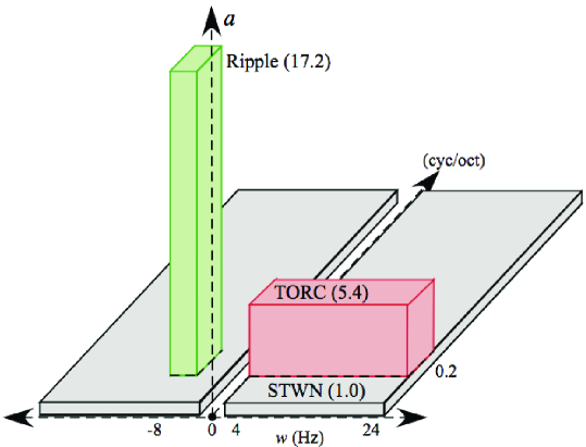
Figure 1: The $S$ magnitudes are illustrated for members of each of the three stimulus types — dynamic-ripple stimuli, TORCs, and STWN. The stimuli all have the same duration ($250$ ms), and contain $1$, $6$, and $90$ spectrotemporal modulation frequencies, respectively. By virtue of the dynamic range constraint on the intensities of the dynamic spectrum, the stimuli must employ different modulation-frequency amplitudes $a$. The amplitudes, relative to those of the STWN stimulus, are indicated in parentheses.

The Fourier series endows dynamic spectra, thus designed, with a common periodicity of $T=250$ ms and $X=5$ octaves. One spectral period was realized in each stimulus, whose $5$-octave bandwidth was centered upon the neuron’s pure-tone tuning curve (measured previously). The temporal periodicity of the dynamic spectra was exploited; this enabled multiple observations of the response, since (assuming the neuron’s memory is less than $T$ seconds) all temporal periods beyond the first constitute identical stimulus presentations. A stimulus sweep consisted of a limited number ($4$ or $12$) of stimulus periods, and had a rise and fall time of $8$ ms. Multiple sweeps were presented for each stimulus. Sweeps of different stimuli, separated by $3$–$4$ seconds of silence, were presented in a pseudorandom order, until a neuron was exposed $60$–$120$ periods ($15$–$30$ s) of each stimulus.

All stimuli were gated and fed through an equalizer into an earphone. Calibration of the sound delivery system (to obtain a flat frequency response up to $20$ kHz) was performed in situ with the use of a $1/8$ in. Brüel & Kjaer 4170 probe microphone. The earphone was inserted into the ear canal through the wall of the speculum to within $5$ mm of the tympanic membrane. The speculum and microphone setup resembles closely that suggested by Evans (Evans,, 1979).

2.2.4 Response Measurement and STRF Calculation

Each stimulus resulted in a collection of response observations ${y[t]}$ (i.e., binned spike trains), each member of which consisted of the number of spikes occurring in successive $\Delta_{t}=1$ ms intervals during one stimulus period (see, e.g., Figure 2B). The total number of stimulus periods used was $n$. The transient epochs, during the first period of each sweep, were disregarded; only the steady-state portion of the response was utilized. The spike rate $r[t]$ was then estimated from the sample mean of $y[t]/\Delta_{t}$: $r[t]={\frac{1}{n}}\sum\limits_{i=1}^{n}{y_{i}[t]/\Delta_{t}}$, where $y_{i}[t]$ is the response to the $i$^th stimulus period. This is the response whose Fourier Transform is used to calculate $H$ (and subsequently the STRF), or some portion thereof, via Eq. (5). These calculations are very simple and are completed in MATLAB (Mathworks) in a fraction of a second.

2.2.5 Reducing Nonlinear Interference with the Inverse-Repeat Method

In this article, we concentrate on even-order nonlinearities; they are ubiquitous in the brain (e.g., due to rectification), and can severely distort the reverse-correlation measurement, particularly when the stimulus is brief (Swerup,, 1978). Fortunately, its ill effects are easily isolated and extracted by the inverse-repeat method (Moller,, 1977; Wickesberg and Geisler,, 1984). In its simplest form, this method calls for two stimuli (here, dynamic spectra) that sum to a constant value. While the linear responses to the two stimuli are opposite in sign, the even-ordered distortion products are identical (Victor and Shapley,, 1980). Therefore, the even-order effects are removed by subtracting the two responses and dividing by two (or instead isolated by adding the responses). This method is investigated in conjunction with TORC stimulation.

2.2.6 Signal and Noise Calculations: Non-systematic Errors

As mentioned in Section 2.1.3, the measures of signal power $P$ and noise variance $\left<\sigma^{2}\right>$, and therefore the SNR, apply to both $h[t,x]$ and $H[w,\Omega]$. For a single stimulus-response pair, a simple relationship was identified in Eq. (6) between the variance of $H[w,\Omega]$ and the variance of $R[w]$. Note that latter variance is, in turn, proportional to the variance of $\tilde{y}[w]$, the Fourier Transform of the response to one stimulus period; specifically,

$$Var\left\{R[w]\right\}={\frac{1}{n}}{\frac{Var\left\{\tilde{y}[w]\right\}}{\Delta_{t}^{2}}}.$$ (8)

Thus, the variance of $H[w,\Omega]$ could be quickly estimated from the sample variance of $\tilde{y}[w]$ (across all stimulus periods), without repeating the experiment or subdividing the data.

However, the $H$ measurement may incorporate the measurements from multiple stimulus-response pairs; if so, its variance will depend on how the individual measurements are combined. If a point on $H[w,\Omega]$ is the average of $N$ measurements, then its variance will simply tend to scale by $1/N$ with respect to that of an individual measurement. But more complicated functions of the individual measurements (such as that used for the dynamic-ripple stimuli (Depireux et al.,, 2001)) may obscure the relation between the variance of $H$ and that of the constituent responses. In such a case, the bootstrap method may be employed. This method simulates the randomness of a statistic that is a function of a collection of identical observations, without repeating the experiment or subdividing the observations (Efron and Tibshirani,, 1993; Politis,, 1998). In the present context, a new $H$ is computed from a new, identical-sized collection of ${y[t]}$, assembled by selecting members of the original collection randomly and with replacement. The sample variance of $H$, or some function thereof, is calculated after repeating the process many times (we used $300$), which is feasible due to the simplicity of the computations.

For the sake of equal footing, we used the bootstrap method to estimate the variance of $H$ for all stimulus types. After subsequently calculating $\left<\sigma^{2}\right>$, the $SNR$ was inferred from the average power of $H$, which, as mentioned in Section 2.1.3, approximately equals $P+\left<\sigma^{2}\right>$.

2.2.7 Signal and Noise Calculations: Systematic Measurement Errors

The SNR quantifies the size of the signal compared to the size of the non-systematic component of the measurement error. However, the possible additional contribution of systematic errors — that is, those induced by non-ideal stimulus structure (i.e., $\tilde{\epsilon}$ in Eq. 4) and by nonlinearities — cause the actual error level of the STRF measurement to exceed that described by the SNR. There exists an opportunity to obtain a more “correct” measure of the SNR, provided that all errors are evenly distributed over the STRF measurement, because the signal tends to be concentrated in an early region of the STRF measurement between $0$ and $125$ ms – in other words, neuron’s responses are only weakly effected by stimulus conditions more than$125$ ms in the past. Accordingly, a corrected SNR measure, $SNR_{cor}$, was obtained after dividing the average power of the early region of the STRF measurement by the average power of the late (post $125$ ms) region. Note that the late region of the STRF measurement contains the uncorrelated contributions of both non-systematic and systematic errors, while the noise power estimate used for $SNR$ only measures the non-systematic component; therefore, $SNR_{cor}$ should be less than or equal to $SNR$ (modulo the inaccuracies in measuring $SNR$ and $SNR_{cor}$), with equality when there are no systematic errors.

2.2.8 Error Reduction with the Singular-Value Decomposition

To further reduce errors in the STRF measurement, we investigated the singular-value decomposition (SVD), applied to either $h[t,x]$ or $H[w,\Omega]$ (which are both just matrices of numbers). The SVD is a well-studied tool for resolving the structure of matrices that are corrupted by errors (Stewart,, 1993; Hansen,, 1998). It works by breaking up an arbitrary matrix into a sum of separable matrices, which, in the current context, are each formed by the product of one temporal vector and one spectral vector. The first matrix takes the best separable approximation out of the original matrix; the second takes the best separable approximation out of the remainder, and so on. The importance of each separable matrix is gauged by its singular value, which is the square root of its average power. The total number of separable matrices required to describe a matrix (the number of nonzero singular values) is called the matrix’s rank.

A basic theorem (Stewart,, 1991) implies that if the error-free STRF can be well approximated by only a few separable matrices, then the addition of small and evenly distributed errors will only slightly perturb their form, as they constitute the first few matrices in the SVD of the STRF measurement. The additional and subsequent matrices required to describe the measurement will describe mostly errors, and thus should be discarded. In fact, there are a priori reasons to believe that STRFs are well approximated by low-rank matrices. Typically, cortical STRFs are localized in a compact area of the spectrotemporal domain and the modulation-frequency domain (Depireux et al.,, 2001; Miller et al.,, 2002); this alone will limit their rank. Still lower limits will be imposed by special structure within the STRF or the $H$, such as spectral-temporal separability (Eggermont et al.,, 1981; Depireux et al.,, 2001; Sen et al.,, 2001), quadrant separability (Depireux et al.,, 2001), and temporal symmetry (Simon et al., subm, ).

In practice, determining which separable matrices should be discarded is a complex problem (Stewart,, 1993; Hansen,, 1998). Most approaches use knowledge or assumptions about the size and structure of the errors to bound the singular values (or functions thereof) of those separable matrices describing mostly errors. Through simulations, we found that methods based solely on variability analysis tended to underestimate the size of the errors; instead, the most generally accurate methods gauged the error level directly from the post-125-ms region of the STRF measurement (for a similar method see (Sen et al.,, 2001)). We used the largest singular value from this region (or its Fourier Transform) to threshold the singular values of the pre-125-ms region (or its Fourier Transform). In theory, the STRF (or $H$) is optimally approximated using only those separable matrices with singular values above this threshold, and discarding the remainder (Stewart,, 1993; Hansen,, 1998).

Although this approximation is in some sense optimal, it is still prone to error. As the error level increases, more and more error leaks into the approximation and, conversely, more and more of the STRF power is lost under the error threshold (Hansen,, 1998). This second case is of primary interest in this study; we will gauge the proportion of (error-free) STRF power excluded from the SVD approximation. A naive gauge of this is $\alpha_{SVD}$, the proportion of the STRF measurement’s power contained in the SVD remainder (Depireux et al.,, 2001). Unfortunately, when the level of measurement error is high, $\alpha_{SVD}$ itself will be inflated, because much of the remainder will consist of error. However, we can use the bootstrap method to estimate the size (average variance) of the part of the remainder resulting from non-systematic errors, and subtract it out. This leads to a more accurate gauge of the proportion of lost STRF power, particularly when the systematic errors are small: $\beta_{SVD}$, the average power of the systematic component of the remainder, divided by $P$. In Section 3.4, we use $\alpha_{SVD}$ and $\beta_{SVD}$ together to study how measurement errors effect the performance of the SVD.

2.2.9 STRF Comparisons

In this article, the correlation coefficient is used to quantify the similarity between two different STRF measurements. This takes values between $-1$ and $+1$, with $+1$ indicating a perfect match. Comparisons are made over the first $125$ ms of the measurements, both before and after the SVD is applied. Note that the correlation coefficients for the pre-SVD comparisons will be limited by $SNR_{cor}$; if two identical STRFs are corrupted by independent and identically distributed errors, the correlation coefficient should approximately equal $SNR_{cor}/(SNR_{cor}+1)$. To the extent that the SVD approximations result in increased SNRs, they will allow for higher correlation coefficients, which we modeled as $gSNR_{cor}/(gSNR_{cor}+1)$, where $g$ represents a multiplicative gain in $SNR_{cor}$.

2.2.10 Simulations

Simulations were employed in order to verify the performance of these methods under realistic conditions. The core of a simulation is an STRF (tailor-made or derived from a low-rank approximation of an actual measurement) and a set of stimuli. The STRF-based responses to the stimuli are computed via Eq. (3). These responses are then altered; usually they are rectified and then subjected to another static nonlinearity, such as a squaring function. The result, representing the time-varying spike rate, is used to create spike trains with inhomogeneous Poisson statistics (Berry and Meister,, 1998; Oram et al.,, 1999), with a time step of $50$ $\mu$s. These spike trains are treated as the responses of a neuron with an unknown STRF, and are subjected to the very same analyses as the real responses. Wherever the bootstrap method was employed, its expected performance was simulated against a Monte-Carlo procedure, employing 300 sets of independent responses with identical spike rates.

3 Results

The results of this study are presented as follows. In Section 3.1, we detail the measurement of a neuron’s STRF using each of the three stimulation types, and we subsequently illustrate the computation of the SVD-based STRF approximations. In Section 3.2, for neurons whose STRFs were measured with multiple stimulus types, we examine the similarity between the multiple measurements and the corresponding SVD approximations, as a function of the level of measurement error. In Section 3.3, we analyze the origins and stimulus dependence of the measurement errors. Finally, in Section 3.4, we study how measurement errors affect the sufficiency of the SVD approximations.

3.1 Overview

In this section, we detail the measurement of a neuron’s STRF using dynamic-ripple stimuli (Figure 2A), TORCs (Figure 2B), and STWN (Figure 2C), respectively. The $S$ magnitudes for examples of each of these stimulus types are illustrated in Figure 1. The respective STRF measurements are denoted STRF_DR, STRF_TORC, and STRF_STWN. Computation of the SVD-based approximations of the measurements is subsequently detailed.

3.1.1 Dynamic-Ripple Stimuli

For the dynamic-ripple stimuli (Kowalski et al., 1996a, ; Depireux et al.,, 2001) shown in Figure 2A, each stimulus is composed of a single spectrotemporal modulation frequency (Fourier component). It can therefore be considered the auditory equivalent to the drifting sinusoidal luminance gratings used in visual neuroscience (Valois and Valois,, 1990). Figure 2A shows the dynamic spectrum of one such stimulus (top panel), which has a temporal modulation rate $w$ of $-8$ Hz and a spectral modulation rate $\Omega$ of $0.2$ cyc/oct.

The response $r[t]$ to this stimulus (middle panel)) exhibits both linear and nonlinear aspects, as well as variability. According to the linear model of Eq. (3), the response should be a pure $8$ Hz sinusoid, with amplitude and phase determined by $H[8,0.2]$. Clearly, $r[t]$ (C: blue) is modulated at $8$ Hz, but it also contains nonlinear components. The (Discrete) Fourier Transform $R[w]$ makes this explicit: In addition to a prominent $8$ Hz component (in red), distortion products (in green) with frequencies of $0$ Hz (the “DC” or average of $r[t]$ over $t$) and $16$ Hz are plainly visible. Given the stimulus composition, these distortion products betray the presence of $2$^nd-order, and possibly $0$^th-order (“spontaneous” activity), nonlinearity (both of which are even-order). With respect to the linear plus DC description (red curve in inset panel), including the $16$ Hz distortion product (black curve) better accounts for the sharpness and non-negative nature of the response.

The remaining portion of the response looks like noise. It is the manifestation of the period-to-period response variability. In the Fourier Transform of the response, it takes the form of a shallow baseline of energy that extends over all frequencies. Note that the square-root of the response variance (i.e., the standard error), calculated via Eq. 8, is similarly distributed over the components of $R[w]$ (black curve).

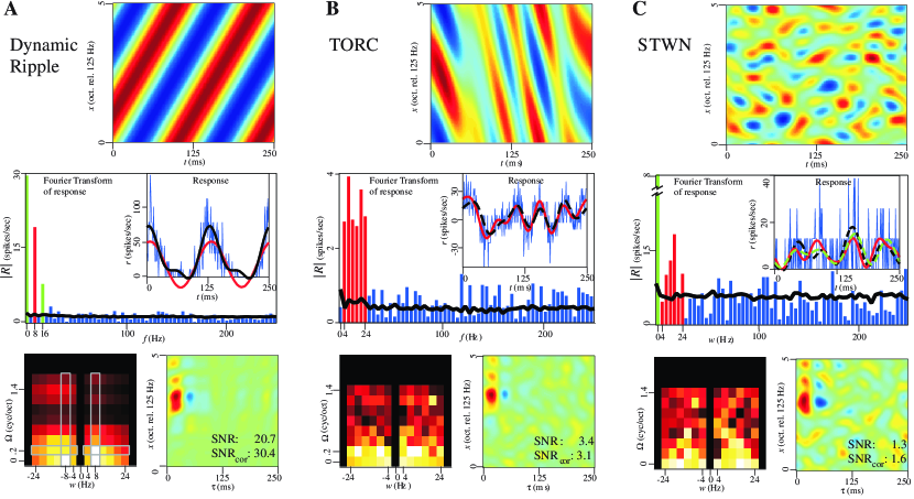
Figure 2: Measuring the STRF of one neuron with different types of ripple stimuli. A: (Top panel) Dynamic spectrum of a single dynamic-ripple stimulus with $w=-8$ Hz and $\Omega=0.2$ cyc/oct. $90$ stimulus periods were used. (Middle panel) Inset displays the response as time-dependent spike rate estimate, $r[t]$: Raw estimate (blue) (using $\Delta_{t}=1$ ms), linear ($8$ Hz) plus DC ($0$ Hz) approximation (red), and the approximation obtained by including the (even-order) $16$ Hz distortion product (black). The magnitude of the Fourier Transform of response is shown in the panel, clearly exhibiting the linear $8$ Hz component (red), nonlinear distortion products (green), and the remaining noise component (blue). Also shown is the square-root of the response variance (the standard error) as a function of frequency (black). (Bottom panels): Measurements of (left) $H$ and (right) $h$ (or STRF_DR) after all $30$ stimuli. The grey outlines in $H$ (left panel) indicate the cross-sections that were directly measured. B: (Top panel) Dynamic spectrum of a TORC with $\Omega=0.2$ cyc/oct and $w$’s between $4$ and $24$ Hz. $75$ stimulus periods were used. (Middle panel) Inset shows response as time-dependent spike rate estimate, $r[t]$, after the inverse-repeat procedure: Raw estimate (blue), linear plus DC approximation (red) obtained by discarding frequencies above $24$ Hz, and the response predicted from the previously obtained STRF_DR in A (dashed black). (Bottom panels): Same as in A above using 15 pairs of TORC stimuli. C: (Top panel) Dynamic spectrum of a STWN with $\Omega$’s between $0.2$ and $1.4$ cyc/oct and $w$’s between $4$ and $24$ Hz. $75$ stimulus periods were used. (Middle panel) Inset shows response as time-dependent spike rate estimate, $r[t]$: Raw estimate (blue), the linear plus DC approximation (red), and the response predicted from STRF_DR (dashed black) and STRF_TORC (dashed green) in A and B above. Panel also shows response Fourier Transform magnitude. The linear $4$–$24$ Hz components (red) are barely distinct from the noise (blue). Also shown is the square-root of the response variance (the standard error) as a function of frequency (black). (Bottom Panels) The measurements of $H$ and STRF_STWN averaged over $30$ stimuli.

The existence of response components due to nonlinearity and variability does not necessarily imply that they interfere with the STRF measurement. Since the stimulus consists of a single spectrotemporal modulation frequency with a temporal component of $8$ Hz, only the $8$ Hz component of the response is correlated with the stimulus, and $\tilde{\epsilon}$ in Eq. (4) is zero. The only source of error is the portion of the nonlinearity and variability that happens to be manifest at $8$ Hz. The reverse-correlation STRF (STRF_DR) can be assembled from results of consecutive presentations of dynamic ripples with different single spectrotemporal modulation frequencies. It is important to note that, due to time constraints, these point-by-point measurements of $H$ were restricted to two cross-sections, as indicated by the gray outlines in left panel (Bottom row). The full $H$ was then constructed from a normalized outer product of these cross-sections (Depireux et al.,, 2001).

3.1.2 Temporally Orthogonal Ripple Combinations

In contrast to the dynamic-ripple stimuli, the TORC stimuli (Klein et al.,, 2000) can directly measure the entirety of the $H$, because each stimulus is used to measure multiple points at once. The stimuli are necessarily more complex, containing six spectrotemporal modulation frequencies (Fourier components) each. However, no two Fourier components in a given stimulus share the same value of $|w|$ (they are temporally orthogonal; their temporal correlation is zero); therefore, each spectrotemporal modulation frequency in the stimulus will evoke a different temporal frequency in the linear part of the response.

The dynamic spectrum of one TORC is shown in Figure 2B (top panel). It is composed of six spectrotemporal modulation frequencies having the same $\Omega$ of $0.2$ cyc/oct, but different $w$’s spanning the range of $4$ to $24$ Hz. The associated response (inset in middle panel: blue) exhibits a complex modulation of the spike rate. The smoothed response, obtained by discarding the frequencies above $24$ Hz, is superimposed in red. A more accurate view of the linear part of the response is also shown (in dashed black), which was obtained from the inverse-repeat procedure. It is very similar to the response predicted by STRF_DR (Figure 2A). The Fourier Transform of the response confirms the strong presence of the $4$ to $24$ Hz components (in red) expected from the linear model. However, with respect to the noise baseline, the response is weaker than it was for the above dynamic-ripple stimulus.

In the reverse-correlation operation, the $4$ Hz response component is orthogonal to all stimulus components besides the $4$ Hz component, the $8$ Hz response component is correlated only with the $8$ Hz stimulus component, and so on; $\tilde{\epsilon}$ is again zero. The STRF after all stimuli are presented, are shown in bottom panels. It bears a striking resemblance to STRF_DR, despite the drop in both $SNR$ and $SNR_{cor}$. This indicates that estimates of the neuron’s STRF are robust to changes in the spectrotemporal modulation frequency content of stimuli.

3.1.3 Spectrotemporally White Noise

The spectrotemporally white noise (STWN) is the most complex of the ripple-based stimuli; its $S$ contains all spectrotemporal modulation frequencies (Fourier components) with equal amplitudes and uniformly distributed phases. The typically poor efficacy of such stimuli can be improved somewhat by limiting the $S$ to a relevant range of spectral and temporal modulation frequencies (Klein et al.,, 2000). Figure 2C (top panel) shows the dynamic spectrum of one such stimulus, which contained all $w$’s between $4$ and $24$ Hz and all $\Omega$’s between $0$ and $1.4$ cyc/oct. Although the response shown below (inset of middle panel) is quite a bit weaker than those observed in Figures 2A and B, when smoothed (red) it is still comparable to the linear predictions from both STRF_DR (dashed black) and STRF_TORC (dashed green); this is despite the fact that the $4$ to $24$ Hz response frequencies predicted by the linear model are barely distinct over the noise baseline.

This reverse-correlation scenario differs from that of the other two stimulus types. Each of the linear response frequencies is now the sum effect of multiple Fourier components of the stimulus sharing the same temporal modulation frequency. Every response frequency will in turn be correlated with each of the stimulus components sharing the same temporal modulation frequency. It is therefore not initially clear which stimulus component caused what component of the response; all points on the $H$ corresponding to a given $w$ cannot be distinguished. This ambiguity manifests itself in the form of a large $\tilde{\epsilon}$.

Because $\tilde{\epsilon}$ is dependent upon the (randomly assigned) phases of the $S$, it has an incoherent structure that is distributed over the entire measurement, and its strength can be reduced by averaging the results from multiple stimuli with different phases (or by using more finely spaced $w$’s, i.e., increasing the base stimulus period $T$) (Klein et al.,, 2000). This argument also applies to the manifestations of variability and even-order nonlinearity (some odd-order distortion products are however not dependent on the phases of the stimulus frequencies (Victor and Shapley,, 1980)). The result obtained after averaging the results from $30$ different stimuli is shown in the bottom panels (approximately the same result would be obtained by extending $T$ by a factor of $30$). Despite a further decrease in $SNR$ and $SNR_{cor}$, its similarity to STRF_DR (Figure 2A) and STRF_TORC (2B) is impressive; the STRF of the neuron has maintained its form for more than an hour, over vastly different stimulus types.

3.1.4 Application of the Singular-Value Decomposition

In this section, we demonstrate the use of the SVD for producing approximations of the measurements of the STRF and $H$. Such approximations represent an optimal trade-off between error reduction and signal loss, provided the errors are evenly distributed over the measurements (Stewart,, 1993; Hansen,, 1998). The proportion of signal lost is gauged by $\beta_{SVD}$ (see Methods).

The SVD of the STRF_TORC from Figure 2B is illustrated again in Figure 3A. The singular values of the first $12$ separable matrices from the SVD are shown (top row), along with the error-derived threshold (see Methods) indicated by the dashed line. The first singular value, corresponding to the separable rank 1 matrix (bottom row), towers over the others, and alone exceeds the threshold. The STRF is well described by this separable matrix, while the sum of the remaining separable matrices, consists of unstructured measurement errors. Indeed, $\beta_{SVD}=4.8\%$, indicating that more than $95\%$ of the STRF power is captured by this rank-$1$ approximation. That is, in large part this STRF represents the product of independent spectral and temporal integration.

In contrast, the SVD of a different neuron’s STRF_TORC is shown in Figures 3B. This STRF does not look separable; for inputs at different tonotopic locations $x$, the temporal integration by the neuron (in its network) is not related by a simple scaling of the same function. In this case, the second singular value (top row panel) also protrudes above the threshold, the rank-$1$ approximation (middle panels) fails to describe the STRF’s obliqueness, and $\beta_{SVD}$ is high at $28.2\%$. After including the second separable matrix (bottom row panels), the approximation is vastly improved ($\beta_{SVD}=6.7\%$), and the remainder again chiefly consists of unstructured errors.

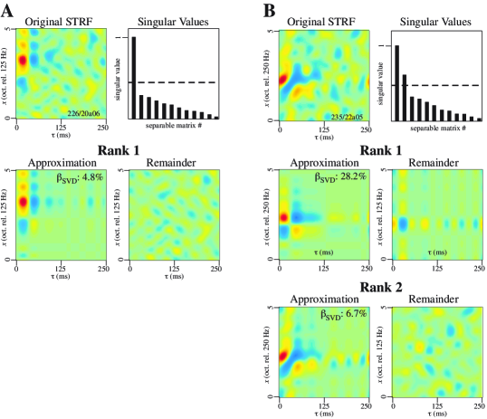
Figure 3: Approximating the STRF with the SVD. A: An STRF that looks separable. (Top row) The original measurement, and the corresponding singular values (bars) of the separable matrices of the SVD, and the error-derived threshold (dashed line). (Bottom row) The rank-$1$ approximation and the remainder. B: An STRF that does not look separable. (Top row) The original STRF and its corresponding singular values (bars) and threshold (dashed line). (Middle row) The rank-$1$ approximation and second-separable matrix (or remainder). (Bottom row) The rank-$2$ approximation, and the remainder. A common color scale is shared by all panels within A, and a different color scale is shared by all panels within B.

The SVD can alternatively be applied to the $H$. While the SVD of the full $H$ yields an approximation identical to that of the STRF, applying the SVD separately to each of the quadrants of the $H$ will generally produce a different approximation. This procedure is of interest chiefly because previous studies (using dynamic-ripple stimulation) have suggested that the $H$’s of AI neurons are well described as being quadrant-separable (Kowalski et al., 1996b, ; Depireux et al.,, 2001), implying that the SVD of each quadrant of the $H$ should yield at most one separable matrix of significance. Therefore, if the STRF is not separable, it could be advantageous (in terms of error reduction) to approximate the STRF in this manner. This principle is examined in Figure 4, using the non-separable STRF from Figure 3B. The SVD of each of the upper two quadrants of the $H$ shown in 4A (middle panel) yields the two sets of singular values (bottom panel). In each quadrant, only the first singular value is pronounced and exceeds the threshold. This indication that the quadrants are indeed separable is supported upon comparison of the original STRF (top panel) with the quadrant-separable approximation (for which $\beta_{SVD}=6.6\%$) and the remainder, shown in B. Intriguingly, the result is markedly similar to the rank-$2$ approximation of the STRF from Figure 3B. By implication, the $H$ from the rank-$2$ approximation (shown in D) is very similar that from the quadrant-separable approximation (in C). The Fourier Transforms of the corresponding remainders are also very similar.

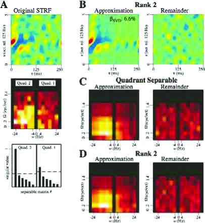
Figure 4: Approximating the $H$ with the SVD. A: (Top panel) The original STRF measurement and (Middle panel)the corresponding $H$ magnitude (first two quadrants). (Bottom panel) The singular values (bars) and thresholds (dashed lines) of the first two quadrants of the $H$. B: The quadrant-separable approximation of the STRF in A and the remainder. C: The $H$ magnitude from the quadrant-separable approximation, and the Fourier Transform of the remainder. D: The $H$ magnitude from the rank-$2$ approximation (from Figure 3), and the Fourier Transform of the remainder (from 3) A common color scale is shared by B and the top panel of A . A different color scale is shared by C, D, and the middle panel of A.

In summary, we have demonstrated the use of the SVD for producing relatively error-free approximations of the STRF or $H$ measurements. Later, in Section 3.4, we will examine how well these three types of approximations — the rank-$1$, rank-$2$, and quadrant-separable approximations — apply to the whole of the neuronal population, as a function of the error level and the type of stimulation.

3.2 Direct Comparisons of STRFs Measured with Different Stimulus Types

In $45$ out of $308$ neurons whose STRFs we measured, we obtained multiple STRF measurements using two or all three stimulus types. The resemblance between the first $125$ ms of each pair of measurements was quantified by the correlation coefficient (see Methods), which was computed under four conditions: for the raw (pre-SVD) measurements, and for the quadrant-separable, rank-$2$, and rank-$1$ approximations of the measurements.

The correlation coefficients from the raw comparisons are plotted in Figure 5A versus the limiting (minimum) $SNR_{cor}$ of the two measurements. The squares, triangles, and circles correspond to the three possible pairs of stimulus types compared. The trends followed by all stimulus comparisons are similar. When $SNR_{cor}$ is above $1$, the correlation coefficients are high and are weakly affected by $SNR_{cor}$. The correlation coefficients are only small when $SNR_{cor}$ is small; as $SNR_{cor}$ descends to $0$, so do the correlation coefficients. This mirrors the relationship expected from two identical STRFs that are corrupted by independent errors, as indicated by the solid-black Curve 1. In other words, it the relationship produced when the STRFs of the system, summarized by the (error-free) STRF, is impervious to changes in stimulus type, but the STRF measurement is error-prone.

Since the SVD approximations act to reduce errors, they should result in higher correlation coefficients, provided the STRF measurements have similar signal components. These properties are evident in the three dashed curves in 5A, which summarize the correlation coefficients obtained from the quadrant-separable (Curve 2), rank-$2$ (Curve 3), and rank-$1$ (Curve 4) approximations of each pair of measurements (the data points are not shown, for clarity). The curves fit the combined data from all three types of stimulus comparisons. The fits were produced by modeling the error reduction as a multiplicative gain $g$ in $SNR_{cor}$ (see Methods). The values of $g$ used for Curves $2$–$4$ are $1.7$, $1.9$, and $2.9$, respectively; these values minimized the number of data points deviating more than $0.1$ units away from the curves (providing the most visually pleasing fits).

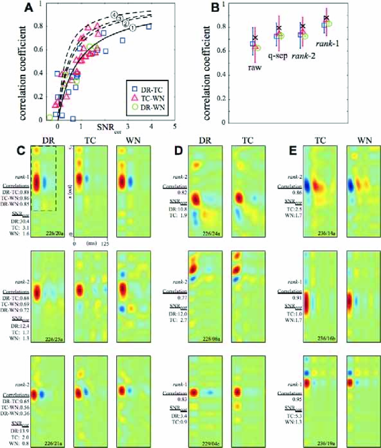
Figure 5: Similarity between STRFs measured with different stimulus types: Dynamic ripple (DR), TORC (TC) and STWN (WN). DR-TC, e.g., denotes comparisons between DR and TORC STRFs. Correlation coefficients were computed between the original (raw) measurements, and between the quadrant-separable (q-sep), rank-$2$ and rank-$1$ approximations of each measurement. A: Correlation coefficients plotted versus minimum $SNR_{cor}$ of the two original measurements. Squares, triangles, and circles correspond to the raw comparisons; different symbols correspond to the different pairs of stimulus types compared (see legend). Curve 1 (solid black) is the relationship expected from two identical STRFs with independent errors. Curves 2, 3, and 4 (dashed curves) are fits to the correlation coefficients obtained from the quadrant-separable, rank-$2$, and rank-$1$ approximations of each measurement, respectively (see text). B: The complete range (vertical lines) and the average (squares, triangles, and circles) of the correlation coefficients are shown for all comparisons where the minimum $SNR_{cor}$ was above $1$. Also shown (black x’s) are the average correlation coefficients, for all pairs of stimulus comparisons combined, obtained when the comparison is further limited to the half-sized rectangular region of the STRF containing the most power (see, e.g., dashed box on the top left STRF of Column C). Columns C, D, E: In each row, the STRF of the same neuron measured with different stimulus types are shown side by side. Shown are either the rank-$1$ or rank-$2$ approximations of the STRFs, depending on what was optimal for the measurement with the highest $SNR_{cor}$. To the left are correlation coefficients obtained from each pair of comparisons and the $SNR_{cor}$ of the original measurements.

For all data points exceeding the critical $SNR_{cor}=1$ level, Figure 5B shows the complete range and the average of the correlation coefficients. Again, similar results are obtained no matter which two stimulus types are compared. For the raw measurements, correlation coefficients fall between $0.5$ and $0.8$, with an average of $0.64$. The average rises to $0.73$ and $0.75$ for the quadrant-separable and rank-$2$ approximations, respectively. For the rank-$1$ approximations, the correlation is $0.85$ on average, is as high as $0.97$, and does not fall below $0.74$. The average correlations are still higher ($0.71$, $0.78$, $0.80$, and $0.88$, respectively) when the comparisons are further restricted to the half-sized rectangular region containing the most power (e.g., the dashed box in the top row of 5C), as indicated by the x’s. Least affected are the rank-$1$ comparisons, suggesting that they are already relatively error free. Note that these values far surpass those typically produced by comparing the STRFs of different neurons; for example, if the rank-$1$ approximation of a neuron’s STRF_TORC was compared to the rank-$1$ approximation of the subsequent neuron’s STRF_STWN, the average correlation was $0.03$.

Some visual comparisons of STRF measurements are available in Columns C through E of Figure 5. For each comparison, either the rank-$1$ or rank-$2$ approximations are shown, depending on what was optimal for the STRF with the highest $SNR_{cor}$. In C are results from three neurons that were tested with all three stimulus types. A typical rank-$1$ result is shown in the top row. The STRFs match in many details, including the suppressive areas and the multiple excitatory areas. In the middle row is a rank-$2$ example with somewhat lower-than-average correlation coefficients. While some features match well across stimuli, there is an increase in background fluctuations between STRF_DR and STRF_STWN that limits the comparisons. The rank-$1$ approximations may have been more appropriate here (and these yielded correlation coefficients over $0.8$). In the bottom row is an unusual rank-$2$ example, where the $STRF$ peak shifts to a higher frequency, thus diminishing the correlation coefficients. However, $SNR_{cor}$ of the STRF_STWN was only $0.8$, so it is difficult to make definite claims about its structure. Results from additional neurons that were tested with two of the three stimulus types are provided in D and E. Overall, a wide variety of STRFs shapes, including unusual “offset” types (E, top row), are well preserved across stimulus type. To be sure, there is much less variation in STRF shape across stimulus type than there is across neurons.

In summary, both visual and quantitative comparisons reveal a close resemblance between the STRFs measured with different stimulus types. The resemblance predictably increases as the limiting $SNR_{cor}$ of the measurements increases; similarly, using the SVD to reduce the error level only serves to increase their resemblance. The highest correlation coefficients result from the rank-$1$ approximations, indicating that they are the most error-tolerant. Similar results are obtained no matter which of the three possible pairs of stimulus types are compared. By the same token, a wide variety of STRFs are observed across neurons.

Together, these observations indicate that linear spectrotemporal processing is a robust property of AI that takes diverse forms in individual neurons.

3.3 The Sources and Stimulus Dependence of Measurement Error

In Section 3.2, it was shown that the signal component of the STRF measurement, seen through the corrective lens of the SVD, is not crucially dependent on the stimulus type. Instead, the ability of the SVD to separate this signal from the measurement errors is crucially dependent on $SNR_{cor}$, which may depend on the stimulus type. In this section, we examine the sources contributing to $SNR_{cor}$ and their stimulus dependence.

3.3.1 Systematic Error

The capacity of systematic errors to limit the quality of the measurements is evident in the relationship between $SNR$ and $SNR_{cor}$. This relationship, observed over all measurements for each stimulus type, is plotted in Figure 6 (with second-degree polynomial fits where appropriate). For both the TORC (A; F, Curve 1) and the STWN (D; F, Curve 4) measurements, $SNR_{cor}$ shows a clear saturating characteristic as $SNR$ increases. Recall that $SNR_{cor}$ incorporates both the non-systematic and systematic errors, while the SNR incorporates only the non-systematic errors. Therefore, as the measurements become more reliable (SNR increases), the saturation of $SNR_{cor}$ evinces the systematic error that dominates when the non-systematic errors are sufficiently small. The relative significance of the systematic error component is revealed in the level to which $SNR_{cor}$ is limited in the high SNR measurements.

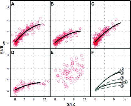
Figure 6: The relationship between $SNR$ and $SNR_{cor}$ across all measurements for each stimulus type, and second-degree polynomial fits (black curves) when appropriate. The level of saturation of these curves indicates the relative levels of systematic errors in the measurements. A: TORC. B: TORC without inverse-repeat, thus retaining systematic errors due to even-order nonlinearities. C: TORC control, discarding half of the stimulus presentations, D: STWN. E: Dynamic ripple. F: Comparison of polynomial fits: Curves 1–4 are from Figures A–D. Curve 5: STWN, discarding half of the stimuli, thus increasing systematic errors induced by the stimulus ($\tilde{\epsilon}$). Curve 6: STWN control, discarding half of the stimulus presentations.

Recall that for the TORC measurements (A; F, Curve 1), the inverse-repeat method was employed in order to remove systematic errors due to even-order nonlinearities. Therefore, the saturation of $SNR_{cor}$ in the TORC measurements should be worsened if the inverse-repeat method is not used. Indeed, bypassing the inverse-repeat method did further limit $SNR_{cor}$ (B; F, Curve 2), by a factor of about $2.5$. Note that this is not simply a side effect of $SNR$ reductions caused by discarding half of the data, for it is not observed if half of the stimulus presentations are discarded but inverse-repeat is still employed (C; F, Curve 3).

In the STWN measurements (D; F, Curve 4), the systematic errors are much more severe than in the TORC measurements; the limiting value of $SNR_{cor}$ is at least $4$ times lower, and so $SNR_{cor}$ is much less likely to exceed usable values. $SNR_{cor}$ is also less variable across the high-SNR measurements; when the measurements are reliable, which is fairly often, $SNR_{cor}$ reliably reaches its limited potential. This potential is further cut in half by discarding half of the stimuli (F, Curve 5), but not by discarding half of the presentations of each stimulus (Curve 6). In sum, these observations suggest that the errors are dominated by the nonideality of the STWN stimuli (i.e., $\tilde{\epsilon}$), to which all neurons were exposed. Our simulations also supported this view. Therefore, at least $4$ times as many STWN stimuli would have to be used in order to raise the $SNR_{cor}$ potential to the level of the TORC method.

Finally, note that the relationship between $SNR$ and $SNR_{cor}$ is less clearly defined in the dynamic-ripple measurements (E) (although both $SNR_{cor}$ and $SNR$ often surpass the values achieved by the other two stimulus types). In our experience, this is largely because the errors are not uniformly distributed over the dynamic-ripple STRFs (Depireux et al.,, 2001), due to the outer-product operation in the construction of the $H$. As a result, $SNR_{cor}$ is a less reliable gauge of the overall error level in the dynamic-ripple measurements.

3.3.2 Non-Systematic Error

In Section 3.3.1, it was shown how the potential accuracy of the STRF measurements is limited by the level of systematic error, which depended on the stimulation method. However, if a method is to achieve a given level of accuracy within its potential, it is evident in Figure 6 that the SNR (which reflects the level of non-systematic error) must be at least minimally adequate. In this section, we explore how the SNR is determined from the interplay between the stimulus, the STRF, and the neuronal response.

To set the stage, recall from Eq. (5) that a single stimulus-response pair results in the measurement of a set of one or more points on $H[w,\Omega]$, which is given by the spectrotemporal modulation frequencies content of the stimulus. By Eq. (6), the variance of each point $(w,\Omega)$ is a fixed proportion, namely $1/a^{2}$, of the variance of the response’s Fourier Transform at the corresponding (temporal) frequency $w$ ($a^{2}$ is the power of each of the spectrotemporal modulation frequencies in the stimulus). Now, consider the whole of the $H$ measurement, built stimulus-by-stimulus. To simplify matters, we will first consider the situation in which every point of the measurement has resulted from a single stimulus-response pair — that is, prior to the TORC inverse-repeat procedure, the STWN phase-averaging procedure, or the dynamic-ripple outer-product operation. In that case, to find the variance of any point on the $H$, one needs only to find the variance of the appropriate response at the appropriate frequency, and weight it by $1/a^{2}$. Consequently, the average variance of the entire $H$ (and STRF) measurement, $\left<\sigma^{2}\right>$, is simply $1/a^{2}$ times the average variance at all of the relevant frequencies of all responses. The SNR is then the ratio of $P$ (the STRF signal power) to this number.

What determines the variance of a response’s Fourier Transform? Two observations lead to a simple answer. First, as middle panels in Figures 2A, 2B, and 2C typify, the variance of $R[w]$ is nearly frequency-invariant (deviations from this could reflect refractoriness, burstiness, or oscillations in the response (Bair and Koch,, 1996)). Therefore, the average variance over the relevant frequencies is closely related to the average variance over all frequencies. Now, the average variance over all frequencies equals the average variance over all times (Papoulis,, 1962; Oppenheim and Schafer,, 1989), which ties in the second observation: The variance of $r[t]$ is proportional to $r[t]/n$ (where $n$ is the number of stimulus periods). This originates from a linear relationship between the sample mean and the sample variance of the binned spike train responses ($y[t]$), which is a widely reported observation (Shadlen and Newsome,, 1998). Consequently, the average variance over time is proportional to the average spike rate over time, $\bar{r}$. So finally, all else being equal across stimuli, $\bar{r}$ (over all responses) can be treated as the lone variable determining the average variance of the responses over the relevant frequencies. The relationship observed across all STRF measurements is shown in Figure 7A, where the variance has been transformed into the variance of a single response period by multiplying by $n$ (thus correcting for differences in $n$ across measurements). The trend across all neurons is indeed linear (on this log-log plot, the slopes of the linear fits to the data were very close to $1$), and is only weakly influenced by stimulus type.

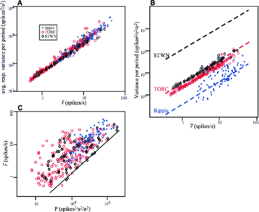
Figure 7: The sources and stimulus dependence of $SNR$, for the dynamic ripple stimuli (blue dots), TORCs (red circles), and STWN (black diamonds). A: The linear relationship between the average spike rate $\bar{r}$ and the average variance of the response’s Fourier Transform. $\bar{r}$ is averaged over all responses. The variance is averaged over all responses, but only those temporal frequencies of each response relevant to the $H$ measurement (where the corresponding $S$ magnitude was nonzero, e.g., $w=4,8,,24$ Hz). The variance is scaled by $n$ (the number of stimulus periods) to correct for differences $n$ across the measurements, and thus represents the variance of a single response period. B: (dashed lines) The expected relationships between $\bar{r}$ and $\left<\sigma^{2}\right>$ (scaled by $n$) in the case where each point of the $H$’s is obtained from a single stimulus-response pair. The actual relationships observed (plotted points) differ from the dashed lines by an amount predicted by the number of stimulus-response pairs whose results are averaged to obtain the final $H$ (see text). C: The lower bound of $\bar{r}$ is proportional to the square-root of the STRF signal power $P$ (the diagonal line’s slope is $1/2$). The square-root law is expected from a linear-plus-rectification response model, but the scatter in $\bar{r}$ suggests additional sources of variability.

In contrast, the choice of stimulus type effects order-of-magnitude differences in $a^{2}$ (due to differences in the number of spectrotemporal modulation frequencies per stimulus; recall Figure 1). This in turn strongly effects the STRF variance $\left<\sigma^{2}\right>$ for a given average spike rate $\bar{r}$. Given the relationship observed between $\bar{r}$ and average response variance in 7A, the predicted relationship between $\bar{r}$ and $\left<\sigma^{2}\right>$ (again scaled by $n$) for each of stimulus type is indicated by the dashed lines in B. Note, however, that for a given neuron, the actual effect of stimulus type on $\left<\sigma^{2}\right>$ depends on how $\bar{r}$ is also affected. Curiously, we have seen little evidence for a significant effect of stimulus type on $\bar{r}$. From one type to the next, up to factor-of-two increases or reductions in $\bar{r}$ were typical, but this variation is not systematic and is small compared that of $a^{2}$.

The actual relationship between the average spike rate and the STRF variance observed across all STRF measurements is indicated by the data points plotted in B. The discrepancies between these trends and the dashed lines, where they exist, are easily explained by the fact that every point of the actual $H$ measurements is not the result of just one stimulus-response pair, as we have so far assumed. For the STWN stimuli, $H[w,\Omega]$ was the average result from $30$ stimulus-response pairs; therefore, its actual variance $\left<\sigma^{2}\right>$ (black diamonds) was lower than the black (upper-most) dashed line by a factor of $30$. This largely compensated for the difference in $a^{2}$ between the STWN and TORC stimuli. Similarly, the inverse-repeat method effectively averages the results from two sets of stimuli, and so the $\left<\sigma^{2}\right>$ of the final TORC result (red circles), was cut in half with respect to the red (middle) dashed line. Finally, we observed that the $\left<\sigma^{2}\right>$ of the final dynamic-ripple $H$ (blue dots), each point of which results from the normalized product of two individual measurements, was typically similar to that of the measured cross-sections alone. Therefore, its relation to $\bar{r}$ was similar to the black (lower-most) dashed line, albeit with quite a bit of scatter. Overall, these properties conspired to produce $SNR$’s that were, on average, a factor of $5$ lower in the TORC measurements than in the dynamic-ripple measurements, and an additional factor of $2$ lower in the STWN measurements.

For each stimulus type, the average spike rate $\bar{r}$ observed across neurons ranged over roughly two orders of magnitude. Figure 7C shows that the value of $\bar{r}$ is partially predicted by the STRF power $P$, in that $\bar{r}$, and more strictly its lower bound, tends to grow by the square-root of $P$ (the black line on this log-log plot has a slope of $1/2$). A square-root relationship is expected from the linear response model followed by rectification: Generally speaking, STRFs (and $H$’s) with higher magnitudes result in spike rates with proportionally stronger modulations, which, since the spike rate must be positive, result in proportionally higher $\bar{r}$’s; meanwhile, $P$ grows as the square of the STRF magnitudes. Since $\bar{r}$ translates linearly into variance, this implies that STRFs with higher average power $P$, although associated with higher absolute levels of variability, have the potential to achieve higher SNRs; and this potential is realized in those neurons with the lowest $\bar{r}$ allowed for a given $P$. Note that the data from all stimulus types overlap, reinforcing the idea that $\bar{r}$ is not significantly affected by stimulus type.

In summary, the ingredients of $SNR$ are of two largely independent varieties: properties of the stimulus and properties of the auditory system. The key stimulus properties boil down to the power in each spectrotemporal modulation frequency $a^{2}$, to which the SNR is inversely proportional, and the number of stimulus-response pairs used to measure each point of the $H$ (including $n$, the number of periods of each stimulus), to which $SNR$ is proportional. The system properties reduce to the STRF power $P$ and the average spike rate $\bar{r}$, to which the SNR is proportional and inversely proportional, respectively. Furthermore, $\bar{r}$ can be seen as the sum of two positive-valued components. One is proportional to the square-root of $P$, as predicted by a linear-plus-rectification response model. The other not obviously related to the STRF, and represents an additional source of variability that varies in strength from neuron to neuron. The net result is that an increase in $P$ serves to increase the SNR, while, for a given $P$, an increase $\bar{r}$ counteracts this effect.

3.4 Sufficiency and Error Dependence of the SVD-Based Approximations

In Section 3.2, the SVD approximations of STRFs measured with different stimulus types were found to be highly similar when $SNR_{cor}$ (which reflects the level of measurement error) was adequate in both measurements. The stimulus dependence of $SNR_{cor}$ was then analyzed in detail in Section 3.3. In this section, we further examine how the SVD approximations are influenced by $SNR_{cor}$. Primarily, we are concerned with the extent to which measurement errors may prevent the SVD from resolving features of the “true” (error-free) STRF.

For this purpose, it would be useful to know the proportion of the true STRF’s power lost from an SVD approximation of the measurement. Unfortunately, in the presence of measurement error, this quantity is not precisely knowable. One way to estimate it is to compute the proportion of the STRF measurement’s power lost from an SVD approximation, which we call $\alpha_{SVD}$ (Depireux et al.,, 2001). In total, we will consider $\alpha_{SVD}^{(1)}$, $\alpha_{SVD}^{(2)}$, and $\alpha_{SVD}^{(QS)}$, which speak to the sufficiency of the rank-$1$, rank-$2$, and quadrant-separable approximations, respectively. One obvious disadvantage of $\alpha_{SVD}$ is that it is inflated in the presence of measurement errors (which comprise much of the measurement’s lost power). This is evident in Figures 8A through C, where $\alpha_{SVD}^{(1)}$ (A), $\alpha_{SVD}^{(2)}$ (B), and $\alpha_{SVD}^{(QS)}$ (C) are plotted versus $SNR_{cor}$ for all TORC and STWN STRFs (recall that $SNR_{cor}$ is unreliable for the dynamic-ripple STRFs). The influence of $SNR_{cor}$ on $\alpha_{SVD}$ clearly persists up to high $SNR_{cor}$’s.

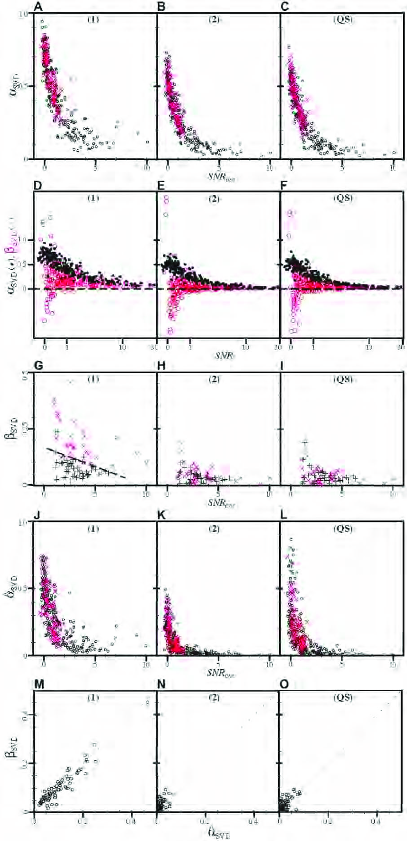
Figure 8: Sufficiency of the SVD approximations as a function of the error level. A–C: $\alpha_{SVD}$, the proportion of the STRF measurement’s power lost from the SVD approximations, for all TORC (black o’s) and STWN (red x’s) measurements. D–F: $\beta_{SVD}$ (red o’s) and $\alpha_{SVD}$ (back dots) versus $SNR$ for all TORC measurements. $\beta_{SVD}$ estimates the proportion of the systematic part of the STRF measurement relegated to the SVD remainder, and therefore better reflects the true STRF’s structure. At very low SNRs, $\beta_{SVD}$ is unstable (some points lay beyond the axis limits). G–I: $\beta_{SVD}$ versus $SNR_{cor}$ for all TORC measurements with $SNR$ above $1.5$. Black +’s and red x’s denote those measurements optimally approximated by rank-$1$ (separable) and rank-$2$ (non-separable) matrices, respectively. With $\beta_{SVD}^{(1)}$ (G) typically as high as $25\%$, many STRFs are not well described by the rank-$1$ approximations. In contrast, $\beta_{SVD}^{(2)}$ (H) and $\beta_{SVD}^{(QS)}$ (I) are typically well below $10\%$, indicating that all STRFs are well described by both the rank-$2$ and quadrant-separable approximations. The unusually high $\beta_{SVD}$’s at the lowest $SNR_{cor}$’s indicates that the SVD is unable to resolve the structure of some non-separable STRFs with high error levels. J–L: $\hat{\alpha}_{SVD}$, computed as $\alpha_{SVD}$ but from the quadrant-separable (J, K) and the rank-$2$ (L) approximations of the TORC (black o’s) and STWN (red x’s) measurements. M–O: As expected, the $\hat{\alpha}_{SVD}$’s are well matched to the corresponding to $\beta_{SVD}$’s in those TORC measurements with $SNR_{cor}$ above $2$.

We reduced the dependence of $\alpha_{SVD}$ on the error level by removing the effect of the non-systematic errors (see Methods). The improved measure, $\beta_{SVD}$ is a more accurate gauge of the proportion of lost STRF power, especially when the systematic errors are small (e.g., in the TORC measurements). In theory, $\beta_{SVD}$ should be more tolerant than $\alpha_{SVD}$ to changes in SNR, and $\alpha_{SVD}$ should converge down to $\beta_{SVD}$ with increasing $SNR$. These properties are verified in Figures 8D through F, where $\beta_{SVD}$ (red circles) and $\alpha_{SVD}$ (back dots) are plotted versus $SNR$ for the TORC measurements (the only caveat is that at very low SNRs, $\beta_{SVD}$ becomes unstable). It is concluded (with additional support from our simulations) that at moderate to high $SNR$s, the effect of non-systematic error is accurately removed in the computation of $\beta_{SVD}$. Therefore, $\beta_{SVD}$ estimates the proportion of the systematic part of the STRF measurement relegated to the SVD remainder, and better reflects the true STRF’s structure. To be conservative, we will consider $\beta_{SVD}$ only in those measurements with $SNR$’s over $1.5$.

The relationship between $\beta_{SVD}$ and $SNR_{cor}$ for the $82$ TORC measurements meeting this criterion is plotted in Figures 8G through I. The blue +’s and red x’s denote the $50$ and $31$ measurements optimally approximated by rank-$1$ and rank-$2$ matrices, respectively (the lone rank-$3$ approximation is not shown). At moderate to high $SNR_{cor}$’s (e.g., above $2$), the $\beta_{SVD}$ distributions are only weakly dependent on $SNR_{cor}$. In other words, the SVD approximations are only weakly affected by measurement errors, and therefore $\beta_{SVD}$ should more accurately reflect the structure of the true STRF. Therefore, the typical range of $\beta_{SVD}^{(1)}$ (8G), roughly from $3\%$ to $25\%$, indicates many STRFs are poorly described by rank-$1$ approximations. It is reassuring that the lower and upper portions of this range are dominated by the measurements optimally approximated by rank-$1$ and rank-$2$ matrices, respectively. However, the boundary between the two populations progressively shifts from about $5\%$ at the highest $SNR_{cor}$ to nearly $15\%$ at the lowest $SNR_{cor}$. This reflects the fact that the optimal trade-off between error reduction and signal loss afforded by the SVD approximations gets worse as $SNR_{cor}$ decreases; at higher error levels, the true STRF must be further from being rank-$1$ before the second separable matrix of the SVD becomes dominantly signal and is included in the approximation.

Over this same range of suitably high $SNR_{cor}$’s, $\beta_{SVD}^{(2)}$ (H) and $\beta_{SVD}^{(QS)}$ (I) are universally bound below $10\%$, with averages of $3.1\%$ and $3.6\%$, respectively. That is, the true STRFs are almost completely contained within both the rank-$2$ and quadrant-separable approximations of TORC measurements with suitably low error levels. Indeed, as was illustrated in Section 3.1.4, the two approximations were usually very similar.

When $SNR_{cor}$ is low, a handful of measurements have conspicuously high values of $\beta_{SVD}^{(1)}$ (G), $\beta_{SVD}^{(2)}$ (H), or $\beta_{SVD}^{(QS)}$ (I). There are three plausible reasons for this: (1) The systematic errors in these measurements are unusually large (thus inflating $\beta_{SVD}$); (2) The true STRFs are actually poorly described by these SVD approximations, and coincidentally the measurements have a high error level; (3) Because of the high error level, the SVD of these STRFs shapes is being disrupted, and more STRF power is being lost than otherwise would be. We favor the last reason, since (despite the error level) most of these STRFs appear to have non-separable shapes. Such STRFs are are also found at higher $SNR_{cor}$’s, but these high values of $\beta_{SVD}^{(2)}$ and $\beta_{SVD}^{(QS)}$ are not found at higher $SNR_{cor}$’s.

Although they are needed to fully describe many STRFs, the trade-off to using the rank-$2$ or quadrant-separable approximations instead of the rank-$1$ approximations is that they retain a higher proportion of the measurement error. This was earlier indicated in Figures 5A and B. Similarly, for the these TORC measurements, we estimated (using the bootstrap method) that the SNR of the rank-$1$ approximation is on average $3.4\pm 0.6$ times higher than that of the raw measurement, while for the rank-$2$ and quadrant-separable approximations, the average gain in $SNR$ is reduced to $2.0\pm 0.6$ and $1.9\pm 0.6$, respectively. Note that these values are comparable to the $SNR_{cor}$ gain values $g$ employed in Section 3.2. Although the rank-$1$ approximations have higher SNRs, which means that they remove proportionally more noise than signal from the measurements, the proportion of signal removed (as gauged by $\beta_{SVD}$) is unacceptably high for many STRFs.

In order to cross-check the results obtained from $\beta_{SVD}$, we recomputed $\alpha_{SVD}$ from the SVD approximations (denoted by $\hat{\alpha}_{SVD}$), rather than from the raw measurements. For example, if the quadrant-separable approximation is indeed a complete and relatively error-free version of the true STRF, then computing $\hat{\alpha}_{SVD}^{(1)}$ and $\hat{\alpha}_{SVD}^{(2)}$ from it should yield results close to the corresponding $\beta_{SVD}^{(1)}$ and $\beta_{SVD}^{(2)}$ (from the raw STRF measurement). Similarly, computing $\hat{\alpha}_{SVD}^{(QS)}$ from the the rank-$2$ approximation should yield a result close to $\beta_{SVD}^{(QS)}$. These $\hat{\alpha}_{SVD}$’s are plotted in Figures 8J through L versus $SNR_{cor}$ for both the TORC and STWN measurements. With respect to the original $\alpha_{SVD}$’s in 8A through C, they are more tolerant to changes in $SNR_{cor}$ over a wider range of $SNR_{cor}$’s. When $SNR_{cor}$ is above $2$, these $\hat{\alpha}_{SVD}$’s are indeed closely matched to the corresponding $\beta_{SVD}$’s, as Figures 8M through O attest. When $SNR_{cor}$ drops below $1$, the $\hat{\alpha}_{SVD}$’s rapidly increase and lose their correspondence with $\beta_{SVD}$, presumably because the assumption that the SVD approximations are complete and error-free rapidly breaks down.

In this section, we have concentrated on the TORC measurements. They are ideal in that they produced low levels of systematic error and a wide range of $SNR_{cor}$’s. The STWN measurements were less than ideal in that $SNR_{cor}$ was limited below $2$. In Section 3.3.1, this was found to be chiefly due to high levels of stimulus-induced systematic error; indeed $\beta_{SVD}$ was grossly inflated in these measurements, rendering it no more illuminating than $\alpha_{SVD}$ (not shown). Nevertheless, over the range of $SNR_{cor}$ that they can be compared, the distributions of $\alpha_{SVD}$ in Figures 8A through C and $\hat{\alpha}_{SVD}$ in J through L were very similar for the STWN and TORC measurements. Moreover, from Section 3.2, the SVD approximations of STWN and TORC measurements were increasingly well matched as the error level dropped. Therefore, the available evidence supports the hypothesis that, for a given level of measurement error, the STWN results and TORC results are equivalent, but the STWN results are much more error prone. The dynamic-ripple results were less than ideal in that STRF_DR is quadrant-separable by construction. Additionally, it contains non-uniformly distributed errors (Depireux et al.,, 2001), which complicates both the SVD (Stewart,, 1993) and the interpretation of $SNR_{cor}$. With this caveat, we note that the distribution (although not the range) of $\beta_{SVD}^{(1)}$ was skewed toward somewhat higher values in the dynamic-ripple measurements. For instance, $\beta_{SVD}^{(1)}$ exceeded $10\%$ in $61\%$ of STRF_DR’s versus $45\%$ of STRF_TORC’s. Still, $\beta_{SVD}^{(2)}$ was below $5\%$ in $91\%$ of STRF_DR’s; the indications were that most STRF_DR’s were still well described by rank-$2$ approximations.

In summary, the optimal SVD approximation of an STRF measurement with a sufficiently low error level (e.g., $SNR_{cor}$ above $2$) does well describe the STRF, in that it preserves at least $90\%$ of the STRF’s power. Therefore, we can be confident that if the SVD approximations of two STRF measurements are well matched, so are the corresponding STRFs. However, when there exist higher levels of measurement error, this is no longer guaranteed to be the case, particularly for STRFs that contain a significant non-separable component. Overall, around $60\%$ of the TORC measurements were well described as being separable. The rest were better served by both rank-$2$ and quadrant-separable approximations, which were essentially identical. To the extent that they could be compared, the STWN and dynamic-ripple measurements produced similar results.

4 Discussion

A pseudo-random exploration of the space of spectrotemporal patterns, fostered by the traditional methodology of reverse correlation, has been the basis of most previous STRF measurements. Instead, we applied a deterministic and analytical reformulation of reverse correlation, which is based upon the Fourier-series description of dynamic spectra. One advantage of this approach concerns experimental optimization: It enables us to restrict the stimulus space to a minimal, discrete set of spectrotemporal patterns (the spectrotemporal modulation frequencies, presented simultaneously or individually). It also facilitates our understanding of measurement errors and their various stimulus- and response-induced components. In sum, it enables us to design stimuli that are efficient and effective, while taking into account general knowledge of the STRF structure, response nonlinearity and variability, and specific laboratory constraints. A second advantage concerns experimental evaluation: Since any given dynamic spectrum can be described by its Fourier series, we can understand and quantify the performance of different stimulation methods, even if they were devised within different frameworks. Both of these advantages have been demonstrated in this study, where we have measured STRFs of AI neurons with three very different types of stimuli.

We now discuss the major empirical results of this study.

4.1 Linearity

The most striking finding is that when the STRF of an AI neuron is successfully measured with different types of stimuli, the results are very similar. The STRFs themselves exhibit a high degree of richness and diversity across neurons. The three types of stimuli used, Dynamic Ripples, TORCs, and STWN differ greatly in their spectrotemporal characteristics and statistics (c.f. Figures 1, and top panels in 2A,B,C), and indeed they sound quite distinct from one another. Great differences even exist between stimuli of a given type (except for STWNs, which all sound noise-like). That STRFs measured from such widely different stimuli are so similar speaks to the significance and robustness of the linearity of neurons’ responses with respect to the dynamic spectra of stimuli. Strong nonlinear system behavior would almost surely interfere with the STRF measurements, not allowing the STRFs generated from such different stimuli to have such large correlation coefficients (except trivial cases such as static nonlinearities, e.g., rectification). The correlation coefficients are especially large considering that the STRF measurements contain large low-power regions (error-prone even after the SVD), and furthermore compared measurements were often made over an hour apart.

4.2 Efficacy of the stimuli

Although, when successful, they lead to very similar STRF measurements, the three types of stimuli differ in their rates of success. Success is achieved when the STRF measurement contains sufficiently low levels of both non-systematic and systematic errors, reflected by the measures of $SNR$ (using only non-systematic error) and $SNR_{cor}$ (including systematic error). Non-systematic errors, caused by response variability, are reduced when the modulations in the stimulus are more powerful (evoking stronger modulations in the response relative to the average spike rate), and also by averaging the results from stimuli with identical spectrotemporal statistics. Systematic errors, caused when multiple stimulus components evoke interfering response components (either linearly or nonlinearly), are reduced by careful stimulus design, or by averaging the results from stimuli with identical spectrotemporal statistics (but different individual characteristics). Note that all of the stimulus types used had approximately the same total presentation duration.

On balance, the stimuli that gave the best results were TORCs, which benefitted from careful stimulus design and relatively strong responses, due to the restricted number of spectrotemporal modulation frequencies in each stimulus. As a result, we have noted that usable STRF measurements could have been obtained after presenting one sweep of each TORC stimulus (taking about $3$ minutes), a fact that we intend to exploit in the future. STWN, while strongly motivated by the traditional reverse correlation methodology, gave STRFs with substantially more systematic error than TORCs. While both stimuli are capable of giving STRFs with high $SNR$, the STWN results in substantially poorer $SNR_{cor}$. This is most cleanly seen by comparing figure panels 6A and 6D: both stimulus types give STRFs with $SNR$ as high as $30$, but STWN generated STRFs have $SNR_{cor}$ that saturate below $2$, while TORC generated STRFs have $SNR_{cor}$ saturating at substantially higher values.

Although the dynamic-ripple stimuli produce the most reliable results (highest $SNR$), they suffered a fundamental flaw: Too many stimuli were required to measure the full MTF_ST (and hence its STRF), and so measurements were restricted a subset of stimuli required if the MTF_ST is quadrant-separable. This is problematic for two main reasons. First, it makes it impossible to assess the quadrant-separability assumption directly. Although quadrant-separability holds in (ketamine-anesthetized) AI, there may be other neuronal populations or experimental conditions for which it doesn’t. Second, the full MTF_ST measurement is a more complex (nonlinear) function of the individual stimulus-response relationships. This complicates the evaluation of measurement errors, and thus blurs the distinction between neural functionality and methodological artifact. Indeed, the dynamic-ripple results had a few subtle idiosyncrasies, including more non-separable STRFs, and $SNR_{cor}$’s poorly correlated with other assays of measurement errors ($SNR$) and STRF structure ($\alpha_{SVD}$, $\beta_{SVD}$). However, since the measurements are so reliable, it may be feasible to sacrifice some $SNR$ by reducing the number stimulus repetitions in order to present all stimuli required to directly measure the full $H$ (Versnel et al.,, 2002).

Finally, we note that the TORC approach is not limited to the particular stimuli used in this study. Any combination of spectrotemporal modulation frequencies could exist in each stimulus, provided that they are temporally orthogonal. Therefore one can produce “super” TORCs, using fewer (but longer-duration) stimuli, each of which contains many spectrotemporal modulation frequencies (Klein et al.,, 2000). These stimuli are more noise like, but benefit from a lack of stimulus-induced systematic measurement errors in contrast to the STWN stimuli. We are currently investigating the effectiveness of such stimuli.

4.3 The SVD: error reduction and signal loss

In this paper, we used the SVD to reduce errors in the STRF measurements. The SVD is ideally suited for use with the STRFs measured here, because their SVD is strongly dominated by the lowest order terms; that is, they are well approximated by a small number of fully separable (rank-$1$) matrices. When such STRFs are perturbed by unstructured errors, the SVD is still strongly dominated by the lowest order terms, and has a well-understood contribution from higher order terms. The boundary between the low order (high signal, low error) and high order (low signal, high error) terms is not known a priori, but is well understood from signal detection theory. The upshot is that truncating the SVD series of an STRF at low order is an efficient and well-understood way of increasing $SNR$ while minimizing loss of signal.

Of the STRF measurements that were suitably error-free, more than half were not only optimally approximated but well approximated (as reflected by $\beta_{SVD}$) by fully separable (rank-$1$) matrices. These approximations reduced the error power by at least a factor of $3$ while sacrificing less than a tenth of the signal power. The rest of the STRFs required two SVD terms (rank-$2$ approximations); using only one SVD term (rank-$1$) would give an incomplete view of the system functionality due to excessive signal loss. The rank-$2$ approximations have somewhat diminished error reduction, down to a factor of $2$. Alternatively, the quadrants of the MTF_ST could be approximated by fully separable matrices, producing results very similar to the rank-$2$ approximations. However, if the error level was too high (e.g., $SNR_{cor}$ below $1$), the optimal SVD approximations no longer reliably achieved both significant error reduction and adequate signal retention. The error level should always be considered when interpreting the results of the SVD.

4.4 The SVD: functional implications

It is intriguing that STRFs are equally well described by rank-$2$ and quadrant-separable approximations (see Figures 8H and I). These properties, each special in their own right, do not necessarily imply one another. It turns out that if an STRF is both rank-$2$ and quadrant-separable, special phase relationships must exist, in either the temporal or spectral dimensions (or both), between the separable matrices of the SVD or equivalently the quadrants of the MTF_ST. It has been demonstrated (Simon et al., subm, ) that AI STRFs possess this property in the temporal dimension (but not necessarily the spectral). This itself has strong theoretical implications for the network connectivity of those neurons.

4.5 The error measures

We found that incorporating systematic errors (otherwise known as bias) into our consideration of the total measurement error level is absolutely crucial for aligning the results from different types of stimuli, and thus understanding the structure of an STRF measurement (and the resulting SVD approximations, correlation coefficients, etc.) independent of stimulus type. We used and analyzed two different measures of error: $SNR$ and $SNR_{cor}$. $SNR$ is the more classical but more limited of the two; $SNR$ is the ratio of the measured STRF power to the measured STRF variance (square of the standard error). This definition of $SNR$ (and its associated measure of error) is not able to incorporate systematic error, however. In contrast, $SNR_{cor}$ does incorporate systematic error. $SNR_{cor}$ is the ratio of measured STRF power to measured non-STRF power (e.g., the power in the spectrotemporal region where the underlying STRF is expected to have near-zero power).

The only problem with $SNR_{cor}$ is that it requires assumptions about the structure of the errors and the STRF, which may not apply to all STRFs and stimuli. In particular, we assumed (based primarily on observations) that errors are evenly distributed over the measurements, and that the STRF power is near zero for $\tau$ above $125$ ms (using negative $\tau$’s is no different since the stimuli were periodic). The usefulness and predictability of $SNR_{cor}$ demonstrated that these assumptions largely held for the TORC and STWN measurements. This was not the case for the dynamic-ripple measurements, however, likely due to a combination of response nonlinearity and the nonlinearity of the STRF measurement itself, which distributes the errors non-uniformly in the spectrotemporal (and modulation frequency) domain. It will be even more useful in the future to devise measures of the systematic errors that are less dependent on the structure of the STRF measurement.

4.6 Response variability

In our investigation of non-systematic errors in the STRF measurements, several observations concerning the variability of AI responses have interesting functional implications. For example, the fact that the response variance could be linearly predicted from the average spike rate in a nearly stimulus-independent manner points to a Poisson-like spike generation mechanism, which has been vigorously investigated in the visual system (Shadlen and Newsome,, 1998). Additionally, we found (see Figure 7C) that while neurons with higher-power STRFs (higher $P$) tended to fire more spikes (higher $\bar{r}$, as might be expected from a linear-plus-rectification response model), a range of average spike rates were still observed for any given STRF power. Neurons with the lowest spike rates (for a given $P$) corresponded to the highest-SNR STRFs, and had the sharpest, most phase-locked responses of the population (not shown). Neurons with the highest spike rates often had seemingly random responses and poor-quality STRF measurements. We will consider the origins and implications of such behavior more carefully in future studies.

4.7 Related studies

Other recent studies have also addressed the similarity of STRF measurements with different types of stimuli, albeit in different auditory loci. Escabí and Schreiner (Escabí and Schreiner,, 2002) measured STRFs in cat inferior colliculus (IC) with stochastic stimuli that in some respects resemble the dynamic-ripple stimuli and STWN used here. While their results largely agree with ours, they singled out a small group of neurons that either exhibited extremely selective and phase-locked responses to the dynamic-ripple-like stimuli but were unresponsive to the STNW-like stimuli (type-II neurons), or exhibited non-phase-locked nonlinear responses to both stimuli (type-III neurons). As discussed above, in AI we also find that neurons’ responses can be extremely sparse and yet yield significant STRFs (like their type-II neurons). However, we did not observe two distinct populations of neurons; rather, the degree of phase locking in response to all stimuli ranged over a continuum. In addition, some AI neurons exhibited significant spike rates but poor STRF measurements (like their type-III neurons). Although we have not yet found a nonlinear relationship between these responses and the dynamic spectra of the stimuli, we can not yet rule out that possibility. In another study, Theunissen et. al. (Theunissen et al.,, 2000) measured STRFs in the zebra finch auditory forebrain in response to random tone sequences and bird songs, and used the STRF from one stimulus to predict the responses to the other. They found small but significant differences in the cross-predictability of the responses, which was poor overall. These differences either reflect differences in the STRF-measurement method (which was implemented as a nonlinear function of the responses), or more probably reflect a higher degree of nonlinearity in the responses of neurons in the avian auditory forebrain with respect to mammalian AI (but see (Schafer et al.,, 1992), who reported a higher degree of linearity and predictability).

4.8 Nonlinearity

This article has been concerned with nonlinearities only insofar as they interfere with the STRF measurement, and methods were invoked to reduce this interference (e.g., the inverse-repeat method). Other methods are also available, such as more carefully choosing the temporal modulation frequencies in the TORCs, so that the nonlinear distortion products are also orthogonal to the linear response (a la (Victor and Shapley,, 1980)). That is not so say that nonlinearities form an insignificant part of the AI response, merely that linearity is important, strong, and robust to changing stimulus conditions, and therefore forms an sturdy foundation upon which the study of auditory cortical processing can be based, even in its nonlinear aspects.

We are currently investigating several anticipated nonlinearities. These include the nonlinear transformation of responses occurs at the thalamo-cortical depressing synapse, which contributes a rapid adaptation of onset responses towards a steady state within a few tens of milliseconds (Denham,, 2001; Kowalski et al., 1996a, ; Phillips et al.,, 2002; Heil,, 1997) (we considered only the steady-state response in this study). Additionally, we have observed that when stimuli contain both low and high modulation frequencies, AI responses can phase lock to much higher frequencies than previously expected (e.g., $100-200$ Hz) (Elhilali et al.,, 2004). Similar effects have been observed in the visual system (Bair and Koch,, 1996; Reid et al.,, 1992; Chance et al.,, 1998). In our stimuli, these high modulation frequencies result from interactions between unresolved AM tones (that fall within the bandwidth of the same cochlear filter), even though they were not part of the target dynamic spectrum (and therefore did not contribute to the STRF measurement). A third nonlinearity is the potential dependence of responses on the bandwidth of the stimulus. Broadband sustained stimuli (such as the ripples, TORCs, and STWN) likely bias cortical cells in a manner different from that of narrowband or transient stimuli such as tones and clicks. Consequently, predicting details of tone and click responses from the STRF may prove sometimes problematic (Kowalski et al., 1996b, ; Theunissen et al.,, 2000). However, this nonlinearity is irrelevant when the focus is on comparing STRFs derived from similarly broadband and sustained stimuli, as is the case in this paper. Yet another important source of nonlinear effects are static nonlinearities (e.g., rectification, response saturation) with respect to stimulus level and contrast. By fixing stimulus contrast at near maximum ($90\%$), and the absolute level at an intermediate value (e.g., based on the rate-level function (Kowalski et al., 1996b, ) we have managed to obtain reliable reproducible results from a sizable proportion of cells in A1. Finally, there are fundamental nonlinearities that we have not yet convincingly observed in AI responses, such as units analogous to the complex cells of the visual cortex (Valois and Valois,, 1990). Nevertheless, it is likely that a significant proportion of the very low SNR STRFs observed in this study belong to cells that would be classified as nonlinear in that they either phase-lock poorly to our stimuli or respond to more complex patterns that we have not been able to probe (e.g., see (Escabí and Schreiner,, 2002)).

References

- (1) Aertsen, A. and Johannesma, P. (1981a). A comparison of the spectro-temporal sensitivity of auditory neurons to tonal and natural stimuli. Biological Cybernetics, 42:145–156.
- (2) Aertsen, A. and Johannesma, P. (1981b). The spectro-temporal receptive field: A functional characteristic of auditory neurons. Biological Cybernetics, 42:133–143.
- Aertsen et al., (1980) Aertsen, A., Johannesma, P., and Hermes, D. (1980). Spectro-temporal receptive fields of auditory neurons in the grassfrog. II. Analysis of the stimulus-event relation for tonal stimuli. Biological Cybernetics, 38:235–248.
- Atlas and Shamma, (2003) Atlas, L. and Shamma, S. (2003). Joint acoustic and modulation frequency. EURASIP Journal of Appllied Signal Processing, 2003(7):668–675.
- Bair and Koch, (1996) Bair, W. and Koch, C. (1996). Temporal precision of spike trains in extrastriate cortex of the behaving macaque monkey. Neural Comput., 8:1185–1202.
- Berry and Meister, (1998) Berry, M. and Meister, M. (1998). Refractoriness and neural precision. Journal of Neuroscience, 18(6):2200–2211.
- Boyd et al., (1983) Boyd, S., Tang, Y., and Chua, L. (1983). Measuring Volterra kernels. IEEE Transactions on Circuits and Systems, 30:571–577.
- Carandini et al., (2002) Carandini, M., Heeger, D., and Senn, W. (2002). A synaptic explanation of suppression in visual cortex. Journal of Neuroscience, 22(22):10053–10065.
- Chance et al., (1998) Chance, F., Nelson, S., and Abbott, L. (1998). Synaptic depression and the temporal response characteristics of V1 cells. Journal of Neuroscience, 18(12):4785–4799.
- Chi et al., (1999) Chi, T., Gao, Y., Guyton, M. C., Ru, P., and Shamma, S. (1999). Spectro-temporal modulation transfer functions and speech intelligibility. Journal of the Acoustical Society of America, 106(5):2719–32.
- Cohen, (1995) Cohen, L. (1995). Time-Frequency Analysis. Prentice-Hall.
- de Boer and de Jongh, (1978) de Boer, E. and de Jongh, H. (1978). On cochlear encoding: Potentialities and limitations of the reverse-correlation technique. Journal of the Acoustical Society of America, 63:115–135.
- deCharms et al., (1998) deCharms, R., Blake, D., and Merzenich, M. (1998). Optimizing sound features for cortical neurons. Science, 280:1439–1443.
- Denham, (2001) Denham, S. (2001). Cortical synaptic depression and auditory perception. In Greenberg, S. and Slaney, M., editors, Computational Models of Auditory Function, NATO ASI Series, Amsterdam. IOS Press.
- Depireux et al., (2001) Depireux, D. A., Simon, J. Z., Klein, D. J., and Shamma, S. A. (2001). Spectro-temporal response field characterization with dynamic ripples in ferret primary auditory cortex. J Neurophysiol, 85(3):1220–34.
- Efron and Tibshirani, (1993) Efron, B. and Tibshirani, B. (1993). An introduction to the bootstrap. New York: Chapman and Hall.
- Eggermont, (1993) Eggermont, J. (1993). Wiener and Volterra analyses applied to the auditory system. Hearing Research, 66:177–201.
- Eggermont et al., (1981) Eggermont, J., Aertsen, A., Hermes, D., and Johannesma, P. (1981). Spectro-temporal characterization of auditory neurons: Redundant or necessary? Hearing Research, 5:109–121.
- (19) Eggermont, J., Aertsen, A., and Johannesma, P. (1983a). Prediction of the responses of auditory neurons in the midbrain of the grass frog based on the spectro-temporal receptive field. Hearing Research, 10:191–202.
- (20) Eggermont, J., Johannesma, P., and Aertsen, A. (1983b). Reverse-correlation methods in auditory research. Quarterly Review of Biophysics, 16:341–414.
- Elhilali et al., (2004) Elhilali, M., Klein, D., Fritz, J., Simon, J., and Shamma, S. (2004). The enigma of cortical responses: slow yet precise. In Auditory signal processing, psychoacoustics, and models, (in press), New York. Springer Verlag.
- Epping and Eggermont, (1985) Epping, W. and Eggermont, J. (1985). Single-unit characteristics in the auditory midbrain of the immobilized grassfrog. Hearing Research, 18:223–243.
- Escabí and Schreiner, (2002) Escabí, M. A. and Schreiner, C. E. (2002). Nonlinear spectrotemporal sound analysis by neurons in the auditory midbrain. Journal of Neuroscience, 22(10):4114–4131.
- Evans, (1979) Evans, E. F. (1979). Single-unit studies of mammalian cochlear nerve. In Beagley, H. A., editor, Auditory investigations: the scientific and technological basis, volume 68, pages 324–367, Oxford, UK. Clarendon.
- Hansen, (1998) Hansen, P. (1998). Rank-deficient and discrete ill-posed problems. SIAM monographs on mathematical modeling, Philadelphia.
- Heil, (1997) Heil, P. (1997). Auditory cortical onset responses revisited. I. First-spike timing. J.Neurophys., 77:2616–16641.
- Hermes et al., (1981) Hermes, D., Aertsen, A., Johannesma, P., and Eggermont, J. (1981). Spectro-temporal characteristics of single units in the midbrain of the lightly anaesthetised grass frog (Rana temporaria L.) investigated with noise stimuli. Hearing Research, 5:147–178.
- Hermmansky, (1999) Hermmansky, H. (1999). Mel cepstrum, deltas, double-deltas,.. What else is new? In Proceedings of Robust Speech Recognition in Adverse Conditions, Tampere, Finland.
- Johannesma and Eggermont, (1983) Johannesma, P. and Eggermont, J. (1983). Receptive fields of auditory neurons in the frog’s midbrain as functional elements for acoustic communication. In Ewert, J., Capranica, R., and Ingle, D., editors, Advances in Vertebrate Neuroethology, pages 901–910. New York: Plenum.
- Keller and Takahashi, (2000) Keller, C. and Takahashi, T. (2000). Representation of temporal features of complex sounds by the discharge patterns of neurons in the owl’s inferior colliculus. Journal of Neurophysiology, 84:2638–2650.
- Klein et al., (2000) Klein, D. J., Depireux, D. A., Simon, J. Z., and Shamma, S. A. (2000). Robust spectrotemporal reverse correlation for the auditory system: Optimizing stimulus design. Journal of Computational Neuroscience, 9(1):85–111.
- Klein et al., (2003) Klein, D. J., König, P. K., and Körding, K. P. (2003). Sparse spectrotemporal coding of sounds. EURASIP Journal of Applied Signal Processing, 2003(7):659–667.
- Kleinschmidt, (2002) Kleinschmidt, M. (2002). Methods for capturing spectro-temporal modulations in automatic speech recognition. Acustica united with acta acustica, 88:416–422.
- Kleinschmidt and Gelbart, (2002) Kleinschmidt, M. and Gelbart, D. (2002). Improving word accuracy with Gabor feature extraction. In Proc. Int. Conf. on Spoken Language Processing (ICSLP).
- (35) Kowalski, N., Depireux, D., and Shamma, S. (1996a). Analysis of dynamic spectra in ferret primary auditory cortex. I. Characteristics of single-unit responses to moving ripple spectra. Journal of Neurophysiology, 76:3503–3523.
- (36) Kowalski, N., Depireux, D., and Shamma, S. (1996b). Analysis of dynamic spectra in ferret primary auditory cortex. II. Prediction of unit responses to arbitrary dynamic spectra. Journal of Neurophysiology, 76:3524–3534.
- Kvale et al., (1998) Kvale, M., Schreiner, C., and Bonham, B. (1998). Spectro-temporal and adaptive response to AM stimuli in the inferior colliculus. Abstracts of the Twenty-first ARO Mid-Winter Meeting.
- Miller et al., (2001) Miller, L. M., Escabí, M. A., Read, H. L., and Schreiner, C. E. (2001). Functional convergence of response properties in the auditory thalamocortical system. Neuron, 32:151–160.
- Miller et al., (2002) Miller, L. M., Escabí, M. A., Read, H. L., and Schreiner, C. E. (2002). Spectrotemporal receptive fields in the lemniscal auditory thalamus and cortex. Journal of Neurophysiology, 87(1):516–527.
- Moller, (1977) Moller, A. (1977). Frequency selectivity of single auditory-nerve fibers in response to broadband noise stimuli. Journal of the Acoustical Society of America, 62:135–142.
- Nadeu et al., (2001) Nadeu, C., Macho, D., and Hernando, J. (2001). Time and frequency filtering of filter-bank energies for robust HMM speech recognition. Speech Communication, 34(1):93–114.
- Oppenheim and Schafer, (1989) Oppenheim, A. and Schafer, R. (1989). Discrete Time Signal Processing. Englewood Cliffs, NJ: Prentice Hall.
- Oram et al., (1999) Oram, M., Wiener, M., Lestienne, R., and Richmond, B. (1999). Stochastic nature of precisely timed spike patterns in visual system neuronal responses. Journal of Neurophysiology, 81:3021–3033.
- Papoulis, (1962) Papoulis, A. (1962). The Fourier Integral and its Applications. McGraw-Hill.
- Phillips et al., (2002) Phillips, D., Hall, S., and Boehnke, S. (2002). Central auditory onset responses, and temporal asymmetries in auditory perception. Hear.Res., 167(1–2):192–205.
- Politis, (1998) Politis, D. (1998). Computer-intensive methods in statistical analysis. IEEE Signal Processing Magazine, 15:39–54.
- Rees and Moller, (1983) Rees, A. and Moller, A. (1983). Responses of neurons in the inferior colliculus of rats to AM and FM tones. Hearing Research, 10:301–330.
- Reid et al., (1992) Reid, R., Victor, J., and Shapley, R. (1992). Broadband temporal stimuli decrease the integration time of neurons in cat striate cortex. Vis.Neurosci., 9:39–45.
- Rutkowski et al., (2002) Rutkowski, R. G., Shackleton, T. M., Schnupp, J. W. H., Wallace, M. N., and Palmer, A. R. (2002). Spectrotemporal receptive field properties of single units in the primary, dorsocaudal and ventrorostral auditory cortex of the guinea pig. Audiology and Neuro-Otology, 7(4):214–227.
- Schafer et al., (1992) Schafer, M., Rubsamen, R., Dorrscheidt, G., and Knipschild, M. (1992). Setting complex tasks to single units in the avian forebrain. II: Do we really need natural stimuli to describe neuronal response characteristics? Hearing Research, 57:231–244.
- Schetzen, (1980) Schetzen, M. (1980). The Volterra and Wiener theories of nonlinear systems. New York: Wiley & Sons.
- Schreiner and Calhoun, (1995) Schreiner, C. and Calhoun, B. (1995). Spectral envelope coding in cat primary auditory cortex: Properties of ripple transfer functions. Journal of Auditory Neuroscience, 1:39–61.
- Sen et al., (2001) Sen, K., Theunissen, F., and Doupe, A. (2001). Feature analysis of natural sounds in the songbird auditory forebrain. Journal of Neurophysiology, 86:1445–1458.
- Shadlen and Newsome, (1998) Shadlen, M. and Newsome, W. (1998). The variable discharge of cortical neurons: Implications for connectivity, computation, and information coding. Journal of Neuroscience, 18:3870–3896.
- Shamma et al., (1993) Shamma, S., Fleshman, J. W., Wiser, P. R., and Versnel, H. (1993). Organization of response areas in ferret primary auditory cortex. Journal of Neurophysiology, 69:367–383.
- Shamma et al., (1995) Shamma, S., Versnel, H., and Kowalski, N. (1995). Ripple analysis in the ferret primary auditory cortex. I. Response characteristics of single units to sinusoidally rippled spectra. Journal of Auditory Neuroscience, 1:233–254.
- (57) Simon, J., Depireux, D., Klein, D., and Shamma, S. (subm). Temporal symmetry in primary auditory cortex: Implications for cortical connectivity. J.Neurophys.
- Smolders et al., (1979) Smolders, J., Aertsen, A., and Johannesma, P. (1979). Neural representation of the acoustic biotope. Biological Cybernetics, 35:11–20.
- Spekreijse and Oosting, (1970) Spekreijse, H. and Oosting, H. (1970). Linearizing: A method for analysing and synthesizing nonlinear systems. Kybernetik, 7:22–31.
- Stewart, (1991) Stewart, G. (1991). Purturbation theory for the Singular Value Decomposition. In Vaccaro, R., editor, SVD and Signal Processing II, pages 99–109. ElsevierScience Publisher.
- Stewart, (1993) Stewart, G. (1993). Determining rank in the presence of error. In Moonen, M. S., Golub, G. H., and DeMoor, B. L. R., editors, Linear Algebra for Large Scale and Real-Time Applications, pages 275–292, Dordrecht. Kluwer Academic Publishers.
- Sutter, (1992) Sutter, E. (1992). A deterministic approach to nonlinear systems analysis. In Pinter, R. and Nabet, B., editors, Nonlinear Vision: Determination of Neural Receptive Fields, Function, and Networks, pages 171–220. Boca Raton, FL: CRC Press.
- Swerup, (1978) Swerup, C. (1978). On the choice of noise for the analysis of the peripheral auditory system. Biological Cybernetics, 29:97–104.
- Theunissen et al., (2000) Theunissen, F., Sen, K., and Doupe, A. (2000). Spectral-temporal receptive fields of nonlinear auditory neurons obtained using natural sounds. Journal of Neuroscience, 20:2315–2331.
- Valois and Valois, (1990) Valois, R. D. and Valois, K. D. (1990). Spatial Vision. New York: Oxford University Press.
- Versnel et al., (2002) Versnel, H., Zwiers, M., and van Opstal, A. (2002). Spectro-temporal response fields in the inferior colliculus of awake monkey. Journal Revista de Acustica, 33:84–87985–06–8.
- Victor and Knight, (1979) Victor, J. and Knight, B. (1979). Nonlinear analysis with an arbitrary stimulus ensemble. Quarterly of Applied Mathematics, 37:113–136.
- Victor and Shapley, (1980) Victor, J. and Shapley, R. (1980). A method of nonlinear analysis in the frequency domain. Biophysical Journal, 29:459–484.
- Wickesberg and Geisler, (1984) Wickesberg, R. and Geisler, C. (1984). Artifacts in Wiener kernels estimated using Gaussian white noise. IEEE Transactions on Biomedical Engineering, 31(6):454–461.
- Yeshurun et al., (1987) Yeshurun, Y., Wollberg, Z., and Dyn, N. (1987). Identification of MGB cells by Volterra kernels. II. Towards a functional classification of cells. Biological Cybernetics, 56:203–208.
- Young, (1998) Young, E. (1998). What’s the best sound? Science, 280:1402–1403.