Expanding the Temporal Analysis in Single-Molecule Switching Experiments Through the Auto-Correlation Function: Mathematical Framework

Abstract

A method is presented that, when used in conjunction with single molecule experimental techniques, allows for the extraction of rates and mechanical properties of a biomolecule undergoing transitions between mechanically distinct states. This analysis enables the exploration of systems where the lifetimes of survival are of order of the intrinsic time constant of the experimental apparatus; permitting the study of kinetic events whose transition rates are an order of magnitude (or two) larger than those that can be studied with traditional averaging methods. Using current experimental techniques, this allows for the study of biomolecules whose lifetime of survival in a given state are as low as milliseconds down to microseconds. The relevant observable is the auto-correlation function of the experimental probe that is attached to the biomolecule of interest. Obtaining these auto-correlations functions is challenging and our analysis is based upon a series solution. Although the general solution is expressed in terms of a series, two important limits are studied, whose solutions are obtained exactly. These limits correspond to physically opposing limits: where transitions between the mechanically distinct states of the biomolecule occur on either much faster or much slower time scales than those governing the motion of the experimental probe. Not only do these limits correspond to physically opposing bounds, but it is also proven that they correspond to mathematical bounds to the general solution. Motivated by the derivation of these opposing bounds, two series solutions for the general case are then presented. Armed with these two general series solutions that approach the exact solution from opposing points, we then present an error analysis for truncating each series at arbitrary order and obtain a range of parameters for which this method could be applicable to the study of the two state biomolecular problem. Finally, both series (up to third order) are expressed for the two state problem when the system obeys Markov statistics. These solutions should be amiable to the analysis of experimental data, expanding temporal analysis of data from single molecule experiments.

I Introduction

The advent of experimental techniques such as atomic force microscopy (AFM) and optical- and magnetic-trapping has made it possible to manipulate individual biological molecules Finzi and Gelles (1995); Smith et al. (1996); Mehta et al. (1997); Rief et al. (1997a, b); Guilford et al. (1997); Oberhauser et al. (1998); Veigel et al. (1998); Carrion-Vazquez et al. (1999); Marszalek et al. (1999); Rief et al. (1999); Veigel et al. (1999); Meiners and Quake (2000); Oberhauser et al. (2001); Liphardt et al. (2001); Marszalek et al. (2002); Schwaiger et al. (2002); Baker et al. (2002); Lia et al. (2003). These methods provide complementary insights to those obtained using the techniques of solution biochemistry. In particular, they allow for direct interpretation of specific processes occurring on individual molecules which include the fluctuational character of real macromolecular trajectories.

The single molecule experiments that have measured the kinetics of structural transitions of macromolecules have accessed a wide variety of processes. Some of the most compelling examples include the determination of rates, including those associated with the folding and unfolding of various proteins Rief et al. (1997b); Oberhauser et al. (1998); Marszalek et al. (1999); Rief et al. (1999); Oberhauser et al. (2001) and RNA Liphardt et al. (2001), structural transitions of polysaccharides Marszalek et al. (2002), protein-induced loop formation in DNA Finzi and Gelles (1995); Lia et al. (2003) and the binding and unbinding of myosin to actin filaments Mehta et al. (1997); Guilford et al. (1997); Veigel et al. (1999); Baker et al. (2002). Despite the diversity of these experiments, many have been limited to the study of kinetics where the lifetimes of the macromolecular states of interest are much larger than the intrinsic time constant of the experimental probe.

As an illustrative example of this aforementioned limitation and to exemplify the types of problems that inspired this work we now consider the abstract case where a macromolecule is attached to a force probe (AFM, for example) and alternates between two mechanically distinct states. The inset in Fig. 1 displays the problem of interest, where the macromolecule (DNA, for example) of concern interacts with a protein that binds to specific sites (diamonds in inset) on the macromolecule and loops out the intervening fragment. The macromolecule then fluctuates between a looped and unlooped state. (One can also consider folded/unfolded states or other types of macromolecular interactions which cause conformational changes.) From the point of view of the experiment, these states can be distinguished only if they give rise to different probability distributions for the observable associated with the probe. An example of this scenario is displayed in the figure where the probability of finding the probe displaced by a certain amount (P${}_{\text{A}}$ or P${}_{\text{B}}$: thick solid lines in the figure) depends upon the state of the macromolecule (state A or B). (In the figure it has been assumed that the distribution functions are Gaussian.) Deleterious to the problem is the fact that in order to have transitions between the macromolecular states the probe must access positions where the molecule can exist in either state. Therefore, the distribution functions must overlap and in many cases it is imperative that the distribution functions overlap sufficiently in order that numerous transitions occur during an experimental run. Because of the requirement for overlap a single measurement, in general, cannot determine the state of the system. To overcome this dilemma measurements $x$ ($x$: displacement of the probe for example) are averaged $\langle x\rangle_{\rm T}$ over a time window T which reduces thermal noise. If T is sufficiently large the probability distribution functions of the averaged value (P($\langle$x$\rangle_{\rm T}$): dash-lines in figure) will separate and the averaged measurements ($\langle x\rangle_{\rm T}$) can discern the states of the system. (Alternatively, moments other than the first ($\langle x\rangle_{\rm T}$) can be used to discern the states of the system. The arguments that follow here apply to such measurements (see Sect. II).)

Figure 1: Inset: System of inspiration. An AFM is attached to a macromolecule which can exist in two states, an unlooped state (A) or a looped state (B). The looped state is caused by an interaction between the macromolecule and a protein which binds to specific sites (diamonds) on the macromolecule. Figure: Different probability distribution functions (P($x$)) of the displacement of the AFM tip exists for each state (P${}_{\text{A}}(x)$, P${}_{\text{B}}(x)$: thick solid lines). For cases of interest the instantaneous distributions (P($x$)) overlap. If the position of the probe is averaged ($\langle$x$\rangle_{\rm T}$) over some time window T, then the probability distribution function (P($\langle$x$\rangle_{\rm T}$): dashed lines) of this averaged value will separate, provided T is large enough and the likelihood of transitions during T is small. P${}_{\text{A,B}}$ (thin solid line): instantaneous joint probability distribution function of the system.

Given this framework we now illustrate the aforementioned limitation that exists within single molecule experimental studies which, when using such averaging procedures, requires the lifetimes of the states to be much larger than the intrinsic time constant of the experimental probe. This limitation results from the fact that in order to obtain well separated distribution functions (P($\langle$x$\rangle_{\rm T}$)) which properly correspond to the states of the system requires a relationship between the time window T of averaging and the two aforementioned time scales. First, in order that the resulting distribution functions P($\langle$x$\rangle_{\rm T}$) of the averaged value $\langle x\rangle_{\rm T}$ correspond to a particular state requires that the likelihood of a transition from one state to the other is very low over the time period T. This is guaranteed only if the lifetimes of the states $\{\mathcal{T}_{i}\}$ (average survival time) is much greater than the measuring period T, $\{\mathcal{T}_{i}\}\gg$ T. Secondly, in order to obtain well separated distributions requires that sufficient thermal noise is reduced over the time window T. This is satisfied if the intrinsic time constant of the experimental probe $\tau_{\rm P}$ is much smaller than the measuring period T, $\tau_{\rm P}\ll$ T. (For an over-damped system $\tau_{\rm P}=\gamma/k_{\rm P}$, where $\gamma$ is the damping constant of the probe and $k_{\rm P}$ is its spring constant.) The argument for this relation goes as follows: Given an instantaneous measurement of the probe $x_{i}$ which lies in the overlap region, for the averaged value $\langle x\rangle_{\rm T}$ (for which this instantaneous measurements $x_{i}$ contributes) to fall in one of two well separated distribution functions requires the set of instantaneous measurements $\{x\}$ (which determines this averaged value $\langle x\rangle_{\rm T}$) to represent a distinguishing characteristic of that particular distribution function. This requires the set of instantaneous measurements $\{x\}$ to contain a range of values, implying it must contain a number of uncorrelated measurements. Roughly speaking, it takes time of order of the intrinsic time constant of the experimental probe $\tau_{\rm P}$ to make two uncorrelated measurement; therefore, requiring $\tau_{\rm P}\ll$ T. Figure 1 displays the distribution functions of the averaged value, P($\langle$x$\rangle_{\rm T}$), corresponding to a time window with ten uncorrelated measurements, T $\approx 10~{}\tau_{\rm P}$. Under such conditions two “separated” distributions functions are obtained. The quantitative reduction of the width with respect to the number of uncorrelated measurements is presented in Appendix A. (In principle, the time constant governing the motion of the probe should include contributions from the molecule, however, for the systems of interest the intrinsic time constant of the experimental probe $\tau_{\rm P}$ gives the appropriate measure. This point is further elaborated on in Appendix B)

These requirements have placed limitations on numerous experimental studies that use single-molecule probe techniques: the lifetimes of survival must be much larger than the intrinsic time constant of the experimental probe $\{\mathcal{T}_{i}\}\gg\tau_{\rm P}$. Optical trap measurements Mehta et al. (1997); Guilford et al. (1997); Veigel et al. (1998, 1999); Meiners and Quake (2000); Liphardt et al. (2001); Baker et al. (2002) typically have a time constant of the order of 0.5 ms. Such techniques have been limited to the study of kinetic events where states survive on times scales of the order of 10’s of milliseconds and, in general, much longer. Mehta et al. (1997); Guilford et al. (1997); Veigel et al. (1998, 1999); Liphardt et al. (2001); Baker et al. (2002)

A number of biological molecules can fluctuate between different states on time scales of the order of microseconds down to nanoseconds. Such measurements have been made using the techniques of solution biochemistry Jacob et al. (1999); Mayor et al. (2000); Crane et al. (2000); Myers and Oas (2002). For a single-molecule probe technique to have the capability of measuring the properties of such fast switching systems requires the development of either new experimental methods with higher temporal resolution or alternative analytic methods capable of extracting properties of the system from current experimental measurements. New experimental methods such as the placement of nanometer sized resonators on standard AFM tips Hughes and Wang (2003); Bargatin et al. (2005) can provide a promising future in the development of probes with both the high temporal resolution and the large compliance needed to measure such properties. However, such systems have not yet been fully developed for the study of single biomolecular systems.

In this work we propose an alternate analytic approach to analyze data from single-molecular probe techniques. This analysis allows for the exploration of macromolecular systems when the lifetimes of survival of the states are on the order of the intrinsic time constant of the experimental probe, $\{\mathcal{T}_{i}\}\approx\tau_{\rm P}$. The property computed is the position-position auto-correlation function of the experimental probe. The auto-correlation function is chosen because it depends upon the joint probability distribution P${}_{\text{A,B}}$ (thin line in Fig. 1) function and not on the distribution function of the individual states (P${}_{\text{A}}$ or P${}_{\text{B}}$). This allows us to forgo the requirement that the system remain in a particular state for a “long” period of time and in turn increases the time resolution of the analysis. (The trade-off, however, is in the ability to relate the statistical properties of the entire system (one which depends upon P${}_{\text{A,B}}$) to properties of the individual states (lifetimes for example).) Moreover, the auto-correlation function varies on time scales of order of the intrinsic time constant of the experimental probe; therefore, its form should be affected by events (macromolecular transitions) that occur on such corresponding time scales. By appropriate analysis of the data, it should be possible to determine lifetimes of states with characteristic scales ranging from milliseconds to microseconds with current experimental techniques.

This manuscript focuses on the general mathematical formalism for calculating the auto-correlation function of a system that is switching between mechanically distinct states. To further illustrate the problems of interest we proceed in Sect. II with numerical studies of a mock experiment (computer simulation) representing the systems of interest. These simulations reveal how traditional methods (such as that described in this introduction) fail to determine the rates of transitions of a biomolecule when fluctuations occur on times scales of order of the intrinsic time constant of the experimental probe. In addition, presented are numerical solutions for the auto-correlation function of the mock system. These numerical solutions illustrate how its form depends on the value of the rates of transition and could be used as a conduit to extract such rates from experimental measurements, those beyond the reach of traditional analysis.

The following sections proceed with the mathematical formalism associated with calculating the auto-correlation function. Prior to determining the general solution we focus on two special cases, termed the fast-switching and slow-switching limits, Sect. III. These limits correspond to cases in which the macromolecule switches between states on time scales that are either much faster or much slower than the time scales associated with the motion of the experimental probe. In addition, “closed”  form solutions for auto-correlation function in these limiting scenarios are presented and it is proven that these solutions correspond to either a lower bound (fast-switching) or an upper bound (slow-switching) to the general solution for the auto-correlation function.

Although “closed” form solutions are found for these two special cases, they do not exists in general, at least to our knowledge. Therefore, solutions are provided for the auto-correlation function in the form of a series solution, Sect. IV. Motivated by the fact that the two bounds found for the general solution also correspond to physically opposing limits, we generate two series solutions for the auto-correlation function which initiated at these opposing bounds. Providing these two series solutions has the appeal that they approach the exact solution from opposite points.

The convergence of these two series to the exact solution is examined in Sect. V. Additionally, this section addresses issues regarding the applicability of this method to the analysis of experimental data. This section focuses mainly on the two state problem and provides solutions for both series, truncated at third order, for the two state Markov process. These solutions should be amiable to experimental analysis, where the rates of transition can be determined in a regime inaccessible by traditional analysis.

II Illustrative Case: A Numerical Study

Our work is motivated primarily by biological molecules which can make transitions between mechanically distinct states and the associated single-molecule probe techniques used for detecting the properties of these systems. In general, the transitions we have in mind correspond to structural transitions of the biomolecule which are induced either by thermal fluctuations or imposed by interactions with other macromolecules. (See inset in Fig. 1, for example.) Figure 2 presents a schematic of the energy landscape describing the conformational states of a biomolecule which can exist in any of a number of different folded states. (The energy landscape may be thought of as the bare energy landscape of the molecule or the resulting energy landscape which includes to the presence of the experimental probe and is generally biased along a particular reaction coordinate due to the stretching of the molecule.) Each folded state has a different mechanical response and correspond to distinct energy wells in the energy landscape of the biomolecule. Because the biomolecule is undergoing thermal fluctuations it can make transition between the various local wells.

Figure 2: Energy landscape of a biomolecule undergoing structural transformations between folded states. The reaction coordinate corresponds to a physical degree of freedom along which the biomolecule can make a transition from one state to the others. Each folded state corresponds to a well in the energy landscape and their associated mechanical response are distinct. Because of thermal fluctuations the biomolecule can make transitions between the different states.

In single molecule experiments like those being considered here, an experimental probe is attached to the end of a biomolecule. Each detectable state differs in their mechanical response. The transitions between the states are governed by some set of rate constants $\kappa_{ij}$, where the subscripts label the state being exited and that being entered. Figure 3 (left) displays a typical example. The experimental probe (optical bead in an optical trap, for example) is held essentially at a fixed position (other than motion induced by thermal noise) and the biomolecule is essentially held at fixed extension. The mechanical characteristics of the biomolecular states will reveal themselves as mechanical springs whose corresponding spring constants are determined by the state of the system at that given extension Hatfield and Quake (1999). The plot on the right displays a cartoon representing the mapping of the original experimental scenario onto a corresponding mechanical model in terms of coupled masses and springs. The experimental apparatus and the molecule in its different states have mechanical stiffnesses characterized by spring constants $k_{\rm P}$ and $k_{{\rm m}i}$, respectively, where $k_{{\rm m}i}$ differs for each molecular state $i$.

Figure 3: An experimental scenario. Left: An optical bead in an optical trap is connected to a biomolecule which can access multiple, mechanically distinct states. The other end of the biomolecule is anchored in place. Transitions between the states are determined by a set of rate constants ($\kappa_{ij}$). Right: Schematic of interactions in terms of springs. The probe (optical bead) has an intrinsic spring constant ($k_{\text{P}}$) and each biomolecular state has a specific spring constant ($k_{{\rm m}i}$).

As expressed in the introduction, the states of the system can be determined, in general, only if the lifetimes of the states are sufficiently large as compared to that of the intrinsic time constant of the experimental probe, $\{\mathcal{T}_{i}\}\gg\tau_{\rm P}$. To give a more concrete representation of this limitation we now give a specific study by way of numerical methods, where we perform mock experiments to determine the feasibility of resolving the properties of the different states of a macromolecule through methods similar to that presented in the introduction. Next, we present numerical solutions for the auto-correlation function to demonstrate how an analysis of the auto-correlation function can be used to alleviate this limitation. Having demonstrated the utility of analyzing the auto-correlation we proceed this section with our theoretical treatment for calculating the auto-correlation function.

Figure 4: Division between the over-damped and under-damped regimes as a function of frequency $\omega$ and viscous damping $\gamma/2$M, where $\gamma$ is the damping constant and M is the associated mass of the probe. Region where optical trap (OT) experiments lie is encased in the dashed-circle. The dashed line is the separation between the over-damped and under-damped regions.

Prior to proceeding with this illustration expressed are a few key assumptions imposed on the system, which in turn affects the form of the equation of motion employed for the experimental probe. These assumptions are physically motivated and will be used throughout the remainder of the paper. First, it is assumed that the different states of the biomolecule only affect the spring constant of the biomolecule and do not alter the damping constant of the experimental probe. This assumption is justified on the grounds that the experimental probe is, in general, much larger than the molecule of interest and consequently, any fluid flow generated by the biomolecule (or more importantly the differences in fluid flow from different states) will only weakly influence the experimental probe. As a result, such differences are ignored. Additionally, it is assumed that the experimental probe is over-damped. For most single molecule experiments of interest this will be the case. Figure 4 charts the dividing line between the over-damped and under-damped regimes for optical trap measurements, as a function of frequency of the probe ($\omega$) and its viscous damping ($\gamma/2\text{M}$), where $\gamma$ is the damping constant associated with the motion of the probe and M is its mass. Clearly these measurements are performed in the over-damped limit. Furthermore, it is assumed that once a state (in one energy well) begins a transition to another state (to another energy well) it occurs instantaneously or more specifically, faster than all other time scales in the problem; allowing the mechanical properties of the macromolecule at any given instant to be described by a state corresponding to one of the energy wells. In addition, it is assumed that the interaction between the heat bath and experimental probe can be expressed as a white, Gaussian noise process. Finally, in this manuscript it is assumed that ergodicity holds, time averages are equal to ensemble averages.

II.1 Limitations in averaging procedures

We now present our numerical illustration. Given the above assumptions, the equation of motion for the probe is written using a Langevin approach, in which the force acting on the probe exhibits switching behavior characterized by different spring constants. It is mathematically convenient to think of this problem as a single Langevin equation with a constant damping constant, but with a fluctuating spring constant and equilibrium position. Expressed is the equation of motion for the tethered probe:

$$\gamma\dot{x}(t)=F_{r}(t)-k(t)(x(t)-x^{o}(t)).$$ (1)

Here $x(t)$ is the position of the probe and the associated velocity is given by $\dot{x}(t)$. The fluctuating spring constant is represented by $k(t)$, whose value takes $k_{i}$ when the system is in state $i$. The value for the fluctuating spring constant, $k_{i}$, includes both the spring constant of the biomolecule and the intrinsic spring constant of the experimental probe

$$k_{i}=k_{\rm P}+k_{{\rm m}i}.$$ (2)

The equilibrium position of the system $x^{o}(t)$ is also a fluctuating variable, whose value is denoted as $x_{i}^{o}$ when the system is in state $i$. The damping constant, $\gamma$, is the same for each state . Finally, $F_{r}(t)$ is the random thermal force due to the presence of the environment and is assumed to be Gaussian white noise characterized by the correlations

$$\bigl{\langle}F_{r}(t)\bigr{\rangle} = 0,$$ (3)

$$\bigl{\langle}F_{r}(0)F_{r}(t)\bigr{\rangle} = 2\text{k}_{\text{\tiny B}}\text{T}\gamma\delta(t),$$ (4)

where $\text{k}_{\text{\tiny B}}$ is the Boltzmann constant and T is the temperature.

To develop intuition for this problem, we choose the spring constant for the experimental probe $k_{\rm P}$ to be 20 pN/$\mu$m and its damping constant $\gamma$ to be 9.5 fg/ns. Such values are typical of optical beads in a laser trap Meiners and Quake (2000). The corresponding intrinsic time constant ($\tau_{\rm P}=\gamma/k_{\rm P}$) of the experimental probe equals 0.48 milliseconds. We consider a biomolecule which can exist in two states with corresponding spring constants 25 pN/$\mu$m (state 1) and 5 pN/$\mu$m (state 2). Spring constants which are easily obtainable in muscle proteins Rief et al. (1997b); Oberhauser et al. (1998); Marszalek et al. (1999); Rief et al. (1999); Oberhauser et al. (2001). For simplicity, the equilibrium position of each state is chosen to be equal, corresponding to observation of transverse motion of the experimental probe. (Transverse to the extension of the biomolecule.) The rate for the biomolecule to make a transition from state $i$ to state $j$ is given by the rate constant $\kappa_{ij}$.

Before embarking on our numerical test we investigate properties of the distribution function for the position of the experimental probe when the molecule is in a given state. These distribution functions ($\rho_{i}(x)$) are determined through Boltzmann statistics, each with form

$$\rho_{i}(x)=\frac{e^{-\beta k_{i}x^{2}/2}}{Z_{i}}.$$

Here $\beta=1/\text{k}_{\text{\tiny B}}$T is proportional to the inverse temperature and $Z_{i}$ is the partition function (normalization) for state $i$. (Recall $k_{i}$ is the spring constant for state $i$, Eq. 2.) Figure 5 displays the two distribution functions. Unlike the example in the introduction, here the average position of the probe $\langle x\rangle_{i}$ (first moment) for each state cannot be used to decipher the state of the system as they are equal, $\langle x\rangle_{1}=\langle x\rangle_{2}$. In such cases the squared displacement of the probe $\langle x^{2}\rangle_{i}$ (second moment) differ for each state (due to differences in spring constants) and can be used to decipher the state of the system. The squared displacement corresponds to a measurement of the width of a distribution function squared. Such procedures have been employed in single molecule experiments Patlak (1993); Mehta et al. (1997); Guilford et al. (1997); Veigel et al. (1999); Baker et al. (2002).

Although the measure used here differs from that proposed in the introduction, the arguments from the introduction are still applicable in revealing constraints on various time scales. To obtain an accurate measurement for the width of a distribution function requires the time window of averaging T to be sufficient, such that a number of uncorrelated measurements are made within this time window; requiring the time window to be much greater than the intrinsic time constant of the experimental probe, T$\gg\tau_{\rm P}$. To obtain accurate accounts for the individual widths of the distribution functions requires the system to remain in a given state over this time window; requiring the time window to be much less than the lifetimes of the states, T$\ll\{\mathcal{T}_{i}\}$. These two conditions lead to the requirement that for this accounting method to be useful for exploring the states of the system the intrinsic time constant of the experimental probe must be much less than the lifetimes of the states, $\tau_{\rm P}\ll\{\mathcal{T}_{i}\}$.

Figure 5: The normalized distribution functions of the position of the experimental probe when the molecule is in either state 1 or state 2. The spring constant of each state ($k=k_{\rm P}+k_{{\rm m}i}$) is equal to the spring constant of the experimental probe ($k_{\rm P}$) plus the spring constant of the molecule for that particular state ($k_{{\rm m}i}$). For state 1 the molecular spring constant is 25 pN/$\mu$m and for state 2 it corresponds to 5 pN/$\mu$m. The spring constant of the experimental probe is taken to be 20 pN/$\mu$m.

Table 1: Rates of transition between the two different states. $\kappa_{ij}$ is the rate at which transitions are made from state $i$ to state $j$. The rates correspond to a range of illustrative cases, which differs by powers of ten. The rates are in units of Hertz and in the parenthesis are the lifetimes of the states (inverse of the rates) in units of milliseconds.

rates	case A	case B	case C	case D
$\kappa_{12}$ [Hz] (ms)	0.26 (3800)	2.6 (380)	26 (38)	2600 (0.38)
$\kappa_{21}$ [Hz] (ms)	0.11 (9100)	1.1 (910)	11 (91)	1100 (0.91)

Having illustrated that the time constraints presented in the introduction still pertain to our numerical study, we return to our numerical test and illustrate the limitations of a traditional analysis for identifying the states of the macromolecule and determining their associated properties. To explore the applicability of such traditional methods we considered a range of examples. These examples range with respect to lifetime of the states, from those which are much greater than the intrinsic time constant of the experimental probe ($\{\mathcal{T}_{i}\}\gg\tau_{\rm P}=0.48$ ms) to those which are of the same order as the intrinsic time constant of the experimental probe ($\{\mathcal{T}_{i}\}\approx\tau_{\rm P}$). Four cases are considered within this range, whose rates are displayed in Table 1. The lifetimes of the states are displayed in parentheses in the table and cover four orders of magnitude.

To obtain a numerical solution for the position of the probe, $x(t)$, Eq. 1 is integrated using a standard Langevin dynamics algorithm van Gunsteren and Berendsen (1982) . During the calculation the state of the system and hence the spring constant ($k(t)$) is determined as follows: If at time $t$ the system is in state $i$ then the probability of the system at time $t+dt$ to be in state $j$ is $\kappa_{ij}dt$. Transitions are then determined by a uniform random number generator, which generates a number $0\leq r<1$. If $r\leq\kappa_{ij}dt$ then a transition occurs. Such an algorithm corresponds to a two state Markov process and gives the proper statistics so long as $dt$ is chosen such that $\kappa_{ij}dt\ll 1$, for $i\neq j$.

Given the above algorithm, the equation of motion is integrated and the position of the probe is determined. Initially case A is only considered, where the lifetime of survival is much greater than the intrinsic time constant of the experimental probe. Here, traditional methods (like those discussed here) are applicable.

Because instantaneous measurements cannot decipher the state of the system, identification of the states have relied on averaging procedures. To illustrate the need for some type of averaging procedure the instantaneous squared displacement of the probe $x(t)^{2}$ is displayed in Fig. 6 (gray dots). Instantaneous measurements do not provide enough information to reveal the state of the system and are not accurate predictors for the mean squared displacement of the probe. The mean squared displacement for state $i$ corresponds to $\langle x^{2}\rangle_{i}=\text{k}_{\text{\tiny B}}\text{T}/(k_{\rm P}+k_{{\rm m}i})$ and is displayed as a black solid line in the figure.

Figure 6: The figure displays the instantaneous squared displacement ($x(t)^{2}$) of the experimental probe, gray dots. The rates of transition between the states are $\kappa_{12}$ = 0.26 Hz and $\kappa_{21}$ = 0.11 Hz. The solid bold line displays the mean squared displacement ($\langle x^{2}\rangle=\text{k}_{\text{\tiny B}}\text{T}/(k_{\rm P}+k_{{\rm m}i})$) of the probe for the given state.

As argued, when averaged over a number of uncorrelated measurements M (M $\approx\text{T}/\tau_{\rm P}$) can accurate predictions for the mean squared displacement (second moment) be obtained, revealing properties of the biomolecular state. In addition, if this time interval small compared to the lifetimes of the states ($\tau_{\rm P}\ll\text{T}\ll\{\mathcal{T}_{i}\}$) then the individual states of the system can be identified. To exemplify this point Fig. 7 (a) displays the squared displacement of the probe $\langle x(t)^{2}\rangle_{\rm T}$, for case A, where the squared displacements are averaged over a 50 millisecond time interval (number of uncorrelated measurements M $\approx 100$). Here the gray dots correspond to the time averaged value $\langle x(t)^{2}\rangle_{\rm T}$ while the black solid line corresponds to the mean squared displacement $\langle x^{2}\rangle_{i}$ for that particular state. Unlike the results in Fig. 6, now the state of the molecule can be identified at time t and the properties of the states can be determined. The mechanical properties can be determined by calculating the squared displacement in each state and setting it to $\text{k}_{\text{\tiny B}}\text{T}/(k_{\rm P}+k_{{\rm m}i})$ and the lifetimes of the states can be determined by accumulating the survival time of each state.

We now explore cases where the rates are increased by orders of magnitude in order to determine the limitations of the above averaging procedure. Initially, the rates are increased by an order of magnitude, corresponding to lifetimes of 380 ms and 910 ms (case B). Figure 7 (b) displays the averaged squared displacement $\langle x(t)^{2}\rangle_{\rm T}$ where the time window for averaging T is taken to be 30 ms (M $\approx 60$). Here too, we are in the regime where the lifetimes of the states are much greater than the intrinsic time constant of the experimental probe and; therefore, a time window can be taken such that the states can be accurately identified and the properties of the states can be determined. Results for increasing the rate by another order of magnitude, corresponding to lifetimes of 38 ms and 91 ms (case C), are displayed in Fig. 7 (c). The squared displacement is averaged over a time window T = 5 ms (M $\approx 10$) which is an order of magnitude larger than the intrinsic time constant of the experimental probe. For this case it becomes extremely difficult to identify the states of the system. Finally, case D is displayed in Fig. 7 (d), where the rates are now increased by an additional two orders of magnitude. Here the rates are of order of the inverse intrinsic time constant of the experimental probe. The squared displacements are averaged over a time window T = 0.05 ms (M $\approx 1$). Here too, the states of the system cannot be resolved when using this conventional technique.

Figure 7: The squared displacements averaged, $\langle x(t)^{2}\rangle_{\rm T}$ (gray dots), over a small time interval T. The solid bold lines correspond to the mean squared displacement ($\langle x^{2}\rangle=\text{k}_{\text{\tiny B}}\text{T}/(k_{\rm P}+k_{{\rm m}i})$) of the probe for the given state. (a) Case A: $\kappa_{12}$ = 0.26 Hz, $\kappa_{21}$ = 0.11 Hz and T = 100 milliseconds. (b) Case B: $\kappa_{12}$ = 2.6 Hz, $\kappa_{21}$ = 1.1 Hz and T = 50 milliseconds. (c) Case C: $\kappa_{12}$ = 26 Hz, $\kappa_{21}$ = 11 Hz and T = 5 milliseconds. (d) Case D: $\kappa_{12}$ = 2600 Hz, $\kappa_{21}$ = 1100 Hz and T = 0.05 milliseconds.

The failure to identify the states and their properties in case C (Fig. 7(c)) and case D (Fig. 7(d)) lies in the fact that the time window of averaging T is not large enough to contain a significant number of uncorrelated measurements. It may be envisioned that this failure could be alleviated if the time window of averaging T was increased. However, to accurately identify the states of the system (and hence determine their mechanical and kinetic properties) the likelihood of a transition occurring within this measuring period T must be small. This requires a time window an order of magnitude less than (and generally much less than) the lifetime of the states, T $\ll\{\mathcal{T}_{i}\}$. Increasing the time window will result in a number of measurements corresponding to mixed states, not providing better statistics regarding the properties of the individual states.

Another possible route in attempting to alleviate the failure, in identifying the properties of the states for case C and D, might rely on increasing the frame rate of observation. By frame rate of observation we mean the rate at which the instantaneous measurements are stored. Upon increasing results in a larger set of data points to calculate the second moment $\langle x(t)^{2}\rangle_{\rm T}$ over fixed time window T.  However, increasing the frame rate of observation does not reduce the noise, because it does not increase the number of uncorrelated measurements. Many uncorrelated measurements are needed to obtain good statistics and it takes time of order $\tau_{\rm P}$ to make two uncorrelated measurements. When averaged over the same time window T the features of the plots in Fig. 7 are not altered when the frame rate of observation is increased.

We have illustrated that to resolve the dynamics and statistics of a biomolecule, which is undergoing structural transitions, requires an experimental apparatus whose intrinsic time constant is much smaller than the lifetimes of the states, $\tau_{\rm P}\ll\{\mathcal{T}_{i}\}$. This requirement is based upon the precondition that the properties of the individual states are to be identified separately; requiring an experimental probe to have sufficient temporal resolution to adequately explore each state prior to the occurrence of a transition. One of the key ambitions of the remainder of the paper is to develop a formalism that allows us to forgo this precondition and in turn alleviate the demand that $\tau_{\rm P}\ll\{\mathcal{T}_{i}\}$.

To alleviate this demand we propose an alternative analytic approach for analyzing the data from single-molecule probe techniques. The property that we compute is the position-position auto-correlation function. To illustrate the potential benefit of analyzing the auto-correlation function, we now present numerical solutions for sample cases presented in this section. This analysis will lend insight into how the form of the auto-correlation function is influenced by the rates of transition between biomolecular states and how such properties are revealed. Following this analysis we present our general mathematical theory.

II.2 Numerical solution for the auto-correlation function

We present numerical solutions for the auto-correlation function for two of the cases just analyzed, case B and D. The auto-correlation function is defined as

$$\bigl{\langle}\delta x(t)\delta x(0)\bigr{\rangle} = \bigl{\langle}x(t)x(0)\bigr{\rangle}-\bigl{\langle}x\bigr{\rangle}^{2},$$ (5)

where $\delta x(t)$ is the displacement of the probe from the equilibrium value ($\langle x\rangle$) at time $t$,

$$\delta x(t)=x(t)-\langle x\rangle.$$

The statistical averages in Eq. 5 can be interpreted in terms of time averages. The first term on the right-hand side is defined as

$$\langle x(t)x(0)\rangle = \lim_{\text{T}\rightarrow\infty}\frac{1}{\text{T}}\int_{0}^{\text{T}}dt^{\prime}\ x(t+t^{\prime})x(t^{\prime})$$ (6)

and the equilibrium position of the probe is defined as

$$\bigl{\langle}x\bigr{\rangle} = \lim_{\text{T}\rightarrow\infty}\frac{1}{\text{T}}\int_{0}^{\text{T}}dt^{\prime}\ x(t^{\prime}).$$ (7)

The auto-correlation function measures the memory of particle displacements. Given an initial displacement at time $t=0$, the auto-correlation function gives the time scale at which the particle returns to its equilibrium value and looses accounts of that given initial displacement. If the likelihood of a transition between biomolecular states is high during this relaxation period, then upon return to its equilibrium position the particle itself should have memory regarding the various states visited during its journey; therefore, such transitions should reveal themselves through the solution to the auto-correlation function. The auto-correlation function decays on time scales of the order of the intrinsic time constant of the experimental probe, potentially capable of revealing transitions occurring on these time scales.

Figure 8: Auto-correlation function for a system with a fluctuating spring constant. Case B and case D are represented by blue circles and red circles, respectively. The solid lines refer to physically motivated guesses for the solution of the auto-correlation function. These guesses are expressed in Eqs. 8 and 9, blue line and red line, respectively.

To explore this possibility, we now present numerical solutions for the auto-correlation function for case B and case D. Given the numerical solution for the position of the probe ($x(t)$) the auto-correlation function can be determined through application of Eq. 5. The results are displayed in Fig. 8, where the solution for case B is displayed as blue circles and that for case D is displayed as red circles. (Recall, case B corresponds to a system where transitions occur on time scales that are large compared to the intrinsic time constant of the experimental probe ($\tau_{\rm P}\ll\{\mathcal{T}_{i}\}$), while case D corresponds to a system where transitions occur on the time scale on the order of the intrinsic time constant of the experimental probe ($\tau_{\rm P}\approx\{\mathcal{T}_{i}\}$).) The solution for both cases differ, which is solely due to difference in the magnitude of the rates of transition, see Table 1.

To garner insight into how the solutions for the auto-correlation functions depends on the magnitude of the rates of transition between biomolecular states, we now present two physically motivated guesses for the solution. We term these two guesses as the slow-switching limit and fast-switching limit solutions. (These solutions will be derived mathematically in Sect. IV.1.) If the molecule switches on time scales that is “long” compared to the intrinsic time constant of the experimental probe, then upon returning to is equilibrium position the probe will only observe a single biomolecular state. Upon averaging over many trajectories, switching will be infrequent and the probe should be capable of exploring each states statistical properties. The auto-correlation function should then just be the average auto-correlation function of each state

$$\langle\delta x(t)\delta x(0)\rangle=\Big{\langle}\frac{\text{k}_{\text{\tiny B}}\text{T}}{k}e^{-t/\tau}\Big{\rangle},$$ (8)

where explicitly

$$\Big{\langle}\frac{\text{k}_{\text{\tiny B}}\text{T}}{k}e^{-t/\tau}\Big{\rangle}=\sum_{i}P_{i}\frac{\text{k}_{\text{\tiny B}}\text{T}}{k_{i}}e^{-t/\tau_{i}}.$$

Here $P_{i}$ is the probability that the molecule is in state $i$, $k_{i}$ is the associate spring constant of state $i$ (Eq. 2) and $\tau_{i}$ is the time constant of the probe when the biomolecule is in state $i$ ($\tau_{i}=\gamma/k_{i}$). This solution is termed the slow-switching limit solution, because the molecules switching (between states) is slow compared to the motion of the probe. On the other hand, if the molecule switches between states on time scales that are very “short” compared to the intrinsic time constant of the experimental probe, then the molecule equilibrates between all states on time scales much shorter than those governing the motion of the probe. Therefore, the probe “sees” the average response of the molecule. The solution for the auto-correlation function should then correspond to that of an equilibrated system with the spring constant equal to the average spring constant of the biomolecule,

$$\langle\delta x(t)\delta x(0)\rangle=\frac{\text{k}_{\text{\tiny B}}\text{T}}{\langle k\rangle}e^{-t\langle\tau^{-1}\rangle}$$ (9)

where

$$\langle\tau^{-1}\rangle=\langle k\rangle/\gamma$$ (10)

is the mean $k$-weighted  inverse time constant. This solution is termed as the fast-switching limit solution, as the molecules switching (between states) is fast compared to the motion of the probe. In Sect. IV.1 we show that these solutions are indeed solutions for the auto-correlation function in the limit that the molecule switches either “slow” or “fast” compared to the motion of the probe.

Figure 8 displays these representations for the auto-correlation function. The slow-switching limit solution, Eq. 8, is displayed as a blue line and the fast-switching limit solution, Eq. 9, is displayed as a red line. The auto-correlation function for case B lays on the physically motivated slow-switching limit solution, Eq. 8. This is expected, because case B corresponds to a system where the switching between the biomolecule states is “slow” compared to the decay time of the experimental probe. The time scales governing the switching for case D lies somewhere in between the mentioned extremes. Therefore, it is reasonable to expect its solution to lie in between these two limits, as depicted in the figure.

Although the solutions for the auto-correlation function for both case B and case D differ, their separation is only a few percent of their solution. From an experimental point of view it is important to understand the magnitude and origin of this separation, so as to determine whether or not an experiment can provide sufficient spatial resolution to differentiate between various cases. To gain insight into how this separation may be influenced by the mechanical response of the biomolecule, we now expand our parameter space and consider two different cases, termed case $\mathcal{B}$ and case $\mathcal{D}$. The parameters now governing the biomolecule (rates and spring constants) are the same as their counterparts (case B and D) except that we choose the spring constant for the biomolecule in state 1 to be larger, $k_{{\rm m}1}$ = 120 pN/$\mu$m. (Recall, for case B and D $k_{{\rm m}1}$=25 pN/$\mu$m, $k_{{\rm m}2}$=5 pN/$\mu$m and $k_{\rm P}$=20 pN/$\mu$m.) Although fairly larger, this new spring constant is still easily obtainable in muscle proteins Rief et al. (1997b); Oberhauser et al. (1998); Marszalek et al. (1999); Rief et al. (1999); Oberhauser et al. (2001).

Figure 9 displays the results for the auto-correlation function in this new example. The separation between the two cases ($\mathcal{B}$ and $\mathcal{D}$) is now much larger than the results presented (B and D) in Fig. 8. Additionally, there is a larger separation between the two physically motivated solution, represented by Eqs. 8 and 9. The increase is a direct consequence of the increase in the difference between the spring constants controlling the motion of the probe (difference between $k_{1}$ and $k_{2}$, $k_{i}=k_{{\rm m}i}+k_{\rm P}$). General features regarding the influence of the biomolecular properties on spatial separation is further explored in Sect. V.

Although there is an increase in the separation between various solutions the cousin of case B, case $\mathcal{B}$, also lies on the form expressed in Eq. 8; supporting the notion that this form is the proper solution for the auto-correlation function when the switching between biomolecular states is “slow” compared to the time scales governing the motion of the experimental probe. As the rates increase (going from case $\mathcal{B}\rightarrow$ case $\mathcal{D}$) the solution for the auto-correlation function approaches the solution represented by Eq. 9, similar to results found in Fig. 8. This is consistent with the interpretation that the form of the auto-correlation function represented by Eq. 9 corresponds to the case where the biomolecule switches between states on times scales that are much faster than those governing the motion of the experimental probe.

Figure 9: Auto-correlation function for a system with a fluctuating spring constant. The parameters used to define the system here are similar to there counterparts displayed in Fig. 8, except the spring constant for the biomolecule in state 1 is 120 pN/$\mu$m. Case $\mathcal{B}$ and $\mathcal{D}$ are represented by blue circles and red circles, respectively. The solid lines refer to physically motivated guesses, expressed in Eqs. 8 and 9 (blue line and red line, respectively).

Although for these new cases the spatial resolution (difference between the two solutions) for the auto-correlation function has increased, limitations imposed by traditional methods (regarding time resolution) have not altered. Figure 10 displays the traditional averaging procedure presented earlier in this section. Again, the properties of the biomolecule when represented by case $\mathcal{B}$ can be adequately identified with this method, those represented by case $\mathcal{D}$ cannot.

Figure 10: Mean squared displacement of the probe ($\langle x(t)^{2}\rangle_{\rm T}$) averaged over some time window T, represented by gray dots. The top figure is the analysis for case $\mathcal{B}$ (T=30 ms) and bottom figure is for case $\mathcal{D}$ (T=0.05 ms). Solid black line represents the mean squared displacement of the probe in that particular state.

In this section we presented numerical solutions for the position of an experimental probe and its associated auto-correlation function, when the probe is attached to a biomolecule with fluctuating mechanical response. It was demonstrated that when the biomolecule fluctuates between states on time scales governing the motion of the experimental probe, sufficient temporal resolution is not provided for traditional analysis to be amiable for identifying the mechanical and kinetic properties of the biomolecule. Furthermore, we demonstrated that in this temporal regime the solution for the auto-correlation function is affected by the biomolecular properties (rates and mechanical response) and can potentially be used in the analysis of experimental data.

Our numerical study provided insight into the problem of interest. Although, they proved to be valuable in this context, numerical solutions for the equation of motion are not always the most efficient theoretical means to analysis experimental data; particularly when biomolecular parameters of interest (rates and spring constants) are to be determined from the data itself (by least squares fit for example). For such cases analytic solutions provide a more promising alternative. We now proceed with the mathematical formalism for calculating the auto-correlation function for a system fluctuating between mechanically distinct states. Initially, we present bounds for the general solution to the auto-correlation function. Although, no general “closed” form solution for the auto-correlation function is known (at least to our knowledge) we present solutions in the form of two different series expansions, that are expressed around the two opposing bounds. Later, we present a general analysis regarding when the form of the auto-correlation function is appreciably influenced by the biomolecular properties.

III Theoretical Formalism: Motion of an over-damped particle in a switching harmonic trap; bounds on the auto-correlation function

We now present our theoretical framework for calculating the auto-correlation function for a system that is in a thermal heat bath and is undergoing transitions between various mechanical states. In this section we prove that the two physically motivated solutions presented in the previous section are indeed bounds to the general solution of the auto-correlation function. These bounds will determine the spatial resolution of the problem at hand, by providing the possible range over which the auto-correlation function can fluctuate. In addition, these bounds serves are starting points for series solutions for the auto-correlation function presented in Sect. IV.

To make this analysis more manageable (though not changing the principle of the calculation) we now assume that the equilibrium position is the same for all of the states and hence $x^{o}(t)=0$. In single molecule experiments this would correspond to measuring the motion of the experimental probe perpendicular to the orientation of the biomolecule, for example. The equation of motion, Eq. 1, now becomes

$$\gamma\dot{x}(t)=F_{r}(t)-k(t)x(t).$$ (11)

Additionally, we impose the stationary condition for the fluctuating spring constant. The stationary condition states that the average value of an arbitrary function of the fluctuating spring constant is independent of time translations. For a function $G(k(t))$ that is dependent on the spring constant at a single instant of time, the stationary conditions states that its average is independent of time,

$$\bigl{\langle}G(k(t))\bigr{\rangle}=\bigl{\langle}G(k)\bigr{\rangle}.$$ (12)

In addition to the stationary condition we remind the reader that the assumptions presented in Sect. II still hold. These assumptions lead to the following important fact. Because the random thermal force is Gaussian and its first two moments (Eqs. 3 and 4) are independent of the state of the molecule, the random thermal force ($F_{r}(t)$) is independent of the state of the molecule and; therefore, statistically independent of the spring constant $k(t)$. (This assumption does not hold if the damping constant was state dependent.) This results in a decoupling when averaging over functions of the random force and spring constant,

$$\bigl{\langle}G(k(t),\cdots,k(t^{\prime}))H(F_{r}(s),\cdots,F_{r}(s^{\prime}))\bigr{\rangle}=$$ (13)

$$\bigl{\langle}G(k(t),\cdots,k(t^{\prime}))\bigr{\rangle}\bigl{\langle}H(F_{r}(s),\cdots,F_{r}(s^{\prime}))\bigr{\rangle},$$

where $G$ and $H$ are arbitrary functions. This fact will become important for the analysis of the auto-correlation function.

III.1 Formal Solution for position of the probe

To obtain bounds for the general solution to the auto-correlation function we first present a formal representation for the solution to the position of the experimental probe. Equation 11 is a linear, inhomogeneous, stochastic, differential equation with stochastic coefficients Bourret et al. (1973); Brissaud and Frisch (1974); van Kampen (1975); Roerdink (1981); Lindenberg et al. (1981); Roerdink (1982); Ikeda (2000). The general solution to Eq. 11 (i.e. the position of the experimental probe) can be written formally as

$$x(t)=\frac{1}{\gamma}\int_{0}^{\infty}e^{-\int_{0}^{t^{\prime}}k(t-t^{\prime\prime})/\gamma\ dt^{\prime\prime}}F_{r}(t-t^{\prime})dt^{\prime},$$ (14)

where $k(t)$ is the fluctuating spring constant. What lays difficulty into this problem is that the exponential is stochastic, due to the fluctuating spring constant. Evaluation of such a term and the associated averages are quite difficult, as we are aware of no general solution. Only special cases have been solved Bourret et al. (1973); Brissaud and Frisch (1974); Lindenberg et al. (1981); Ikeda (2000). Although no general solution to this problem exists, the formal solution for the position of the probe, Eq. 14, can be used to obtain bounds on the auto-correlation function.

III.2 Bounds on the auto-correlation function

Using the formal solution for the position of the probe we now provide an upper and lower bound to the general solution for the auto-correlation function. These bounds correspond to the two physically motivated solutions we presented in the previous section, Eqs. 8 and 9. Given the formal solution for the position of the probe, Eq. 14, the solution for the auto-correlation function is expressed as

$$\bigl{\langle}\delta x(t)\delta x(0)\bigr{\rangle} = \Big{\langle}\frac{1}{\gamma^{2}}\int_{0}^{\infty}\int_{0}^{\infty}dt^{\prime}ds^{\prime}e^{-\int_{0}^{t^{\prime}}dt^{\prime\prime}k(t-t^{\prime\prime})/\gamma}e^{-\int_{0}^{s^{\prime}}ds^{\prime\prime}k(-s^{\prime\prime})/\gamma}F_{r}(t-t^{\prime})F_{r}(-s^{\prime})\Big{\rangle}$$ (15)

$$= \frac{1}{\gamma^{2}}\int_{0}^{\infty}\int_{0}^{\infty}dt^{\prime}ds^{\prime}\Big{\langle}e^{-\int_{0}^{t^{\prime}}dt^{\prime\prime}k(t-t^{\prime\prime})/\gamma}e^{-\int_{0}^{s^{\prime}}ds^{\prime\prime}k(-s^{\prime\prime})/\gamma}F_{r}(t-t^{\prime})F_{r}(-s^{\prime})\Big{\rangle}.$$

We now exploited the fact that within our assumptions that the random force is statistically independent of the fluctuating spring constant, Eq. 13. The general solution to the auto-correlation function is now expressed as

$$\bigl{\langle}\delta x(t)\delta x(0)\bigr{\rangle} = \frac{1}{\gamma^{2}}\int_{0}^{\infty}\int_{0}^{\infty}dt^{\prime}ds^{\prime}\Big{\langle}e^{-\int_{0}^{t^{\prime}}dt^{\prime\prime}k(t-t^{\prime\prime})/\gamma}e^{-\int_{0}^{s^{\prime}}ds^{\prime\prime}k(-s^{\prime\prime})/\gamma}\Big{\rangle}\Big{\langle}F_{r}(t-t^{\prime})F_{r}(-s^{\prime})\Big{\rangle}$$ (16)

$$= \frac{1}{\gamma^{2}}\int_{0}^{\infty}\int_{0}^{\infty}dt^{\prime}ds^{\prime}\Big{\langle}e^{-\int_{0}^{t^{\prime}}dt^{\prime\prime}k(t-t^{\prime\prime})/\gamma}e^{-\int_{0}^{s^{\prime}}ds^{\prime\prime}k(-s^{\prime\prime})/\gamma}\Big{\rangle}2\text{k}_{\text{\tiny B}}\text{T}\gamma\delta(s^{\prime}-(t^{\prime}-t)),$$ (17)

where the definition of the second moment for the random force, Eq. 4, has been used. Carrying out the integration over the dummy variable $s^{\prime}$ the auto-correlation function is

$$\bigl{\langle}\delta x(t)\delta x(0)\bigr{\rangle}=$$ (18)

$$\frac{2\text{k}_{\text{\tiny B}}\text{T}}{\gamma}\int_{t}^{\infty}dt^{\prime}\Big{\langle}e^{-\int_{0}^{t^{\prime}}dt^{\prime\prime}k(t-t^{\prime\prime})/\gamma}e^{-\int_{0}^{t^{\prime}-t}ds^{\prime\prime}k(-s^{\prime\prime})/\gamma}\Big{\rangle}.$$

We are now in position to obtain bounds for the auto-correlation function. To obtain an upper bound we start with the general definition of the auto-correlation function, as expressed in Eq. 18, and shift the last integral in the exponent by $t^{\prime}$ and change the dummy variable to $t^{\prime\prime}$. The general solution for the auto-correlation function is now expressed as

$$\bigl{\langle}\delta x(t)\delta x(0)\bigr{\rangle}=$$ (19)

$$\frac{2\text{k}_{\text{\tiny B}}\text{T}}{\gamma}\int_{t}^{\infty}dt^{\prime}\Big{\langle}e^{-\int_{0}^{t^{\prime}}dt^{\prime\prime}k(t-t^{\prime\prime})/\gamma}e^{-\int_{t^{\prime}}^{2t^{\prime}-t}dt^{\prime\prime}k(t^{\prime}-t^{\prime\prime})/\gamma}\Big{\rangle}.$$

To simplify our expression we define a function $g(t,t^{\prime},t^{\prime\prime})$, which has the property

$$\gamma g(t,t^{\prime},t^{\prime\prime})=\left\{\begin{array}[]{ll}k(t-t^{\prime\prime})&\ \ t^{\prime\prime}\leq t^{\prime}\\ k(t^{\prime}-t^{\prime\prime})&\ \ t^{\prime\prime}>t^{\prime}\end{array}\right..$$ (20)

The auto-correlation function may now be expressed with only one integral in the exponent,

$$\bigl{\langle}\delta x(t)\delta x(0)\bigr{\rangle}=\frac{2\text{k}_{\text{\tiny B}}\text{T}}{\gamma}\int_{t}^{\infty}dt^{\prime}\Big{\langle}e^{-\int_{0}^{2t^{\prime}-t}dt^{\prime\prime}g(t,t^{\prime},t^{\prime\prime})}\Big{\rangle}.$$ (21)

For a given realization of the molecule over time (a particular contribution to the average) an upper bound can be placed on the exponential

$$e^{-\int_{0}^{2t^{\prime}-t}dt^{\prime\prime}g(t,t^{\prime},t^{\prime\prime})}\leq\frac{1}{2t^{\prime}-t}\int_{0}^{2t^{\prime}-t}dt^{\prime\prime}\ e^{-(2t^{\prime}-t)g(t,t^{\prime},t^{\prime\prime})}.$$ (22)

This bound results because the arithmetic mean is greater than the geometric mean Gradshteyn and Ryzhik (1994). This inequality leads to an upper bound on the auto-correlation function,

$$\bigl{\langle}\delta x(t)\delta x(0)\bigr{\rangle}\leq$$ (23)

$$\frac{2\text{k}_{\text{\tiny B}}\text{T}}{\gamma}\int_{t}^{\infty}dt^{\prime}\frac{1}{2t^{\prime}-t}\int_{0}^{2t^{\prime}-t}dt^{\prime\prime}\Big{\langle}e^{-(2t^{\prime}-t)g(t,t^{\prime},t^{\prime\prime})}\Big{\rangle},$$

where we have taking the average inside of the inner integral. To obtain our desired form for the upper bound we exploit the definition of $g(t,t^{\prime},t^{\prime\prime})$ (Eq. 20) and the stationary condition (Eq. 12). From the definition of $g(t,t^{\prime},t^{\prime\prime})$ the inner integral is expressed as

$$\int_{0}^{2t^{\prime}-t}dt^{\prime\prime}\Big{\langle}e^{-(2t^{\prime}-t)g(t,t^{\prime},t^{\prime\prime})}\Big{\rangle}=\int_{0}^{t^{\prime}}dt^{\prime\prime}\Big{\langle}e^{-(2t^{\prime}-t)k(t-t^{\prime\prime})/\gamma}\Big{\rangle}+\int_{t^{\prime}}^{2t^{\prime}-t}dt^{\prime\prime}\Big{\langle}e^{-(2t^{\prime}-t)k(t^{\prime}-t^{\prime\prime})/\gamma}\Big{\rangle}.$$ (24)

The stationary condition implies that the terms within the averages are independent of time, resulting in the following simplification

$$\int_{0}^{t^{\prime}}dt^{\prime\prime}\Big{\langle}e^{-(2t^{\prime}-t)k(t-t^{\prime\prime})/\gamma}\Big{\rangle}+\int_{t^{\prime}}^{2t^{\prime}-t}dt^{\prime\prime}\Big{\langle}e^{-(2t^{\prime}-t)k(t^{\prime}-t^{\prime\prime})/\gamma}\Big{\rangle} = \int_{0}^{t^{\prime}}dt^{\prime\prime}\Big{\langle}e^{-(2t^{\prime}-t)k/\gamma}\Big{\rangle}+\int_{t^{\prime}}^{2t^{\prime}-t}dt^{\prime\prime}\Big{\langle}e^{-(2t^{\prime}-t)k/\gamma}\Big{\rangle}$$ (25)

$$= t^{\prime}\Big{\langle}e^{-(2t^{\prime}-t)k/\gamma}\Big{\rangle}+(t^{\prime}-t)\Big{\langle}e^{-(2t^{\prime}-t)k/\gamma}\Big{\rangle}$$

$$= (2t^{\prime}-t)\Big{\langle}e^{-(2t^{\prime}-t)k/\gamma}\Big{\rangle}.$$

Substituting this result into Eq. 23, the bound on the auto-correlation function is now

$$\bigl{\langle}\delta x(t)\delta x(0)\bigr{\rangle}\leq\frac{2\text{k}_{\text{\tiny B}}\text{T}}{\gamma}\int_{t}^{\infty}dt^{\prime}\Big{\langle}e^{-(2t^{\prime}-t)k/\gamma}\Big{\rangle}.$$ (26)

Performing the integral we have

$$\bigl{\langle}\delta x(t)\delta x(0)\bigr{\rangle} \leq \Big{\langle}\frac{\text{k}_{\text{\tiny B}}\text{T}}{k}e^{-t/\tau}\Big{\rangle}.$$ (27)

The right hand term is indeed the slow-switching limit solution for the auto-correlation function. Proving that the slow-switching limit solution is an upper bound for the auto-correlation function.

Having obtained an upper bound for the auto-correlation function we now proceed to obtain a lower bound. We now return to the general definition of the auto-correlation function, Eq. 18, and express the fluctuating spring constant in terms of its average value and the fluctuations around that average,

$$k(t)=\bigl{\langle}k\bigr{\rangle}+\delta k(t)$$ (28)

where

$$\delta k(t)\equiv k(t)-\bigl{\langle}k\bigr{\rangle}.$$

Due to the stationary condition the average value of the spring constant is time independent. With this new expression for the fluctuating spring constant, the auto-correlation function is now expressed as

$$\bigl{\langle}\delta x(t)\delta x(0)\bigr{\rangle} = \frac{2\text{k}_{\text{\tiny B}}\text{T}}{\gamma}\int_{t}^{\infty}dt^{\prime}e^{\langle k\rangle t/\gamma}e^{-2\langle k\rangle t^{\prime}/\gamma}\Big{\langle}e^{-(\int_{0}^{t^{\prime}}dt^{\prime\prime}\delta k(t-t^{\prime\prime})/\gamma+\int_{0}^{t^{\prime}-t}ds^{\prime\prime}\delta k(-s^{\prime\prime})/\gamma)}\Big{\rangle}.$$ (29)

The average in Eq. 29 is a sum over all possible realizations of the molecule. For a given realization, the argument of the exponential is a fixed number, which allows us to exploit the inequality

$$e^{X}\geq 1+X,$$ (30)

for arbitrary $X$. With this inequality a lower bound can now be placed on the auto-correlation function

$$\bigl{\langle}\delta x(t)\delta x(0)\bigr{\rangle} \geq \frac{2\text{k}_{\text{\tiny B}}\text{T}}{\gamma}\int_{t}^{\infty}dt^{\prime}e^{\langle k\rangle t/\gamma}e^{-2\langle k\rangle t^{\prime}/\gamma}\Big{\langle}1-\Big{(}\int_{0}^{t^{\prime}}dt^{\prime\prime}\delta k(t-t^{\prime\prime})/\gamma+\int_{0}^{t^{\prime}-t}ds^{\prime\prime}\delta k(-s^{\prime\prime})/\gamma\Big{)}\Big{\rangle}$$ (31)

$$\geq \frac{2\text{k}_{\text{\tiny B}}\text{T}}{\gamma}\int_{t}^{\infty}dt^{\prime}e^{\langle k\rangle t/\gamma}e^{-2\langle k\rangle t^{\prime}/\gamma}\left(1-\Big{(}\int_{0}^{t^{\prime}}dt^{\prime\prime}\Big{\langle}\delta k(t-t^{\prime\prime})\Big{\rangle}/\gamma+\int_{0}^{t^{\prime}-t}ds^{\prime\prime}\Big{\langle}\delta k(-s^{\prime\prime})\Big{\rangle}/\gamma\Big{)}\right).$$

Exploiting the stationary condition, Eq. 12, the later terms vanish

$$\bigl{\langle}\delta k(t)\bigr{\rangle} = \bigl{\langle}k(t)\bigr{\rangle}-\bigl{\langle}k\bigr{\rangle}$$

$$= \bigl{\langle}k\bigr{\rangle}-\bigl{\langle}k\bigr{\rangle}$$

$$= 0.$$

Therefore, the lower bound expressed in Eq. 31 can be written as

$$\bigl{\langle}\delta x(t)\delta x(0)\bigr{\rangle} \geq \frac{2\text{k}_{\text{\tiny B}}\text{T}}{\gamma}\int_{t}^{\infty}dt^{\prime}e^{\langle k\rangle t/\gamma}e^{-2\langle k\rangle t^{\prime}/\gamma}.$$ (32)

Performing the integrals we get our desired result

$$\bigl{\langle}\delta x(t)\delta x(0)\bigr{\rangle} \geq \frac{\text{k}_{\text{\tiny B}}\text{T}}{\langle k\rangle}e^{-t\langle\tau^{-1}\rangle}.$$ (33)

The lower bound is the fast-switching limit solution and has the physical interpretation that due to the fluctuations in the spring constant over time, the displacement of the probe is more correlated to past events than an equivalent system with a single spring constant equal to the average spring constant of the fluctuating system. The auto-correlation function not only reflects the average response of the biomolecule but also correlations between the biomolecular states.

The fact that these two solutions bound the general solution to the auto-correlation function,

$$\frac{\text{k}_{\text{\tiny B}}\text{T}}{\langle k\rangle}e^{-t\langle\tau^{-1}\rangle}\leq\bigl{\langle}\delta x(t)\delta x(0)\bigr{\rangle}\leq\Big{\langle}\frac{\text{k}_{\text{\tiny B}}\text{T}}{k}e^{-t/\tau}\Big{\rangle},$$ (34)

also appeals to physical intuition. Consider the fanciful yet instructive case where the magnitude of the rates for the biomolecule can be tuned, similar to the analysis presented in Sect. II. Consider a parameter $\alpha$ which describes this tuning, $\{\kappa_{ij}\}\rightarrow\{\alpha\kappa_{ij}\}$, for $i\neq j$. If we initially set $\alpha\ll 1$ then the solution for the auto-correlation function will correspond to the slow-switching limit. As the parameter $\alpha$ increases, switching occurs more quickly and the solution for the auto-correlation function deviates from the slow-switching limit solution and begins to approach the solution in the fast-switching limit. As the parameter further increases, such that $\alpha\gg 1$, we are in the fast-switching limit. (This type of tuning is displayed in Fig. 8 and 9.) As we tune this parameter $\alpha$ the solution for the auto-correlation function starts at one limit and approaches the other, always lying in between these two bounds.

In this section we have obtained an upper and lower bound for the general solution to the auto-correlation function. These bounds were found by exploiting properties of the formal solution, Eq. 18. However, the value of the formal solution as a tool amiable to the analysis of experimental data is less evident. Transforming the formal solution into a tractable “closed” form proves to be difficult, as we are aware of no such solutions. Solutions more tractable for the analysis of experimental data can be sought by a series expansion van Kampen (1975); Roerdink (1981, 1982). In this sense, we follow earlier developments, though our method differs from previous methods in that the series is expanded around two important experimental limits: the fast- and slow-switching limits.

A great benefit of presenting these two series solutions is that they approach the exact solution from opposing bounds. To generate these two series solutions we choose to first present a single series solution for the auto-correlation function, upon which both limiting forms can be derived. Upon deriving the limiting forms we transform the single series into the two desired series solutions. Generating the two series solutions in this fashion will lead to a robust analysis of the error associated with truncating the series at a given order (Sect. V). Giving a prediction regarding the convergence of each series a priori.

IV Series Solution for the Auto-Correlation Function

We now present a series solution for auto-correlation function, upon which the two series solutions which initiate at the limiting forms will be derived. To determine this first series solution we express the solution for the position of the probe $x(t)$ itself in the form of a series. Given the solution for the position of the probe $x(t)$, the auto-correlation function can be determined. The position of the probe $x(t)$ satisfies the equation of motion represented in Eq. 11 and obtaining its solution is a formidable task as the equation of motion depends on two stochastic variables: $F_{r}(t)$ and $k(t)$. To proceed we find it convenient to reformulate the equation of motion into a slightly different form, whose utility will be revealed below,

$$\gamma\dot{x}=F_{r}(t)-k_{a}x+f(t)k_{d}x.$$ (35)

Now the switching between different mechanical states is captured in the presence of the function $f(t)$. By writing the dynamics in this way, we are required to introduce new notation. In particular, $k_{a}$ is the equally-weighted, average spring constant, averaged between the maximum and minimum values,

$$k_{a}=(k_{\text{max}}+k_{\text{min}})/2,$$

$k_{d}$ is the equally-weighted, difference spring constant, which reflects the difference between the maximum and minimum values,

$$k_{d}=(k_{\text{max}}-k_{\text{min}})/2,$$

and $f(t)$ is a random variable which determines the spring constant of the system

$$f(t)=\frac{k_{a}-k_{i}}{k_{d}}\ \ \ \ \ \ \ \text{if in state $i$.}$$ (36)

We note that the choices for $k_{a}$ and $k_{d}$ are arbitrary though they have the advantage that this choice bounds the magnitude of the fluctuating variable $f(t)$ ($|f(t)|\leq$ 1) and the ratio of the spring constants ($|f(t)k_{d}/k_{a}|\leq 1$) which provides analytical advantages.

The new formulation can be interpreted as follows. The probe is in a harmonic trap with spring constant $k_{a}$, subjected to two random forces: $F_{r}(t)$ mimics the thermal heat bath and $f(t)k_{d}$ emulates the switching of the states of the molecule. The form of the switching term is now a small perturbation when compared to the harmonic trap $k_{a}$, $|f(t)k_{d}/k_{a}|<1$. This switching term “kicks” the probe either toward the origin or away from it, depending on whether state $i$ has a spring constant $k_{i}$ greater than or less than $k_{a}$, respectively.

To obtain a series solution for the auto-correlation function we first promote the fluctuating spring term, $-f(t)k_{d}x(t)$, in Eq. 35 to the inhomogeneous part of the differential equation (treat as an external force). Next standard solutions to the problem can be used to formally rewrite the solution to Eq. 35 as

$$x(t)=x_{r}(t)+x_{f}(t).$$ (37)

The first term $x_{r}(t)$ is the displacement induced by thermal fluctuations in a harmonic well described by spring constant $k_{a}$, namely,

$$x_{r}(t)=\frac{1}{\gamma}\int_{0}^{\infty}dt^{\prime}e^{-\frac{t^{\prime}}{\tau_{a}}}F_{r}(t-t^{\prime}),$$ (38)

where $\tau_{a}=\gamma/k_{a}$ is the equally weighted average time constant. The latter term $x_{f}(t)$ is the displacement induced by the fluctuating spring $f(t)k_{d}$ in the same harmonic well described by spring constant $k_{a}$, namely,

$$x_{f}(t)=\frac{1}{\gamma}\int_{0}^{\infty}dt^{\prime}e^{-\frac{t^{\prime}}{\tau_{a}}}f(t-t^{\prime})k_{d}x(t-t^{\prime}).$$ (39)

The motion of the probe is now described by two types of random “kicks”. The thermal heat bath induces random “kicks” described by motion $x_{r}(t)$ and the switching of the macromolecule induces random “kicks” described by motion $x_{f}(t)$.

The solution for $x(t)$ is now a functional of itself (due to the $x_{f}(t)$ term) and can be solved iteratively in terms of the displacement due to thermal motion:

$$x(t)=$$ (40)

$$\sum_{n=0}^{\infty}\left(\frac{1}{\tau_{d}}\right)^{n}\int_{0}^{\infty}\prod_{i=1}^{n}dt_{i}~{}e^{-\frac{T_{n}}{\tau_{a}}}\mathcal{F}_{n}(t,\{T_{j}\})x_{r}(t-T_{n}),$$

where $\tau_{d}=\gamma/k_{d}$ is the equally weighted difference time constant and

$$T_{n} \equiv t_{1}+t_{2}+t_{3}+\cdots+t_{n},$$ (41)

$$\mathcal{F}_{n}(t,\{T_{j}\}) \equiv f(t-T_{1})f(t-T_{2})\cdots f(t-T_{n});$$ (42)

and the following conventions are used:

$$\mathcal{F}_{0}(t,\{T_{j}\})\equiv 1$$

and for arbitrary function $H(t,\{T_{j}\})$

$$\int_{0}^{\infty}\prod_{i=1}^{0}dt_{i}H(t,\{T_{j}\})\equiv H(t).$$

Following these conventions the zeroth order term in Eq. 40 is simply $x_{r}(t)$, which is just the thermal motion. Addition of the next term provides an approximation for the solution, whose form is

$$x(t)\approx x_{r}(t)+\frac{1}{\gamma}\int_{0}^{\infty}dt^{\prime}e^{-t^{\prime}/\tau_{a}}f(t-t^{\prime})k_{d}x_{r}(t-t^{\prime}).$$ (43)

This solution has the physical interpretation that the motion of the probe is a linear combination of the thermal motion $x_{r}(t)$ plus the thermal motion subjected to the fluctuating spring force $-f(t)k_{d}x_{r}(t)$. The higher order corrections describe correlations which impose self-consistency for $x(t)$. Truncation at second order would be reasonable if thermal motion were dominate over switching motion, $x_{r}(t)\gg x_{f}(t)$. In general, however, we are not interested in such cases, because extraction of the molecular properties from experiments becomes quite difficult when thermal noise dominates over switching. Moreover, we find it more useful to expand the auto-correlation function around two physically important, limiting cases.

Using Eq. 40 a series solution for the auto-correlation function is obtained:

$$\bigl{\langle}\delta x(t)\delta x(0)\bigr{\rangle}=\sum_{n,n^{\prime}=0}^{\infty}\left(\frac{1}{\tau_{d}}\right)^{n+n^{\prime}}\int_{0}^{\infty}\prod_{i=1}^{n}\prod_{i^{\prime}=1}^{n^{\prime}}dt_{i}dt_{i^{\prime}}e^{-\frac{T_{n}+T_{n^{\prime}}}{\tau_{a}}}\bigl{\langle}\mathcal{F}_{n}(0,\{T_{j}\})\mathcal{F}_{n^{\prime}}(t,\{T_{j^{\prime}}\})x_{r}(-T_{n})x_{r}(t-T_{n^{\prime}})\bigr{\rangle}.$$ (44)

Using the fact that within our approximations the fluctuating spring constant is statistically independent of the thermal force, Eq. 13, dictates that the motion of the probe induced by thermal fluctuations $x_{r}(t)$ is independent of the switching function $f(t)$. The averages over the thermal induced displacements $x_{r}(t)$ and the stochastic variable $f(t)$ then decouple,

$$\bigl{\langle}f(t_{1})\cdots f(t_{m})x_{r}(t)x_{r}(t^{\prime})\bigr{\rangle} = \bigl{\langle}f(t_{1})\cdots f(t_{m})\bigr{\rangle}\bigl{\langle}x_{r}(t)x_{r}(t^{\prime})\bigr{\rangle}$$

$$= \frac{\text{k}_{\text{\tiny B}}\text{T}}{k_{a}}e^{-\frac{|t-t^{\prime}|}{\tau_{a}}}\bigl{\langle}f(t_{1})\cdots f(t_{m})\bigr{\rangle}.$$

The auto-correlation function may now be written as

$$\bigl{\langle}\delta x(t)\delta x(0)\bigr{\rangle}=\frac{\text{k}_{\text{\tiny B}}\text{T}}{k_{a}}\sum_{n,n^{\prime}=0}^{\infty}\left(\frac{1}{\tau_{d}}\right)^{n+n^{\prime}}\int_{0}^{\infty}\prod_{i=1}^{n}\prod_{i^{\prime}=1}^{n^{\prime}}dt_{i}dt_{i^{\prime}}\bigl{\langle}\mathcal{F}_{n}(0,\{T_{j}\})\mathcal{F}_{n^{\prime}}(t,\{T_{j^{\prime}}\})\bigr{\rangle}e^{-\frac{|t+T_{n}-T_{n^{\prime}}|+T_{n}+T_{n^{\prime}}}{\tau_{a}}},$$ (45)

where the stochastic features regarding the switching of the molecule is embedded in the term $\langle\mathcal{F}_{n}(0,\{T_{j}\})\mathcal{F}_{n^{\prime}}(t,\{T_{j^{\prime}}\})\rangle$. Although Eq. 45 provides a valid series for the general solution for the auto-correlation function, we find it more illuminating and beneficial to begin such a series from the two obtained bounds found for the auto-correlation function. We now derive (mathematically, as opposed to physically) the solutions for the auto-correlation function in the fast- and slow-switching limits directly from Eq. 45. This derivation will allows us to express the general solution for the auto-correlation function in the terms of two series solutions initiated at these limiting forms.

IV.1 The fast- and slow-switching limits

In our previous analysis, Sect. II.2, we introduced two possible solutions to the auto-correlation function based on physical arguments and proved in Sect. III that these two solutions provided an upper and lower bound to the general solution for the auto-correlation function. We denoted these two limits as the fast-switching limit and the slow-switching limit. In this section we derive these solutions starting from the series solution expressed in Eq. 45.

Mathematically, the fast-switching limit is defined as the case when $\kappa_{\text{s}}\gg 1/\tau_{a}$, where $\kappa_{\text{s}}$ is the slowest rate of transition between the different states ($\kappa_{\text{s}}=\min(\kappa_{ij})$ for $i\neq j$). This states that the molecule switches between states on times scales that are much shorter than those governing the motion of the probe. The slow-switching limit is defined as the case when $\kappa_{\text{f}}\ll 1/\tau_{a}$, where $\kappa_{\text{f}}$ is the fastest rate of transition between different states ($\kappa_{\text{f}}=\max(\kappa_{ij})$ for $i\neq j$). This states that the time scales governing the motion of the probe is much shorter than those governing the transitions of the molecule. For the problems of interest $\tau_{a}$ (where $\tau_{a}=\gamma/(k_{\rm P}+(k_{\rm m}^{\rm max}+k_{\rm m}^{\rm min})/2)$ and $k_{\rm m}^{\rm max}=\max(k_{{\rm m}i})$ and $k_{\rm m}^{\rm min}=\min(k_{{\rm m}i})$) can be considered as a measure of the correlation time of the experimental probe, as the compliance of the probe ($1/k_{\rm P}$) is generally much smaller or of order of the compliance of the biomolecule ($1/k_{{\rm m}i}$) in any state. (See discussion in Appendix B.)

The auto-correlation function, Eq. 45, contains averages over the random variable $f(t)$ along with a decaying exponential with time constant $\tau_{a}$. In the fast-switching limit the averages over the random variable $f(t)$ decouple on time scales much faster than any other in the problem. Therefore, we can assume that any correlation between the random variables ($f(t)$) at different times are negligible and make the following approximation:

$$\bigl{\langle}\mathcal{F}_{n}(0,\{T_{j}\})\mathcal{F}_{n^{\prime}}(t,\{T_{j^{\prime}}\})\bigr{\rangle}=$$ (46)

$$\bigl{\langle}f(-T_{1})\cdots f(-T_{n})f(t-T_{1^{\prime}})\cdots f(t-T_{n^{\prime}})\bigr{\rangle}\approx\bigl{\langle}f\bigr{\rangle}^{n+n^{\prime}},$$

where

$$\bigl{\langle}f\bigr{\rangle}^{m}=\left(\sum_{i}f_{i}P_{i}\right)^{m}.$$ (47)

Here $f_{i}$ is the value of $f$ when in state $i$, Eq. 36, and we have used the stationary condition for $f(t)$, Eq. 12.

In the slow-switching limit the averages over the random variable $f(t)$ will remain nearly constant on time scales where the integrand is non-negligible. Therefore, we can assume that the averages have no dependence on time differences and we make the following approximation

$$\bigl{\langle}\mathcal{F}_{n}(0,\{T_{j}\})\mathcal{F}_{n^{\prime}}(t,\{T_{j^{\prime}}\})\bigr{\rangle}=$$ (48)

$$\bigl{\langle}f(-T_{1})\cdots f(-T_{n})f(t-T_{1^{\prime}})\cdots f(t-T_{n^{\prime}})\bigr{\rangle}\approx\bigl{\langle}f^{n+n^{\prime}}\bigr{\rangle},$$

where

$$\bigl{\langle}f^{m}\bigr{\rangle}=\sum_{i}P_{i}f_{i}^{m}.$$ (49)

An important result is the fact that in these limits the averages over the random variable are independent of any time variables. It is shown in Appendix C that if

$$\bigl{\langle}f(t_{1})f(t_{2})...f(t_{m})\bigr{\rangle}=C_{m},$$ (50)

where $C_{m}$ is independent of the time variables, then the integrals in the series (Eq. 45) can be done explicitly and the solution for the auto-correlation function may be expressed as

$$\bigl{\langle}\delta x(t)\delta x(0)\bigr{\rangle}=\frac{kT}{k_{a}}e^{-t/\tau_{a}}\sum_{m=0}^{\infty}\left(\frac{\tau_{a}}{\tau_{d}}\right)^{m}C_{m}\sum_{j=0}^{m}\frac{1}{j!}\left(\frac{t}{\tau_{a}}\right)^{j}.$$ (51)

For the two limiting cases (Eqs. 47 and 49) this result can be summed in closed form and the resulting auto-correlation functions are:

$$\bigl{\langle}\delta x(t)\delta x(0)\bigr{\rangle}=\left\{\begin{array}[]{lll}\frac{\text{k}_{\text{\tiny B}}\text{T}}{\langle k\rangle}e^{-t\langle\tau^{-1}\rangle}&&\kappa_{\text{s}}\gg 1/\tau_{a},\\ &&\\ \left\langle\frac{\text{k}_{\text{\tiny B}}\text{T}}{k}e^{-t/\tau}\right\rangle&&\kappa_{\text{f}}\ll 1/\tau_{a}.\end{array}\right.$$ (52)

These are precisely the physically motivated solutions we have presented in the previous sections.

As expressed in Sect. II.2, the rate of switching influences the effective interaction between the biomolecule and experimental probe. In the fast-switching limit the biomolecule switches between states so “fast” that it equilibrates on the time scales shorter than those governing the motion of the probe (conveyed mathematically in Eq. 46) and; therefore, the probe “sees” the biomolecule as a stable single-state system with an effective spring constant equal to the average spring constant of the biomolecule $\bigl{\langle}k_{\rm m}\bigr{\rangle}$,

$$\bigl{\langle}k\bigr{\rangle}=\sum_{i}P_{i}k_{i}=k_{\text{P}}+\bigl{\langle}k_{\rm m}\bigr{\rangle}.$$ (53)

In this case the motion of the probe cannot be used to delineate the different states, but only infer an effective interaction. In the slow-switching limit thermal decay causes the experimental probe to loose memory of any previous position on times scales that are much smaller than the lifetime of each state (conveyed mathematically in Eq. 48) and; therefore, the probe is able to fully resolve each states auto-correlation function, properly weighted. It is reassuring to us that these limiting cases appeal to physical intuition: in the fast-switching limit it is the average spring constant that is physically observed, while in the slow-switching limit it is the average auto-correlation function that is physically observed.

IV.2 Series expansion around limiting forms

Armed with the derivation of the two limiting forms from our general series expression, we now express the general solution for the auto-correlation function in the form a series initiated from either of the limiting forms. The deviation of the auto-correlation function from the limiting forms reveals the time scales on which the biomolecule fluctuates between various states, as was illustrated in Sect. II.2 (Fig. 8 and 9). To obtain the two new general series solutions we now add to the general solution, Eq. 45, the limiting forms, Eq. 52, and subtract from each term the contribution that is already captured in that limiting form (Eq. 47 or 49).

Initiated at the fast-switching limit the general solution for the auto-correlation function takes the form

$$\bigl{\langle}\delta x(t)\delta x(0)\bigr{\rangle}=\frac{\text{k}_{\text{\tiny B}}\text{T}}{\bigl{\langle}k\bigr{\rangle}}e^{-t\langle\tau^{-1}\rangle}+\frac{\text{k}_{\text{\tiny B}}\text{T}}{k_{a}}\sum_{n,n^{\prime}=0}^{\infty}\left(\frac{1}{\tau_{d}}\right)^{n+n^{\prime}}\int_{0}^{\infty}\prod_{i=1}^{n}\prod_{i^{\prime}=1}^{n^{\prime}}dt_{i}dt_{j}\mathcal{D}^{(\infty)}_{n,n^{\prime}}(t,\{T_{j}\},\{T_{j^{\prime}}\})e^{-\frac{|t+T_{n}-T_{n^{\prime}}|+T_{n}+T_{n^{\prime}}}{\tau_{a}}},$$ (54)

where

$$\mathcal{D}^{(\infty)}_{n,n^{\prime}}(t,\{T_{j}\},\{T_{j^{\prime}}\})\equiv\bigl{\langle}\mathcal{F}_{n}(0,\{T_{j}\})\mathcal{F}_{n^{\prime}}(t,\{T_{j^{\prime}}\})\bigr{\rangle}-\bigl{\langle}f\bigr{\rangle}^{n+n^{\prime}}$$

and the latter term ($\bigl{\langle}f\bigr{\rangle}^{n+n^{\prime}}$) is the contribution to the limiting form. Here the superscript ($\infty$) denotes that the expansion is around the fast-switching limit ($\kappa_{\text{s}}\tau_{a}~{}\gg~{}1$). Initiated at the slow-switching limit the general solution for the auto-correlation function takes the form

$$\bigl{\langle}\delta x(t)\delta x(0)\bigr{\rangle}=\left\langle\frac{\text{k}_{\text{\tiny B}}\text{T}}{k}e^{-t/\tau}\right\rangle+\frac{\text{k}_{\text{\tiny B}}\text{T}}{k_{a}}\sum_{n,n^{\prime}=0}^{\infty}\left(\frac{1}{\tau_{d}}\right)^{n+n^{\prime}}\int_{0}^{\infty}\prod_{i=1}^{n}\prod_{i^{\prime}=1}^{n^{\prime}}dt_{i}dt_{j}\mathcal{D}^{(0)}_{n,n^{\prime}}(t,\{T_{j}\},\{T_{j^{\prime}}\})e^{-\frac{|t+T_{n}-T_{n^{\prime}}|+T_{n}+T_{n^{\prime}}}{\tau_{a}}},$$ (55)

where

$$\mathcal{D}^{(0)}_{n,n^{\prime}}(t,\{T_{j}\},\{T_{j^{\prime}}\})\equiv\bigl{\langle}\mathcal{F}_{n}(0,\{T_{j}\})\mathcal{F}_{n^{\prime}}(t,\{T_{j^{\prime}}\})\bigr{\rangle}-\bigl{\langle}f^{n+n^{\prime}}\bigr{\rangle}$$

and the latter term ($\bigl{\langle}f^{n+n^{\prime}}\bigr{\rangle}$) is the contribution to the limiting form. Here the superscript (0) denotes that the expansion is around the slow-switching limit ($\kappa_{\text{f}}\tau_{a}\ll 1$). Note, that by definition

$$\mathcal{D}^{(\infty)}_{0,0}=\mathcal{D}^{(0)}_{0,0}=\mathcal{D}^{(\infty)}_{0,1}=\mathcal{D}^{(\infty)}_{1,0}=\mathcal{D}^{(0)}_{0,1}=\mathcal{D}^{(0)}_{1,0}=0$$ (56)

and the leading order correction is second order in both series.

The two series, Eqs. 54 and 55, are general solutions to the auto-correlation function which initiate at opposing limits and approach the solution from opposite directions, adding to utility of expanding the solution around these two limiting forms. The expansion terms in Eq. 54 must add up to a positive number and those in Eq. 55 must add up to a negative number.

When the solution for the auto-correlation function corresponds to one of the limiting forms the auto-correlation function cannot be used to convey the rates of transition, as these limiting solutions only depend on probabilities. The magnitude of the rates of transitions are conveyed through the terms $\mathcal{D}^{(\infty)}_{n,n^{\prime}}$ and $\mathcal{D}^{(0)}_{n,n^{\prime}}$. When the time dependence for these terms reveal themselves through the solution to the auto-correlation function can the magnitude of the rates of transition be determined. This time dependence will be revealed if these terms ($\mathcal{D}^{(\infty)}_{n,n^{\prime}}$ and $\mathcal{D}^{(0)}_{n,n^{\prime}}$) vary on the time scale $\tau_{a}$. We therefore, expect that measurements of the auto-correlation function would be most applicable to determine the rates of transitions when the rates are of order of the inverse time constant of the experimental probe, $\{\kappa_{ij}\}\approx 1/\tau_{a}$, for $i\neq j$ (not near either of the limiting forms as exemplified in Fig. 8 and 9). This is a time resolution that is inaccessible by traditional analysis such as that presented in Sect. II.

Although we believe that this method will be most amiable to experimental analysis when the solution for the auto-correlation function is not near one of the limiting forms, analysis of the auto-correlation function may still provide valuable information regarding the rates of transition when this condition does not hold. For the case when the system is in the fast-switching limit, analysis of the auto-correlation function does not provide enough temporal resolution to resolve the absolute rates of transition, the probe “sees” the average spring constant; however, if the system is in the fast-switching limit, analysis of the auto-correlation function provides a lower bound on the rates, as by definition $\{\kappa_{ij}\}\gg 1/\tau_{a}$ for $i\neq j$. This lower bound is far greater than that which can be concluded by traditional methods, as that presented in Sect. II (see Fig. 7 (c) and (d)). When the solution for the auto-correlation function is properly represented by the slow-switching limit traditional methods like that presented in Sect. II are applicable and far superior.

If the calculation of the auto-correlation function from the series expansion (Eq. 54 or Eq. 55) and its comparison with experimental results is practical, the synopsis presented here supports the notion that the calculation of the auto-correlation function may be used as method to determine the rates of transitions for macromolecular systems, those which are inaccessible with current analytic methods. To help garner insight into the applicability of this method we now explore issues regarding the convergence of both series to the general solution.

V Convergence and Applicability

A key to the applicability of this method will be on the ease at which the series expansions converges to the general solution; in this section we present an analysis regarding this convergence. We then offer a concrete understanding of how the biomolecular properties affects both the convergence of each series onto the general solution and the applicability of this method to study rates of transition by focusing on the special case of the two state problem. The two state problem is further explored, expressions for each series expansion (up to third order) are presented for a Markov process, expressions which are applicable to experimental analysis. Guided by the insight obtained in the section, regarding the convergence of each series to the general solution, we then test these expressions to predict the form of the auto-correlation functions calculated numerically in Sect. II.2.

We now generate expressions which lend insight into the convergence of each series. We portray the convergence of both series through the analysis of a new series, which we term as the difference series. This difference series measures the separation between both series solution when truncated at a given order. The utility of analyzing the difference series is that it can be written in a simplified closed form and; therefore, readily studied.

Although this difference series does not provide the error associated with truncating a particular series, it stills proves to be a practical measure for the convergence of each series onto the general solution. This is because both series start at opposing bounds and must converge to the same result. In addition the utility of this methodology for determining the rates of transition will depend on the condition that the solution for the auto-correlation function is separated from both limiting forms and; therefore, “equally” separated from both series. The separation between both series at a given order should then serve as a reasonable upper-bound estimate  for the separation of an individual series from the true solution.

We define the difference series as

$$\Delta A_{m}(t)\equiv\bigl{\langle}\delta x(t)\delta x(0)\bigr{\rangle}^{(0)}_{m}-\bigl{\langle}\delta x(t)\delta x(0)\bigr{\rangle}^{(\infty)}_{m},$$ (57)

where $\Delta A_{m}(t)$ is the difference between both series when they are truncated at order $m$. The superscript on the correlation functions denotes the particular series from which the auto-correlation function is inferred and the subscript denotes the order of truncation. This difference, at the $m^{th}$-order, is

$$\frac{\Delta A_{m}(t)}{\text{k}_{\text{\tiny B}}\text{T}} = \left\langle\frac{1}{k}e^{-t/\tau}\right\rangle-\frac{1}{\bigl{\langle}k\bigr{\rangle}}e^{-t\langle\tau^{-1}\rangle}+\frac{1}{k_{a}}\sum_{n,n^{\prime}=0}^{n+n^{\prime}=m}\left(\frac{1}{\tau_{d}}\right)^{n+n^{\prime}}\int_{0}^{\infty}\prod_{i=1}^{n}\prod_{i^{\prime}=1}^{n^{\prime}}dt_{i}dt_{j}e^{-\frac{t_{i}+t_{i^{\prime}}}{\tau_{a}}}\bigl{(}\bigl{\langle}f\bigr{\rangle}^{n+n^{\prime}}-\bigl{\langle}f^{n+n^{\prime}}\bigr{\rangle}\bigr{)}e^{-\frac{|t+T_{n}-T_{n^{\prime}}|}{\tau_{a}}},$$

where the sum is restricted to $n+n^{\prime}\leq m$. Noting that $\bigl{(}\bigl{\langle}f\bigr{\rangle}^{n+n^{\prime}}-\bigl{\langle}f^{n+n^{\prime}}\bigr{\rangle}\bigr{)}$ is independent of time we make use of Eq. 51 and rewrite this difference as

$$\frac{\Delta A_{m}(t)}{\text{k}_{\text{\tiny B}}\text{T}} = \left\langle\frac{1}{k}e^{-t/\tau}\right\rangle-\frac{1}{\bigl{\langle}k\bigr{\rangle}}e^{-t\langle\tau^{-1}\rangle}+\frac{1}{k_{a}}e^{-t/\tau_{a}}$$

$$\times\sum_{n=0}^{m}\left(\frac{\tau_{a}}{\tau_{d}}\right)^{n}\bigl{(}\bigl{\langle}f\bigr{\rangle}^{n}-\bigl{\langle}f^{n}\bigr{\rangle}\bigr{)}\sum_{j=0}^{n}\frac{\bigl{(}t/\tau_{a}\bigr{)}^{j}}{j!}.$$

The difference series is now expressed in a simplified form, more amiable to analysis. The difference series can be further simplified for the $t=0$ case, where the difference series can be summed into a closed form

$$\frac{\Delta A_{m}(0)}{\text{k}_{\text{\tiny B}}\text{T}}=\left\langle\frac{\bigl{(}1-k/k_{a}\bigr{)}^{m+1}}{k}\right\rangle-\frac{\bigl{(}1-\bigl{\langle}k\bigr{\rangle}/k_{a}\bigr{)}^{m+1}}{\bigl{\langle}k\bigr{\rangle}}.$$ (59)

The advantage of exploring the convergence of the difference series $\Delta A_{m}(t)$, as oppose to each individual series, is that it is much simpler to evaluate. The difference series only depends on equilibrium averages ($\langle f^{m}\rangle$) instead of integrals containing correlations ($\mathcal{D}^{(\infty)}_{n,n^{\prime}},\mathcal{D}^{(0)}_{n,n^{\prime}}$).

For large times the difference series will be dominated by the decaying exponentials, even though the latter summation Brissaud and Frisch (1974) ($j$-summation in Eq. V) increases with time. Therefore, the magnitude of the difference series will be dominated by short times, $t<\tau_{a}$. Because of this we use the simple $t=0$ difference, Eq. 59, as a measure of the error in either series; which is more amiable to analysis.

As an aside, we note that if expansion terms are calculated for one series expansion then the corresponding terms in the other series expansion can simply be calculated through the employment of Eqs. 57 and V. This can greatly reduce the work in calculating the second series.

Using the difference series as our guide, we now discuss how the convergence of the series depends on various parameters in the problem and determine a range for which this method may be applicable for the analysis of experimental data. For concreteness we focus on the two state problem, where biomolecules exist in two distinct mechanical states. We envision an experimental situation similar in fashion to that in Fig. 1 and 3 (except where the macromolecule can only access two states). The two state problem is both revealing and serves as the basis of a number of actual applications of these ideas. In addition to determining a range of parameters for which this method may be applicable we present truncated series solutions (up to third order) for the two state Markov process; giving functional form to the solution to the auto-correlation function when it deviates from the limiting solutions.

V.1 The two state problem

One of the key ambitions of this section is to determine a range of biomolecular parameters for which the analysis of the auto-correlation function will be beneficial for revealing such properties, particularly the rates of transition. As noted, the form of the auto-correlation function depends on the rates of transition more sensitively when the rates are of order of the inverse of the time constant of the experimental probe, $\{\kappa_{ij}\}\approx 1/\tau_{a},i\neq j$. Under such conditions the form of the auto-correlation function is influenced by the magnitude of the rates of transition and not just the probabilities of lying in a particular state. Therefore, a criterion for applicability is that the rates of transition are of order of the inverse time constant of the experimental probe.

However, satisfying this criterion alone will not guarantee the applicability of this method. For an experimental study to exploit this method it must be able to attain sufficient spatial resolution to differentiate between various possible solutions, that is it must be capable of discerning between solutions in the fast-switching limit, the slow-switching limit or somewhere in between. The spatial resolution is directly correlated with the separation of the two bounding solutions, the fast- and slow-switching limits; a smaller separation requires greater spatial capabilities of the experimental apparatus. As we have demonstrated in Sect. II.2 the separation between the slow-switching and fast-switching limits is affected by the ratio of the spring constants between the two states, as exemplified in Fig. 8 and 9. Imposing applicability will impose a restriction regarding the ratio of the spring constants of the states. Additionally, we will show that applicability will enforce limits on the probability of the system to lie within a given state. This later enforcement is simple understood from the fact that if one state dominates, the influence of the other will not appreciably affect the form of the auto-correlation function and; therefore, difficult to detect. Finally, for this analysis to determine the rates of transition from experimental measurements of the auto-correlation function requires terms within the series to be computed. Calculations of such terms can be tedious, leading to the final constraint that applicability requires adequate convergence to occur within a limited number of expansion terms. This last condition combined with the need for deviation from the limiting forms restricts the parameter space for which this method should be applicable.

We have given a number of conditions, which will restrict the parameter space, for when we believe this method will be applicable to experimental analysis. To determine this space of molecular parameters we now proceed by going through a number of refinement procedures. The first two conditions we explore are concerned with the requirement that to amiable to experimental analysis (for determining the rates of transition) requires the solution for the auto-correlation function to be “well” separated from both limiting forms. This will entail a condition regarding the probability of the system to lie within a given state and a condition regarding the ratio of the spring constants. Finally, in order to limit the number of integral evaluations (number of terms in the series) required for a desired convergence, an additional condition regarding the spring constant ratio is imposed.

V.1.1 Parameter space of applicability for the two state problem

As mentioned at the end of Sect. IV.2, the auto-correlation function can in principle be used to determine the individual rates of the macromolecule when it differs from both limiting forms ($\bigl{\langle}\delta x(t)\delta x(0)\bigr{\rangle}^{(\infty)}_{0}$ or $\bigl{\langle}\delta x(t)\delta x(0)\bigr{\rangle}^{(0)}_{0}$). Because both limiting forms provide opposing bounds to the solution for the auto-correlation function, a necessary condition for applicability requires the bounds to differs from each other more than the available spatial capabilities of the experimental apparatus. Therefore, to obtain an initial range of parameters for which this method may be of use, we study the difference series at $t=0$ and $m=0$ ($\Delta A_{0}(0)$), which serves as a measure of “nearness” for both limiting forms. ($\Delta A_{0}(0)$ is the difference between the limiting forms.) When $\Delta A_{0}(0)$ is large then the limiting forms are well separated and the solution for the auto-correlation function is not “near” the limiting forms. (Recall, we are considering cases for which $\{\kappa_{ij}\}\approx 1/\tau_{a},i\neq j$ and; therefore, the solutions lies in between the limiting forms.)

Prior to proceeding with this analysis, we need a definition of “nearness”. For concreteness we consider an experiment whose error tolerance for calculating the auto-correlation function is of the order of 5% of the mean-squared displacement of the experimental probe $\bigl{\langle}x^{2}\bigr{\rangle}$. To obtain a range of parameters we seek situations where both limiting forms differ by more than 5%.

Figure 11 displays the difference series at $t=0$ and $m=0$, normalized by the solution in fast-switching limit. (The fast-switching limit is an approximate measure of $\bigl{\langle}x^{2}\bigr{\rangle}$.) The results are plotted as a function of the spring constant ratio, at various probabilities. The limiting forms give similar answers ($\Delta A_{0}(0)$ is small) if one state is dominate (very large probability), so long as the spring constants do not vary by many orders of magnitude. Here, we only consider experimental situations where the spring constants in both states are of the same order of magnitude. Cases for which this differs are unlikely for the experimental situations of interest.  Therefore, to consider cases where the difference in the bounds is greater than 5%, a necessary condition that we impose is the probability of being in either state must be greater than 10%.

Having produced an initial bound on the probabilities for applicability of this analysis, we now seek an initial lower bound on the ratio of the spring constants. For argument sake we now choose state 1 to be defined such that $k_{1}>k_{2}$. When $k_{1}\approx k_{2}$, either the mechanical properties of the macromolecular states are similar or the spring constant of the experimental probe is dominate over that of the molecule. In such cases the $t=0$ solutions for both bounds are nearly identical and it should become quite difficult to use the general solution for the auto-correlation function to extract the rates of transition. For the bounds to have a difference greater than 5% (our predefined tolerance) then the spring constant ratio ($k_{1}/k_{2}$) should be greater than 1.5. This puts a limitation on the stiffness of the experimental probe as compared to that of the macromolecule. For the spring constant ratio to be greater than 1.5, then the macromolecular stiffness in state 1 must be greater than 1/2 the stiffness of the experimental probe.

$\frac{\Delta A_{0}(0)}{\langle X^{2}\rangle_{\infty}}=\bigl{\langle}k\bigr{\rangle}\left\langle\frac{1}{k}\right\rangle-1$

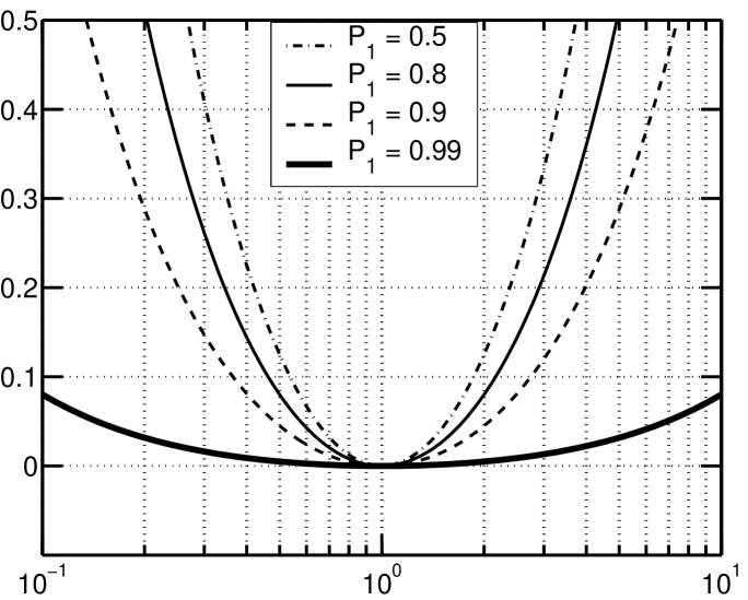
$\frac{k_{1}}{k_{2}}$

Figure 11: Difference series ($t=0,m=0$) $\Delta A_{0}(0)$ normalized by the solution in the fast-switching limit $\langle x^{2}\rangle_{\infty}$ as a function of the spring constant ratio, at various probabilities. (P₁ is the probability of being in state 1.) Note that when this ratio is 1 both statse are mechanically indistinguishable.

Satisfying these two conditions, the solution for the auto-correlation function deviates from the limiting forms on the order of 5% or greater. However, this does not guarantee applicability. The next condition that we impose regards limiting the number of terms in the series needed for adequately convergence to the desired solution. Here we are interested in cases for which the series solutions, Eqs. 54 and 55, are within the predefined tolerance (5% of $\bigl{\langle}x^{2}\bigr{\rangle}$) of the exact solution only after the calculation of three expansion terms. Figure 12 plots the $t=0$ difference series $\Delta A_{m}(0)$ (normalized by $\text{k}_{\text{\tiny B}}\text{T}$/$k_{a}$) for two different spring constant ratios at various probabilities, as a function of the number of expansions terms. We choose the spring constant ratio to be 2 in figure (a) and 3 in figure (b), recalling that it must be greater than 1.5 to be within our initial refined parameter list. From Fig. 12(a) it is evident that truncation of the series solution at second order is sufficient to allow for convergence to within 5% accuracy of the exact solution. From Fig. 12(b), however, it takes more terms. To be within the experimental tolerance of 5%, the series must contain at least four terms.

As stated in Sect. III (Eq. 56) there are no first order corrections; therefore, only one (three) expansion term (terms) are needed to be within this predefined error tolerance for these cases. For spring constants ratios greater than 3 more terms are needed. Therefore, this analysis gives an upper bound on our spring constant ratio to be less than 3.

The analysis presented in this section gives a range of parameters for which we believe this theory should be useful and practical for determining the rates of transition (for the two state problem) from experimental measurements, those which are not accessible from traditional means. To determine the rates of transition the solution for the auto-correlation function must deviate from both limiting forms, requiring the rate of transitions to be of the order of the inverse time constant of the experimental probe, $\{\kappa_{ij}\}\approx 1/\tau_{a},i\neq j$. To be within 5% accuracy of the exact solution and not near one of the limiting forms, the probability of being in either state should be greater than 10% and the ratio of the spring constants should also be greater than 1.5. To limit the number of calculated terms in the series to three or less, the ratio of the spring constants should also be less than 3.

(a)

$A_{m}(0)\bigl{\langle}k\bigr{\rangle}/\text{k}_{\text{\tiny B}}\text{T}$

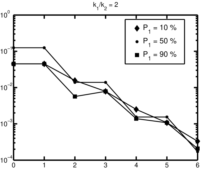
Number of Expansion Terms

(b)

$A_{m}(0)\bigl{\langle}k\bigr{\rangle}/\text{k}_{\text{\tiny B}}\text{T}$

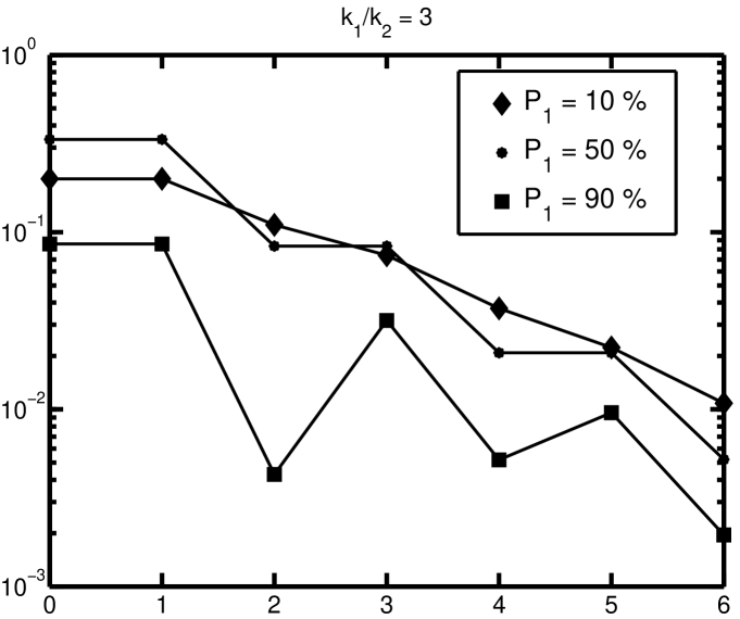
Number of Expansion Terms

Figure 12: Difference series $A_{m}(0)$ normalized by $\bigl{\langle}k\bigr{\rangle}/\text{k}_{\text{\tiny B}}\text{T}$ plotted as a function of the number of expansion terms, for $k_{1}/k_{2}=2$ (a) and $k_{1}/k_{2}=3$ (b), for various probabilities. P₁ is the probability of lying in state 1.

This range of parameters is somewhat limited; however, this method still provides an alternative to standard analysis, expanding the temporal capabilities alloted in experimental studies. Having obtained this range of parameters for applicability we now present calculated terms in both series, up to third order, for the two state Markov process. These solutions are amiable to experimental analysis, whose form depends on the value of the individual rates. Guided with our understanding of convergence obtained in this section, we then compare our truncated analytic series solutions to the numerical results presented in Sect. II.2.

V.1.2 Solutions for the Markov process

Our system of interest is a two state Markov process, a system consisting of two distinct mechanical states (different spring constants) whose transitions are local in time (independent of all previous configurations). Appendix D presents the detailed mathematics describing the two state Markov process and the solution for the auto-correlation function truncated at third order, Eqs. 91 and 93. Here we compare those solutions with the numerical solutions presented in Sect. II.2 and determine the degree of convergence.

Figure 13 redisplays the numerical solutions for case D presented in Sect. II.2. Recall, case D corresponds to a system where the rates of transition are of order of the inverse of the intrinsic time constant of the experimental probe (see Table 1). In addition, solutions corresponding to the fast-switching limit (solid blue line) and slow-switching limit (solid red line), see Fig. 8, are also redisplayed. To make connections with the previous analysis regarding convergence, the ratio of the spring constants for the two states is 1.8 ($k_{1}=45$pN/$\mu$m, $k_{2}=25$pN/$\mu$m) and the probability of lying in state 1 is 30%. These conditions nearly satisfy those displayed in Fig. 12 (a) and close to the limit we imposed for applicability. From Fig. 12 (a) we expect the convergence of both series to be within 1% of the exact solution. The analytic solutions truncated at third order are also displayed in the figure. The series expressed around the fast-switching limit, Eq. 91, is represented by the red dashed-line and the series expressed around the slow-switching limit, Eq. 93, is represented by the blue dashed-line. As expected, both series truncated at third order accurately portrays the numerical solution for case D.

Figure 13: Auto-correlation function for a system with a fluctuating spring constant. Numerical solutions for case D is represented by the red circles. The solid red line is the solution in the fast-switching limit and the blue line is the solution in the slow switching limit. Series solutions for the auto-correlation function, truncated at third order, are represented by the red dashed-line when initiated from the fast-switching limit solution (Eq. 91) and by the blue dashed-line when initiated from the slow-switching limit solution (Eq. 93).

The molecular parameters expressed in case D are near the region of minimal acceptable spatial resolution. Spatial resolution was enhanced when the spring constant associated with state 1 was increased to $k_{1}=140$pN/$\mu$m, which we termed as case $\mathcal{D}$. This results in a spring constant ratio of $k_{1}/k_{2}=5.6$, which is somewhat outside the predicted bounds for applicability. To test this idea, Fig. 14 presents the numerical solutions for case $\mathcal{D}$ along with the truncated series solutions. The numerical solutions are again represented by red circles, the solutions in the fast-switching limit is represented by the solid blue line and slow-switching limit is represented by the solid red line. The analytic solution expressed around the fast-switching limit, Eq. 91, is represented by the red dashed-line and the analytic solution expressed around the slow-switching limit, Eq. 93, is represented by the blue dashed-line. As expected, both series truncated at third order do not accurately portrays the numerical solution for case $\mathcal{D}$.

Figure 14: Auto-correlation function for a system with a fluctuating spring constant. Numerical solutions for case $\mathcal{D}$ is represented by the red circles. The solid red line is the solution in the fast-switching limit and the blue line is the solution in the slow switching limit. Series solutions for the auto-correlation function, truncated at third order, are represented by the red dashed-line when initiated from the fast-switching limit solution (Eq. 91) and by the blue dashed-line when initiated from the slow-switching limit solution (Eq. 93).

VI Conclusion

In this work we presented an analytic method applicable to the analysis of data from single-molecule switching experiments. This method regards the analysis of the auto-correlation. The auto-correlation function was taken as the vehicle for analysis, because it varies on time scales governed by the intrinsic time constant of the experimental probe and; therefore, its functional form should be effected by biomolecular transitions which occur on such corresponding time scales. This is an important attribute, because we presented arguments (theoretically motivated) to why this is also a temporal regime inaccessible for exploration by traditional averaging schemes; expanding the temporal capabilities of single molecule studies.

To bolster this position, we also presented mock (numerical simulations) experiments, demonstrating the failure of traditional averaging methods to predict both the mechanical and kinetic properties of biomolecular systems, when the transitions between the biomolecular states occur on the time scales governing the motion of the experimental probe. To further motivate the attributes of the auto-correlation function, we also presented numerical solutions which demonstrated how its functional form alters in this temporal regime. To comprehend how the auto-correlation function may be influenced by the rates of transition, we then presented two physically motivated guesses for its solution. We argued that these two guesses should correspond to solutions for the auto-correlation function in two physically opposing extremes: when the switching between biomolecular states is either much faster or much slower than the time scales governing the motion of the probe.

Motivated by these numerical simulations we then presented our mathematical analysis for the solution to the auto-correlation function. We modeled the experimental probe as an over-damped particle, in which the associated spring constants corresponding to the biomolecule fluctuates between different states. We presented a formal solution for the auto-correlation function, from which we proved that the two physically motivated solutions also correspond to mathematical bounds (opposing) to the general solution.

Although no known “closed” form solution exists for the problem at hand, we presented series solutions for the auto-correlation function. Inspired by the bounds found for the general solution, two series solutions for the auto-correlation function were expressed around these bounds; providing series solutions which converge to the exact solutions from opposing positions. In addition, we proved mathematically that the two bounds indeed correspond to exact solutions for the auto-correlation function in the anticipated regimes.

Having obtained two series solutions for the auto-correlation function we next presented a general analysis regarding their convergence to the general solution and their applicability to the analysis of single-molecule switching experiments. To garner concrete understanding regarding the convergence and applicability of this method, we then focuses on the two state problem. A range of biomolecular parameters, for where we believe this method would be applicable for the analysis of experimental data, was then determined. Guided by this analysis, we then presented solutions for each series (up to third order) for a two state Markov process. We compared our truncated series solutions with numerical solutions for the auto-correlation function and showed that these truncated series solutions converged to the numerical solution to the degree anticipated from our general analysis regarding convergence. These truncated series solutions for the auto-correlation function are amiable to the analysis of experimental data, in the regime where traditional averaging procedures fail.

The general analysis presented here should be applicable to single-molecule experimental studies. Although the range of parameters found for applicability of this method appears to be limited, this parameter range is beyond the reach for analysis with current traditional methods, providing an expanded region of phase space that can be explored by single-molecule methods.

Appendix A Variance of A Time Averaged Property

We now present an argument determining the reduction of the width of the distribution function for time averaged values $\langle x\rangle_{\rm T}$. The widths of the distribution functions are related to the square root of the variance, $\sigma^{2}$. Consider measurements of a property $x$ over a given time window T and the average value of this measurement, $\langle x\rangle_{\rm T}$, is tabulated. The relationship between the data set corresponding to the time averaged value to that of the data set corresponding to the instantaneous measurements is characterized by the following equality

$$\left(\begin{array}[]{c}\bigl{\langle}x\bigr{\rangle}_{1}\\ \\ \bigl{\langle}x\bigr{\rangle}_{2}\\ \vdots\\ \bigl{\langle}x\bigr{\rangle}_{\rm N}\end{array}\right)=\frac{1}{\text{M}}\left(\begin{array}[]{c}\sum_{j=1}^{\rm M}x_{1,j}\\ \\ \sum_{j=1}^{\rm M}x_{2,j}\\ \vdots\\ \sum_{j=1}^{\rm M}x_{N,j}\end{array}\right).$$ (60)

Here $x_{i,j}$ corresponds to an instantaneous measurement of $x$ and the time averaged value $\langle x\rangle_{i}$ corresponds to the average of $x$ over time window $i$. Each time window corresponds to M data points and there are a total of N$\times$M instantaneous measurements.

Now we make a comparison between the variance corresponding to the instantaneous measurements (whole data set),

$$\sigma_{x}^{2}=\frac{1}{\rm NM}\sum_{i,j}^{\rm N,M}\bigl{(}x_{i,j}-\bar{x}\bigr{)}^{2},$$ (61)

with that of the time averaged value,

$$\sigma_{\langle x\rangle_{\rm T}}^{2}=\frac{1}{\rm N}\sum_{i}^{\rm N}\left(\bigl{\langle}x\bigr{\rangle}_{i}-\bar{x}\right)^{2}.$$ (62)

Here $\bar{x}$ is the average value of $x$,

$$\bar{x}=\frac{1}{NM}\sum_{i,j}^{\rm N,M}x_{i,j}.$$ (63)

A few assumptions are now made. First it is assumed that the instantaneous measurements are uncorrelated, statistically independent. This implies that the instantaneous measurements are stored at time intervals on order of the intrinsic time constant of the experimental probe, as this is roughly the time scale to make two uncorrelated measurements. Next, we assume that the size of the data set corresponding to the time averaged value (N) is “large” such this data set ($\{\bigl{\langle}x\bigr{\rangle}_{i}\}$) adequately samples the distribution space of the time averaged value. Furthermore, we assume that the number of data points used to compute each averaged value (M) is “small” such that the distribution function corresponding to the time averaged value contains a measurable width, $\sigma_{\langle x\rangle_{\rm T}}\neq 0$. (This also implies N$\gg$M.) Finally, we assume that all distribution functions have mirror symmetry around the mean ($\bar{x}$) of the measured value $x$. These conditions are consistent with many single molecule experiments.

Given these assumptions we are now in position to relate the variance corresponding to the instantaneous measurements, $\sigma^{2}_{x}$, to that corresponding to the time averaged measurements, $\sigma^{2}_{\langle x\rangle_{\rm T}}$. The variance corresponding to the time averaged value, as expressed in Eq. 62, can be related to the instantaneous measurements as follows,

$$\sigma_{\langle x\rangle_{\rm T}}^{2} = \frac{1}{\rm N}\sum_{i}^{\rm N}\left(\bigl{\langle}x\bigr{\rangle}_{i}-\bar{x}\right)^{2}$$ (64)

$$= \frac{1}{\rm N}\sum_{i}^{N}\left(\frac{1}{\rm M}\sum_{j}^{\rm M}x_{i,j}-\bar{x}\right)^{2}$$ (65)

$$= \frac{1}{\rm NM^{2}}\sum_{i}^{\rm N}\left(\sum_{j}^{\rm M}\bigl{(}x_{i,j}-\bar{x}\bigr{)}\right)^{2}.$$ (66)

Because of the assumption that M is small, implying that $\sum_{j}^{\rm M}x_{i,j}/M\neq\bar{x}$, the last term does not vanish. This is consistent with having a nonzero variance corresponding to the time averaged value, $\sigma_{\langle x\rangle_{\rm T}}\neq 0$.

Further decomposing, the variance (Eq. 66) can be written as

$$\sigma_{\langle x\rangle_{\rm T}}^{2} = \frac{1}{\rm NM^{2}}\sum_{i}^{\rm N}\sum_{j}^{\rm M}\bigl{(}x_{i,j}-\bar{x}\bigr{)}^{2}$$ (68)

$$+\frac{1}{\rm NM^{2}}\sum_{i}^{\rm N}\sum_{j\neq k}^{M,M}\bigl{(}x_{i,j}-\bar{x}\bigr{)}\bigl{(}x_{i,k}-\bar{x}\bigr{)}.$$

Next, we use the assumption that N is “large”. In the limit that N goes to infinity the last term in Eq. 68 vanishes,

$$\lim_{N\rightarrow\infty}\sum_{i}^{\rm N}\bigl{(}x_{i,j}-\bar{x}\bigr{)}\bigl{(}x_{i,k}-\bar{x}\bigr{)}=0,$$ (69)

for $j\neq k$. This equality holds when the data set $\bigl{\langle}x\bigr{\rangle}_{\rm T}$ contain a number of statistically independent points and the distribution function has mirror symmetry around the average value $\bar{x}$.

The variance corresponding to the time averaged value now can be written as

$$\sigma_{\langle x\rangle_{\rm T}}^{2} = \frac{1}{\rm NM^{2}}\sum_{i}^{\rm N}\sum_{j}^{\rm M}\bigl{(}x_{i,j}-\bar{x}\bigr{)}^{2}$$ (70)

$$= \frac{1}{\rm M}\left(\frac{1}{\rm NM}\sum_{i,j}^{\rm N,M}\bigl{(}x_{i,j}-\bar{x}\bigr{)}^{2}\right)$$ (71)

$$= \frac{1}{\rm M}\sigma^{2}_{x}.$$ (72)

Revealing that the variance corresponding to the time average value is equal to the variance corresponding to the instantaneous measurements, $x$, reduced by the number of uncorrelated measurements used to determine the time averaged value.

Appendix B Time constant

The time scales governing the motion of the probe correspond to its time constant $\tau=\gamma/k$, where $k$ is the spring constant associated with the end of the probe. This time scale is also the time scale at which two uncorrelated measurements are made. This spring constant contains contributions from both the intrinsic time constant of the experimental probe, $k_{\rm P}$, and that from the molecule in state $i$, $k_{{\rm m}i}$. This time constant is less than the intrinsic time constant of the experimental probe, $\tau_{\rm P}=\gamma/k_{\rm P}$. For systems of interest the spring constant of the probe is generally much larger than or of order of the molecule in any state and; therefore, the intrinsic time constant of the experimental probe serves as an appropriate measure for the relaxation time of the probe when attached to a biomolecule, $\tau_{\rm P}\approx\tau$. Using the intrinsic time constant of the probe as the measure of its relaxation also proves to be a convenient measure, as the particular state of the molecule does not have to be continually referred to and quantified during this analysis. (Certainly, the discussions here can be generalized to the cases when the spring constant of the molecule in any state is much larger than the intrinsic spring constant of the probe.)

Appendix C Auto-correlation function, when $\langle f(t_{1})f(t_{2})\cdots f(t_{n})\rangle$ is independent of time

If all of the moments of the random variable $f$ are independent of the time variables then Eq. 45 takes the form

$$\bigl{\langle}\delta x(t)\delta x(0)\bigr{\rangle}=$$ (73)

$$\frac{\text{k}_{\text{\tiny B}}\text{T}}{k_{a}}\sum_{n,n^{\prime}=0}^{\infty}\frac{C_{n+n^{\prime}}}{\tau_{d}^{n+n^{\prime}}}\int_{0}^{\infty}\prod_{i=0}^{n}dt_{i}\prod_{i^{\prime}=0}^{n^{\prime}}dt_{i^{\prime}}e^{-\frac{|t+T_{n}-T_{n^{\prime}}|+T_{n}+T_{n^{\prime}}}{\tau_{a}}},$$

where

$$C_{n+n^{\prime}}=\bigl{\langle}\mathcal{F}_{n}(0,\{T_{j}\})\mathcal{F}_{n^{\prime}}(t,\{T_{j^{\prime}}\})\bigr{\rangle}$$

is independent of the time variables. It, therefore, only depends on the sum of $n$ and $n^{\prime}$ and not their individual values.

To evaluate this integral we first calculate the Fourier transform of the auto-correlation function and then integrate over the time variables. We will then take the inverse transform by using the residue theorem for complex integration. Finally, through algebraic identities we obtain the result in Eq. 51.

The Fourier transform $\hat{f}(\omega)$ of a function $f(t)$ is defined as

$$\hat{f}(\omega) = \int_{-\infty}^{\infty}dtf(t)e^{-i\omega t}$$

and the inverse transform is defined as

$$f(t) = \frac{1}{2\pi}\int_{-\infty}^{\infty}d\omega\hat{f}(\omega)e^{i\omega t}.$$

The Fourier transform of the auto-correlation function in this limiting form is

$$\bigl{\langle}\hat{x}(\omega)x(0)\bigr{\rangle} = \frac{\text{k}_{\text{\tiny B}}\text{T}}{k_{a}}\sum_{n,n^{\prime}=0}^{\infty}\left(\frac{1}{\tau_{d}^{n+n^{\prime}}}\right)\frac{2C_{n+n^{\prime}}/\tau_{a}}{(1/\tau_{a})^{2}+\omega^{2}}$$

$$\times\int_{0}^{\infty}\prod_{i=0}^{n}dt_{i}e^{-t_{i}(\frac{1}{\tau_{a}}-i\omega)}\prod_{i^{\prime}=0}^{n^{\prime}}dt_{i^{\prime}}e^{-t_{i}^{\prime}(\frac{1}{\tau_{a}}+i\omega)}.$$

Integrating over all the time variables, $\{t_{i}\}$ and $\{t_{i^{\prime}}\}$, the Fourier transform becomes

$$\bigl{\langle}\hat{x}(\omega)x(0)\bigr{\rangle} = \frac{\text{k}_{\text{\tiny B}}\text{T}}{k_{a}}\sum_{n,n^{\prime}=0}^{\infty}\left(\frac{1}{\tau_{d}^{n+n^{\prime}}}\right)\frac{C_{n+n^{\prime}}}{\tau_{a}/2}$$

$$\times\left(\frac{i}{\omega+i/\tau_{a}}\right)^{n+1}\left(\frac{-i}{\omega-i/\tau_{a}}\right)^{n^{\prime}+1}.$$

Taking the inverse transform of Eq. C the auto-correlation function is

$$\bigl{\langle}\delta x(t)\delta x(0)\bigr{\rangle} = \frac{\text{k}_{\text{\tiny B}}\text{T}}{k_{a}}\sum_{n,n^{\prime}=0}^{\infty}\left(\frac{1}{\tau_{d}^{n+n^{\prime}}}\right)\frac{C_{n+n^{\prime}}}{\tau_{a}/2}\int_{-\infty}^{\infty}d\omega e^{i\omega t}$$

$$\times\frac{1}{2\pi}\left(\frac{i}{\omega+i/\tau_{a}}\right)^{n+1}\left(\frac{-i}{\omega-i/\tau_{a}}\right)^{n^{\prime}+1}$$

or

$$\bigl{\langle}\delta x(t)\delta x(0)\bigr{\rangle} = \frac{\text{k}_{\text{\tiny B}}\text{T}}{k_{a}}\sum_{n,n^{\prime}=0}^{\infty}\left(\frac{i}{\tau_{d}}\right)^{n+n^{\prime}}\frac{C_{n+n^{\prime}}}{\tau_{a}\pi}\left(\frac{\tau_{a}}{i^{3}}\right)^{n^{\prime}}\frac{1}{n^{\prime}!}$$ (75)

$$\left.\times\frac{\partial^{n^{\prime}}}{\partial a^{n^{\prime}}}\int_{-\infty}^{\infty}d\omega e^{i\omega t}\frac{\left(\omega+i/\tau_{a}\right)^{-n-1}}{\omega-ia/\tau_{a}}\right|_{a=1}.$$

Equation 75 can be integrate in the upper-half complex-plane. The integrand has a pole at $\omega=ia/\tau_{a}$ and

$$\bigl{\langle}\delta x(t)\delta x(0)\bigr{\rangle} = \frac{\text{k}_{\text{\tiny B}}\text{T}}{k_{a}}\sum_{n,n^{\prime}=0}^{\infty}2\left(\frac{\tau_{a}}{\tau_{d}}\right)^{n+n^{\prime}}C_{n+n^{\prime}}\frac{(-1)^{n^{\prime}}}{n^{\prime}!}$$ (76)

$$\left.\times\frac{\partial^{n^{\prime}}}{\partial a^{n^{\prime}}}\frac{e^{-at/\tau_{a}}}{(1+a)^{n+1}}\right|_{a=1}.$$

Using the identity

$$\frac{\partial^{n^{\prime}}}{\partial a^{n^{\prime}}}AB=\sum_{j=0}^{n^{\prime}}\frac{n^{\prime}!}{j!(n^{\prime}-j)!}A^{[j]}B^{[n^{\prime}-j]},$$

where $X^{[j]}$ is the $j^{th}$ derivative of $X$, and switching variables to $m=n+n^{\prime}$ and $n^{\prime}$, Eq. 76 can be written as

$$\bigl{\langle}\delta x(t)\delta x(0)\bigr{\rangle} = \frac{\text{k}_{\text{\tiny B}}\text{T}}{k_{a}}e^{-t/\tau_{a}}\sum_{m=0}^{\infty}\left(\frac{\tau_{a}}{\tau_{d}}\right)^{m}C_{m}$$

$$\times\sum_{n^{\prime}=0}^{m}\sum_{j=0}^{n^{\prime}}\frac{(m-j)!}{j!(n^{\prime}-j)!(m-n^{\prime})!}\left(\frac{t}{\tau_{a}}\right)^{j}\frac{1}{2^{m-j}}.$$

Using the identity

$$\sum_{n^{\prime}=0}^{m}\sum_{j=0}^{n^{\prime}}=\sum_{j=0}^{m}\sum_{n^{\prime}=j}^{m}$$

Equation C can be written as

$$\bigl{\langle}\delta x(t)\delta x(0)\bigr{\rangle} = \frac{\text{k}_{\text{\tiny B}}\text{T}}{k_{a}}e^{-t/\tau_{a}}\sum_{m=0}^{\infty}\left(\frac{\tau_{a}}{\tau_{d}}\right)^{m}C_{m}\sum_{j=0}^{m}\left(\frac{t}{\tau_{a}}\right)^{j}\frac{1}{2^{m-j}}\frac{(m-j)!}{j!}\sum_{n^{\prime}=j}^{m}\frac{1}{(n^{\prime}-j)!(m-n^{\prime})!}$$ (78)

$$= \frac{\text{k}_{\text{\tiny B}}\text{T}}{k_{a}}e^{-t/\tau_{a}}\sum_{m=0}^{\infty}\left(\frac{\tau_{a}}{\tau_{d}}\right)^{m}C_{m}\sum_{j=0}^{m}\left(\frac{t}{\tau_{a}}\right)^{j}\frac{1}{2^{m-j}}\frac{(m-j)!}{j!}\sum_{l=0}^{m-j}\frac{1}{(m-j-l)!l!}$$

$$= \frac{\text{k}_{\text{\tiny B}}\text{T}}{k_{a}}e^{-t/\tau_{a}}\sum_{m=0}^{\infty}\left(\frac{\tau_{a}}{\tau_{d}}\right)^{m}C_{m}\sum_{j=0}^{m}\frac{1}{j!}\left(\frac{t}{\tau_{a}}\right)^{j},$$

the desired result.

Appendix D Expansion for a two state Markov process

We present solutions for the series expansions represented in Eqs. 54 and 55, up to third order, for a system that behaves as a two state Markov process. Here, a biomolecule is considered a two state Markov process if two distinct mechanical states exist (different spring constants) and the probability of making a transition from one state to another is local in time (independent of all previous configurations). We provide closed form solutions for the auto-correlation function (truncated at third order) that depends on the magnitude of the rates and can be used in the analysis of experimental data. We proceed by first reviewing the relevant theory of a two state Markov process.

D.1 The two state problem: Statistics

We review some statistics governing a two state Markov process. Particularly, properties required for the evaluation of the moments ($\mathcal{D}^{(\infty)}_{n,n^{\prime}},\mathcal{D}^{(0)}_{n,n^{\prime}}$) expressed in the solution of the auto-correlation function, Eqs. 54 and 55.

Consider a two state Markov process and assume that at time $t=0$ the system starts in state $i$ . The probability of the system lying in state $j$ at time t obeys the following rate equation

$$\frac{\partial}{\partial t}\left(\begin{array}[]{l}P_{i1}(t)\\ P_{i2}(t)\end{array}\right)=\left(\begin{array}[]{rr}-\kappa_{12}&\kappa_{21}\\ \kappa_{12}&-\kappa_{21}\end{array}\right)\left(\begin{array}[]{l}P_{i1}(t)\\ P_{i2}(t)\end{array}\right).$$ (79)

Here $P_{ij}(t)$ is the probability of the system lying in state $j$ at time $t$ if at time $t=0$ the system was in state $i$, $\kappa_{21}$ is the rate of going into state 1 from state 2 and $\kappa_{12}$ is the rate of going into state 2 from state 1.

Define the rate matrix as

$$\mathbf{W}\equiv\left(\begin{array}[]{rr}-\kappa_{12}&\kappa_{21}\\ \kappa_{12}&-\kappa_{21}\end{array}\right).$$

The probability of the system lying in a particular state ($P_{ij}$) at time $t$ follows from solving the differential equation represented in Eq. 79. In matrix notation the solution is

$$\vec{P}(t)=\mathbf{T}_{t}\vec{P}(0),$$ (80)

Here the transition probability matrix, $\mathbf{T}_{t}$, is defined as

$$\mathbf{T}_{t}\equiv e^{\mathbf{W}t},$$ (81)

whose ($i,j$) component, $T_{t,ij}$, is defined as the probability of the system lying in state $i$ at time $t$ if it was in state $j$ at time 0. Because we assume a Markov process, the stationary solution to Eq. 80 and the transition probability matrix is all that is needed to obtain the statistics governing the transitions of the system. All higher order, multi-variable, joint probability distributions functions can be obtained from them.

The stationary solution to Eq. 80 is

$$\vec{P}=\left(\begin{array}[]{c}P_{1}\\ P_{2}\end{array}\right),$$ (82)

where

$$P_{1} = \kappa_{21}/\kappa,$$

$$P_{2} = \kappa_{12}/\kappa$$

and

$$\kappa=\kappa_{21}+\kappa_{12}.$$ (83)

It is straightforward to show that the transition probability matrix is

$$\mathbf{T}_{t}=\mathbf{1}-(1-e^{-\kappa t})\left(\begin{array}[]{rr}P_{2}&-P_{1}\\ -P_{2}&P_{1}\end{array}\right),$$

where $\mathbf{1}$ is the identity matrix.

For the moment we refine our discussion to instances of time. The stochastic variable of interest is the fluctuating term $f(t)$, Eq. 36. At time $t_{n}$ the value of the fluctuating term is denoted as $f^{(n)}$, which can take one of two values: $f_{1}$ if in state 1 and $f_{2}$ if in state 2. For the problem at hand these values are $f_{i}=\mp 1$, where the minus sign corresponds to the system with the larger spring constant, (see Eq. 36). Because we now consider instances of time we define slight variants to the stationary probability solution, $\vec{P}$, and transition probability matrix, $\mathbf{T}_{t}$. These variants refer to particular values of $f$ instead of particular states of the system. The stationary probability of $f$ having value $f^{(n)}$ is denoted as $\mathbb{P}_{1}(f^{(n)})$ (single variable probability distribution function) . The probability of $f$ having value $f^{(\alpha)}$ at time $t_{\alpha}$ if it have had value $f^{(\beta)}$ at time $t_{\beta}$ is denoted as $T_{t_{\alpha,\beta}}(f^{(\alpha)}|f^{(\beta)})$.

The multi-variable joint probability distribution functions, defined as the probability of $f$ having value $f^{(n)}$ at time $t_{n}$ if $f$ had value $f^{(n-1)}$ at time $t_{n-1}$ and value $f^{(n-2)}$ at time $t_{n-2}$ and so on, is

$$\mathbb{P}_{n}(f^{(1)},t_{1};f^{(2)},t_{2};\cdots;f^{(n)},t_{n})=$$

$$T_{t_{n,n-1}}(f^{(n)}|f^{(n-1)})\cdots T_{t_{3,2}}(f^{(3)}|f^{(2)})T_{t_{2,1}}(f^{(2)}|f^{(1)})$$

$$\times\mathbb{P}_{1}(f^{(1)}).$$

Here time is ordered, $t_{1}\leq t_{2}\leq....\leq t_{n}$, and $t_{m,m-1}\equiv t_{m}-t_{m-1}\geq 0$ is the time difference of neighboring time instances.

Averages over the stochastic variable $f$ are needed to evaluate the integrals in Eqs. 54 and 55. They can be written as

$$\bigl{\langle}f(t_{1})f(t_{2})...f(t_{n})\bigr{\rangle}=$$

$$\sum_{f^{(1)}\cdots f^{(n)}=\{f_{1},f_{2}\}}f^{(1)}f^{(2)}\cdots f^{(n)}\mathbb{P}_{n}(f^{(1)},t_{1};\cdots;f^{(n)},t_{n})$$

or in an alternative matrix form

$$\bigl{\langle}f(t_{1})f(t_{2})...f(t_{n})\bigr{\rangle}=\bigl{(}f_{1}\ \ f_{2}\bigr{)}\biggl{(}\prod_{i=1}^{n-1}\bigl{(}\mathbf{T}_{1}+e^{-\kappa t_{i,i-1}}\mathbf{T}_{2}\bigr{)}\biggr{)}\vec{P},$$ (84)

where $t_{1}\leq t_{2}\leq...\leq t_{n}$ (time ordering). Here

$$\mathbf{T}_{1} = \left(\begin{array}[]{cc}f_{1}P_{1}&f_{2}P_{1}\\ f_{1}P_{2}&f_{2}P_{2}\end{array}\right),$$ (87)

$$\mathbf{T}_{2} = \left(\begin{array}[]{cc}f_{1}P_{2}&-f_{2}P_{1}\\ -f_{1}P_{2}&f_{2}P_{1}\end{array}\right).$$ (90)

Given the averages of the fluctuating term, Eq. 84, terms in the series expansion can be evaluated for the general case.

D.2 Truncated series

Using the definitions above, we calculated the general solution for the auto-correlation, up to third order. Expanding around the fast-switching limit the auto-correlation function takes the form

$$\bigl{\langle}x(t)x(0)\bigr{\rangle}_{3}^{(\infty)}=\frac{\text{k}_{\text{\tiny B}}\text{T}}{\bigl{\langle}k\bigr{\rangle}}e^{-t\langle\tau^{-1}\rangle}+\frac{\text{k}_{\text{\tiny B}}\text{T}}{k_{a}}\left(\frac{\tau_{a}}{\tau_{d}}\right)^{2}4P_{1}P_{2}e^{-t/\tau_{a}}\left[\left(\vec{C}_{2}+e^{-\kappa t}\vec{D}_{2}\right)^{\dagger}\vec{T}_{2}(t)+\frac{\tau_{a}}{\tau_{d}}\bigl{\langle}f\bigr{\rangle}\left(\vec{C}_{3}+e^{-\kappa t}\vec{D}_{3}\right)^{\dagger}\vec{T}_{3}(t)\right],$$ (91)

where the superscript ($(\infty)$) denotes that the series is expanded around the fast-switching limit and the subscript denotes the order at which the series is truncated. In Eq. 91 we present new notation. The vector $\vec{T}_{n}(t)$ is a $n$-component vector that is a function of time and defined as

$$\vec{T}_{n}(t)=\left(\begin{array}[]{c}1\\ \frac{t}{\tau_{a}}\\ \vdots\\ \frac{1}{(n-1)!}\left(\frac{t}{\tau_{a}}\right)^{(n-1)}\end{array}\right).$$ (92)

The coefficient vectors, $\vec{C}_{n}$ and $\vec{D}_{n}$, are functions of $\kappa\tau_{a}$, whose values are listed in Table 2. Dagger ($\dagger$) represents the transpose of a vector and $\bigl{\langle}f\bigr{\rangle}=f_{1}P_{1}+f_{2}P_{2}$ is the average value of the fluctuating variable. The subscripts on the vectors $\vec{T}_{n}(t),\ \vec{C}_{n}$ and $\vec{D}_{n}$ represents the order each term was calculated, second or third, and also corresponds to the size of the vector. In limit that $\kappa\tau_{a}\rightarrow\infty$ the coefficient vectors in Eq. 91 vanish, leaving only the fast-switching limit solution.

As expressed in Sect. V, once the fast-switching limit is determined expansion around the slow-switching limit is easily determined by exploiting Eqs. 91 and V:

$$\bigl{\langle}x(t)x(0)\bigr{\rangle}_{3}^{(0)}=\left\langle\frac{\text{k}_{\text{\tiny B}}\text{T}}{k}e^{-t/\tau}\right\rangle+\frac{\text{k}_{\text{\tiny B}}\text{T}}{k_{a}}\left(\frac{\tau_{a}}{\tau_{d}}\right)^{2}4P_{1}P_{2}e^{-t/\tau_{a}}\left[\left(\vec{C}_{2}+e^{-\kappa t}\vec{D}_{2}-1\right)^{\dagger}\vec{T}_{2}(t)+\frac{\tau_{a}}{\tau_{d}}\bigl{\langle}f\bigr{\rangle}\left(\vec{C}_{3}+e^{-\kappa t}\vec{D}_{3}-1\right)^{\dagger}\vec{T}_{3}(t)\right],$$ (93)

where the superscript ($(0)$) denotes that the series is expanded around the slow-switching limit. Here, in the limit that $\kappa\tau_{a}\rightarrow 0$ the terms in the square brackets sum to zero, leaving the slow-switching limit solution.

Table 2: Coefficients for two state Markov process in the fast-switching limit. The indices for the vectors $\vec{C}$ and $\vec{D}$ are denoted by the subscripts. The coefficients for the slow-switching limit is determined trivial through these coefficients and the use of Eq. V.

Coefficients	Value ($\alpha=\kappa\tau_{a}$)
$C_{2,1}$	$\frac{2\alpha^{2}+\alpha-2}{(2+\alpha)\alpha^{2}}$
$C_{2,2}$	$\frac{1}{\alpha}$
$D_{2,1}$	$\frac{2-\alpha}{(2+\alpha)\alpha^{2}}$
$D_{2,2}$	0
$C_{3,1}$	$\frac{(17/4)\alpha^{4}+(11/2)\alpha^{3}-4\alpha^{2}+4\alpha+16}{(2+\alpha)^{2}\alpha^{3}}$
$C_{3,2}$	$\frac{(7/2)\alpha^{2}-6}{(2+\alpha)\alpha^{2}}$
$C_{3,3}$	$\frac{2}{\alpha}$
$D_{3,1}$	$\frac{-\alpha^{3}+4\alpha^{2}-4\alpha-16}{(2+\alpha)^{2}\alpha^{3}}$
$D_{3,2}$	$\frac{\alpha-2}{(2+\alpha)\alpha^{2}}$
$D_{3,3}$	0

Equations 91 and 93 are general solutions for the auto-correlation function. These solutions depend on the magnitude of the rates of transition for the molecule, $\kappa_{12}$ and $\kappa_{21}$, unlike the solutions in the fast-switching and slow-switching limits, which depend only on the ratio of the rates.

References

- Finzi and Gelles (1995) L. Finzi and J. Gelles, Science 267, 378 (1995).
- Smith et al. (1996) S. B. Smith, Y. Cui, and C. Bustamante, Science 271, 795 (1996).
- Mehta et al. (1997) A. D. Mehta, J. T. Finer, and J. A. Spudich, Proc. Natl. Acad. Sci. USA 94, 7927 (1997).
- Rief et al. (1997a) M. Rief, F. Oesterhelt, B. Heymann, and H. E. Gaub, Science 275, 1295 (1997a).
- Rief et al. (1997b) M. Rief, M. Gautel, F. Oesterhelt, J. M. Fernandez, and H. E. Gaub, Science 276, 1109 (1997b).
- Guilford et al. (1997) W. H. Guilford, D. E. Dupuis, G. K. ans J. Wu, J. B. Patlak, and D. M. Warshaw, Biophys. J. 72, 1006 (1997).
- Oberhauser et al. (1998) A. F. Oberhauser, P. E. Marszalek, H. P. Erickson, and J. M. Fernandez, Nature 393, 181 (1998).
- Veigel et al. (1998) C. Veigel, M. L. Bartoo, D. C. S. White, J. C. Sparrow, and J. E. Molloy, Biophys. J. 75, 1424 (1998).
- Carrion-Vazquez et al. (1999) M. Carrion-Vazquez, P. E. Marszalek, A. F. Oberhauser, and J. M. Fernandez, Proc. Natl. Acad. Sci. USA 96, 11288 (1999).
- Marszalek et al. (1999) P. E. Marszalek, H. Lu, H. Li, M. Carrion-Vazquez, A. F. Oberhauser, K. Schulten, and J. M. Fernandez, Nature 402, 100 (1999).
- Rief et al. (1999) M. Rief, J. Pascual, M. Saraste, and H. E. Gaub, J. Mol. Biol. 286, 553 (1999).
- Veigel et al. (1999) C. Veigel, L. M. Coluccio, J. D. Jontes, J. C. Sparrow, R. A. Milligan, and J. E. Molloy, Nature 398, 530 (1999).
- Meiners and Quake (2000) J. C. Meiners and S. R. Quake, Phys. Rev. Lett 84, 5014 (2000).
- Oberhauser et al. (2001) A. F. Oberhauser, P. K. Hansma, M. Carrion-Vazquez, and J. M. Fernandez, Proc. Natl. Acad. Sci. USA 98, 468 (2001).
- Liphardt et al. (2001) J. Liphardt, B. Onoa, S. B. Smith, I. T. Jr., and C. Bustamante, Science 292, 733 (2001).
- Marszalek et al. (2002) P. E. Marszalek, H. Li, A. F. Oberhauser, and J. M. Fernandez, Proc. Natl. Acad. Sci. USA 99, 4278 (2002).
- Schwaiger et al. (2002) I. Schwaiger, C. Sattler, D. R. Hostetter, and M. Rief, Nature Materials 1, 232 (2002).
- Baker et al. (2002) J. E. Baker, C. Brosseau, P. E. Joel, and D. M. Warshaw, Biophys. J. 82, 2134 (2002).
- Lia et al. (2003) G. Lia, D. Bensimon, V. Croquette, J.-F. Allemand, D. Dunlap, D. E. A. Lewis, S. Adhya, and L. Finzi, Proc. Natl. Acad. Sci. USA 100, 11373 (2003).
- Jacob et al. (1999) M. Jacob, G. Holtermann, D. Perl, J. Reinstein, T. Schindler, M. A. Geeves, and F. X. Schmid, Biochemistry 38, 2882 (1999).
- Mayor et al. (2000) U. Mayor, C. M. Johnson, V. Daggett, and A. R. Fersht, Proc. Natl. Acad. Sci. USA 97, 13518 (2000).
- Crane et al. (2000) J. C. Crane, E. K. Koepf, J. W. Kelly, and M. Gruebele, J. Mol. Biol. 298, 283 (2000).
- Myers and Oas (2002) J. K. Myers and T. G. Oas, Annu. Rec. Biochem. and referenced there in. 71, 783 (2002).
- Hughes and Wang (2003) W. L. Hughes and Z. L. Wang, Appl. Phys. Lett. 82, 2886 (2003).
- Bargatin et al. (2005) I. Bargatin, E. D. Myers, J. Arlett, B. Gudlewski, and M. L. Roukes, Appl. Phys. Lett. 86, 133109 (2005).
- Hatfield and Quake (1999) J. W. Hatfield and S. R. Quake, Phys. Rev. Lett 82, 3548 (1999).
- Patlak (1993) J. B. Patlak, Biophys. J. 65, 29 (1993).
- van Gunsteren and Berendsen (1982) W. F. van Gunsteren and H. J. C. Berendsen, Mol. Phys. 45, 637 (1982).
- Bourret et al. (1973) R. Bourret, U. Frisch, and A. Pouquet, Physica A 65, 303 (1973).
- Brissaud and Frisch (1974) A. Brissaud and U. Frisch, J. Math. Phys. 15, 524 (1974).
- van Kampen (1975) N. G. van Kampen, Phys. Rep. p. 172 (1975).
- Roerdink (1981) J. B. T. M. Roerdink, Physica A 109, 23 (1981).
- Lindenberg et al. (1981) K. Lindenberg, V. Seshadri, and B. J. West, Physica A 105, 445 (1981).
- Roerdink (1982) J. B. T. M. Roerdink, Physica A 112, 557 (1982).
- Ikeda (2000) N. Ikeda, J. Phys. A 33, 6385 (2000).
- Gradshteyn and Ryzhik (1994) I. S. Gradshteyn and I. M. Ryzhik, Table of Integrals, Series, and Products (Academic Press, 1994), 5th ed.